Lane Changing
- Compatibility
Requirements Engineering
Requirements Engineering
- The process of defining, documenting, and maintaining requirements
- 6 steps:
- Requirements inception (需求獲取)
- Requirements analysis(需求分析)
- Requirements specification(需求規格)
- Requirements validation(需求驗證)
- Requirements management(需求管理)
Requirements Engineering in our case
- Original requirements: collision-free
- Issue: incompatible between systems
- Requirements inception
- compatibility
- Requirements analysis, specification, validation
- (research objective)
- guarantee compatibility under some conditions ?
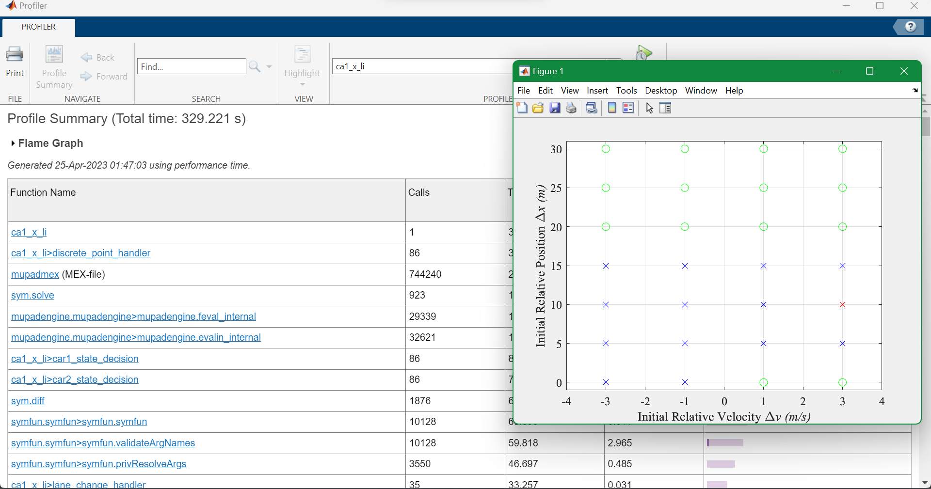
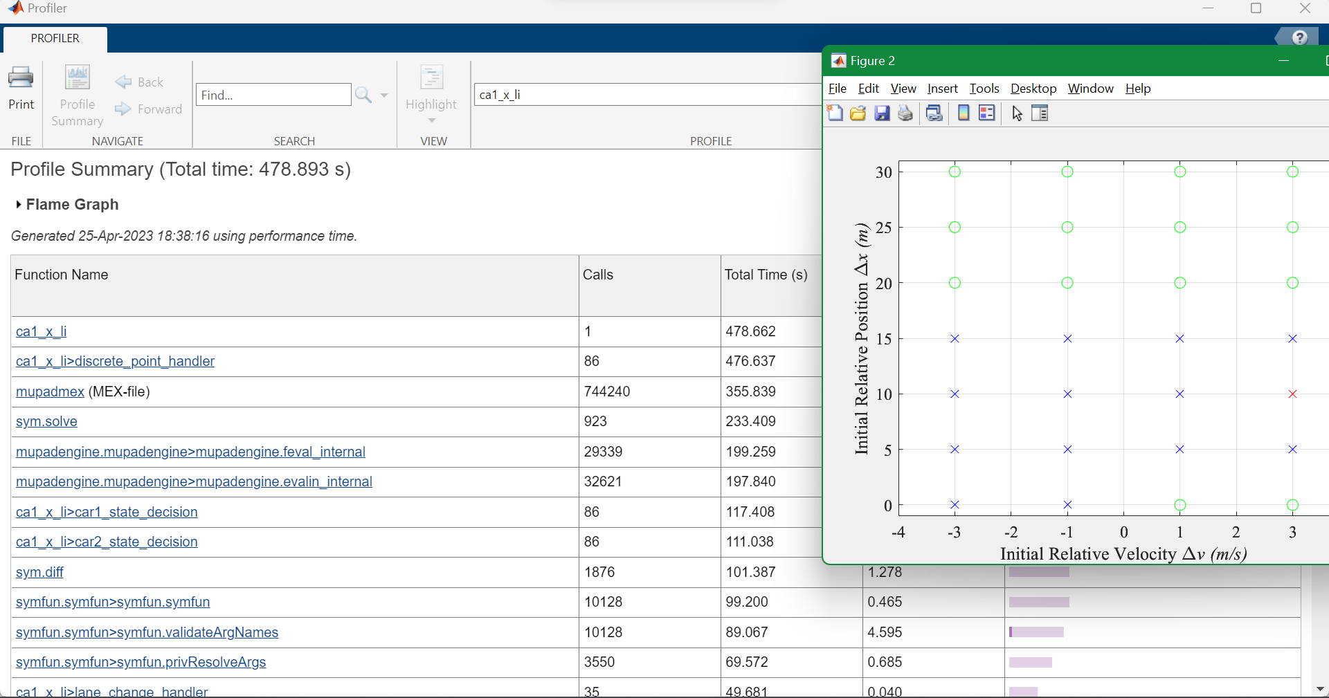
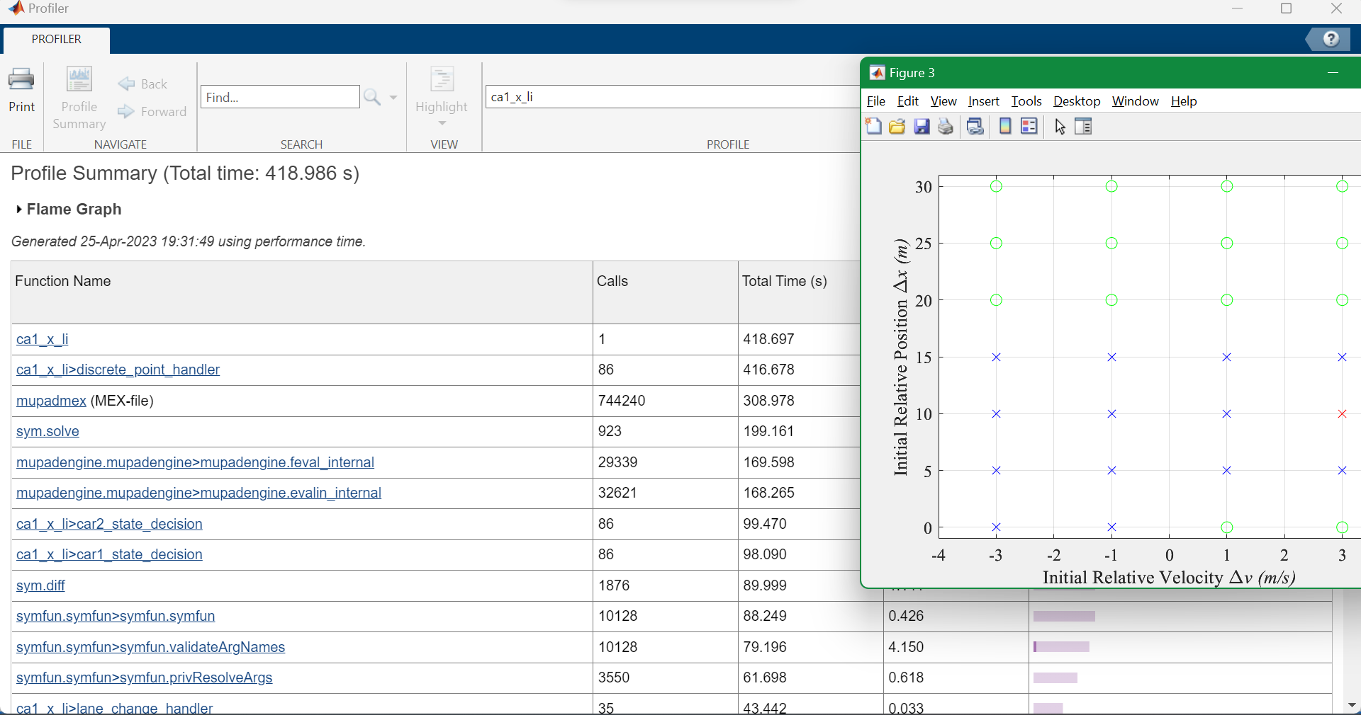
Speed-up: 15% / 20%~30%
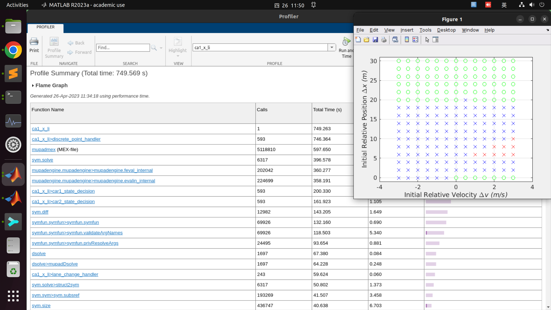
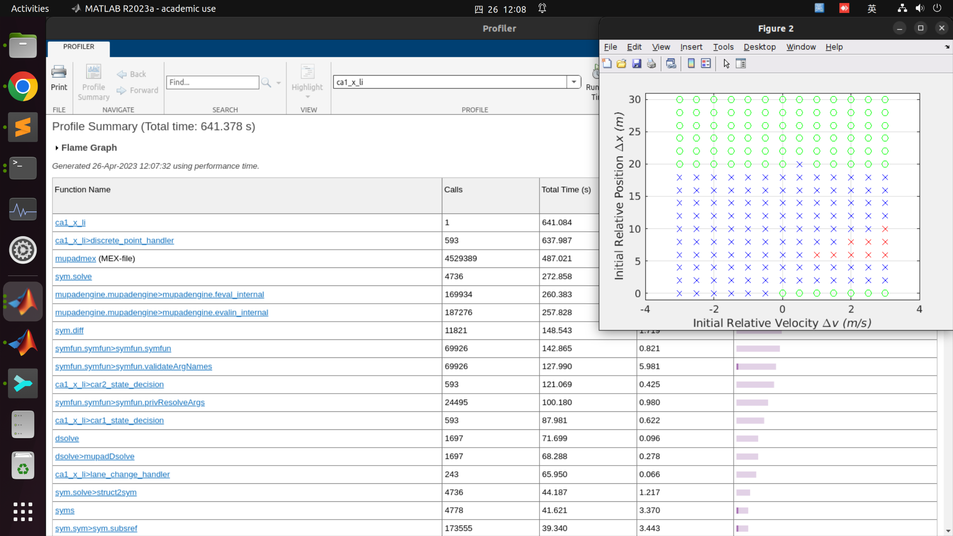
Speed-up: 15% / 20%~30%
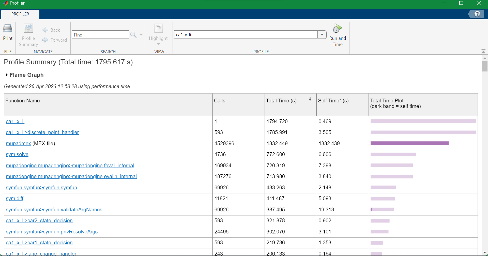
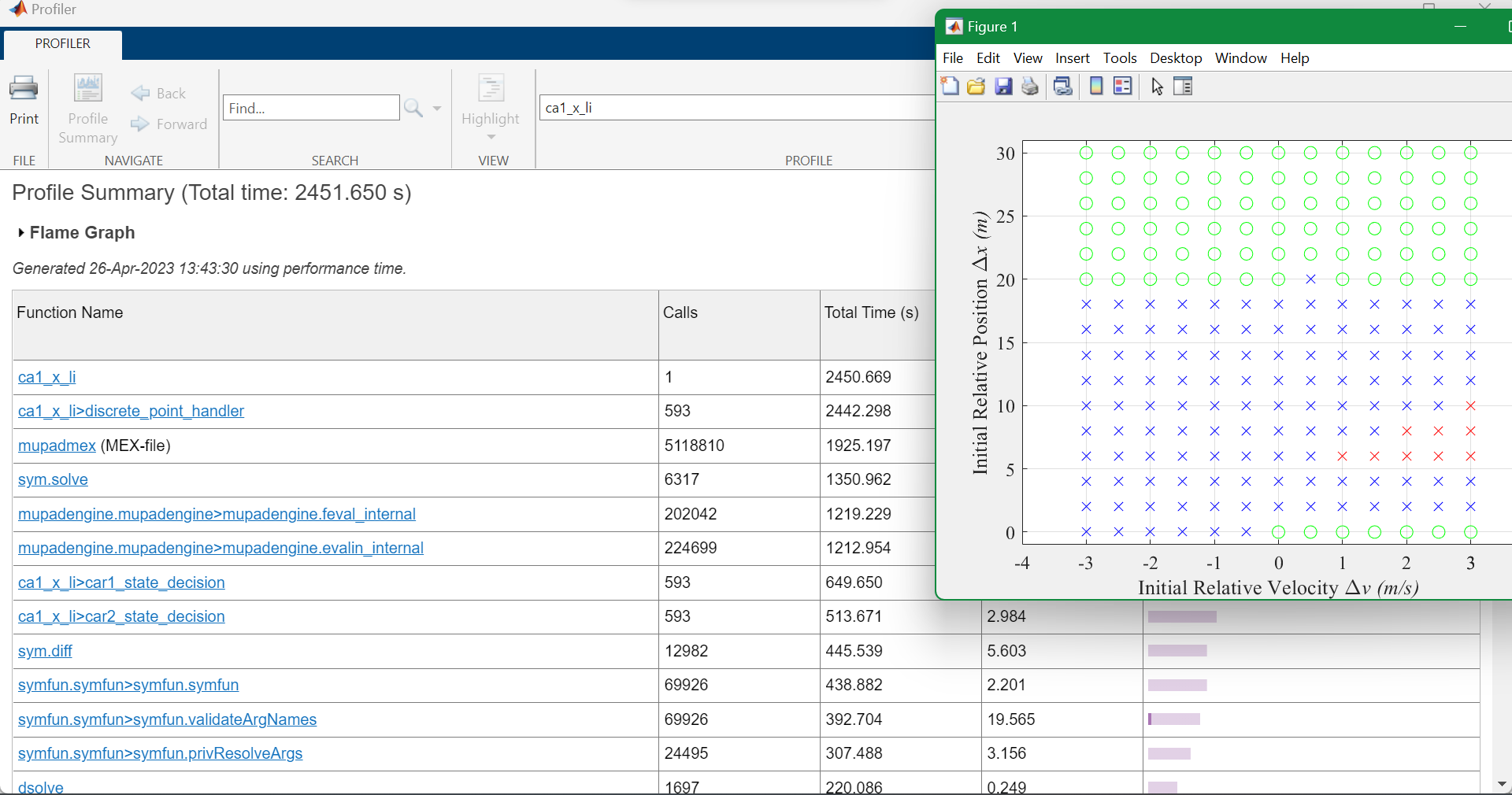
Speed-up: 15% / 20%~30%
ca1
加速
等速
減速
\(v = v_{\min}\)
\(v = v_{\max}\)
\(x' - x = d_{\min}\)
\(\neg blue \land \neg red\)
\(\neg blue\)
\(x' - x = d_{\min}\)
變換車道(\(|x - x'| > d_{lc}\))
ca1
加速
等速
減速
\(v = v_{\min}\)
\(v = v_{\max}\)
\(x < x' \land x' - x < d_{\min}\)
\(\neg blue \land \neg red\)
\(\neg blue\)
\(x < x' \land x' - x < d_{\min}\)
變換車道(\(|x - x'| > d_{lc}\))
li
線性加速
等加速
等減速
等速max
等速min
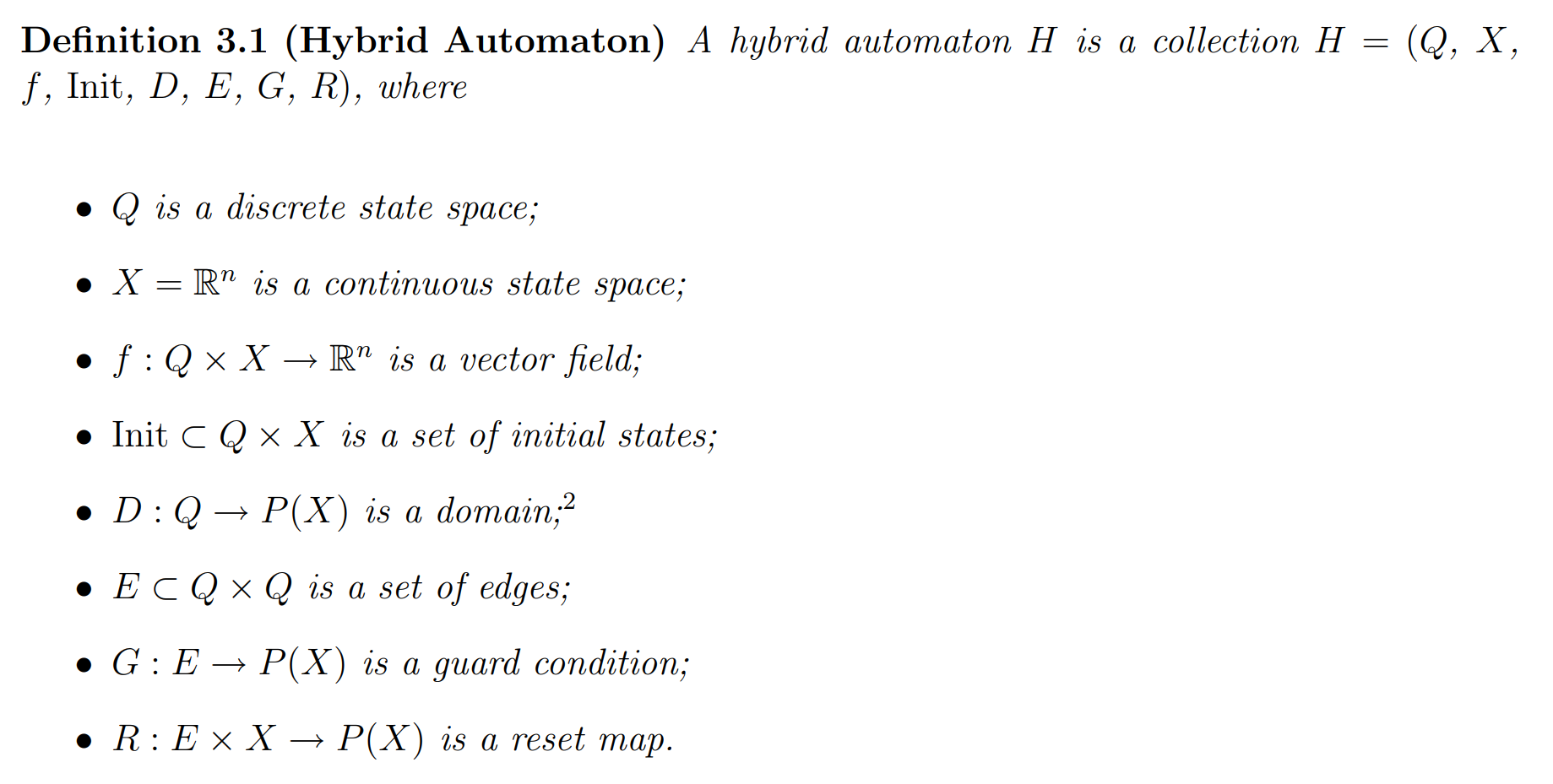

\(q_1\in Q\)
\(q_2\in Q\)
continuous state: \(X = \mathbb{R}^n, f\)

\(\dfrac{dx}{dt} = f_{q_1}(x)\)
constraints
\(x\in D(q_1)\)
\(x\in D(q_2)\)
\(x\in G(q_1, q_2)\)
\(e \in E\)
\(\dfrac{dx}{dt} = f_{q_2}(x)\)
\(x \gets R(e, x)\)
discrete state/graph: \(Q, E\)
constraints: \(D_{omain}, G_{uard}\)
def PeriodicSimulation(
    Q, #                  discrete state space
    X, # = R^n            continuous state space
    f, # = Q × X → R^n    vector field
    Init, # = Q × X       set of initial states
    D, # Q → P(X)         domain
    E, # in Q × Q         set of edges
    G, # E → P(X)         guard condition
    R, # E × X → P(X)     reset map
):
    dt = 0.000001
    q, x = pick(Init)
    while True:
        # edge case
        if x not in D(q):
            raise Exception("OUT_OF_DOMAIN")
        # change state (discrete transition)
        next = []
        for q2 in Q:
            if ((q, q2) in E) and (x in G(q, q2)) and (x in D(q2)):
                next.append(q2)
        # same state (continuous evolution)
        x2 = x + f(q, x) * dt
        if x2 in D(q):
            next.append(STAY)
        # test blocked
        if is_empty(next):
            raise Exception("BLOCKED")
        # choose nondeterministically
        q2 = pick(next)
        if q2 == STAY:
            x = x2
        else:
            x = pick(R((q, q2), x))
            q = q2
Issues
- Blocking / Non-blocking
- hard to verify
- Non-deterministic
- hard to verify
- Composability
- all variables are states
- Zeno execution?
- intentional deviation?
Simulation - Water Tank System
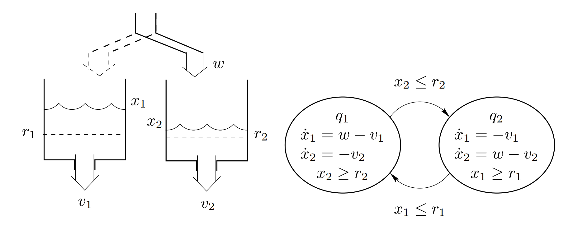
\(q_1\)
\(q_2\)
\(q_2\)
\(q_1\)
current
STAY
change state
\(dt\)
solution: binary search for the boundary
(discrete transition)
(continuous evolution)
import numpy as np
import random

def arr(*x): return np.array(x)
def pick(x): return random.choice(x)
def is_empty(x): return not bool(x)
def water(x, b = 1, l = 30, mx = 15):
    n = int(x / mx * l)
    s = '.' * n + ' ' * (l - n)
    b = int(b / mx * l)
    return s[:b] + '|' + s[b:]
DT = 0.001
eps = 1e-30
converge_threshold = 100

STAY = -1
def PeriodicSimulation(
    Q, #                  discrete state space
    X, # = R^n            continuous state space
    f, # = Q × X → R^n    vector field
    Init, # = Q × X       set of initial states
    D, # Q → P(X)         domain
    E, # in Q × Q         set of edges
    G, # E → P(X)         guard condition
    R, # E × X → P(X)     reset map
):
    q, x = pick(Init)
    t = 0
    convergence = (None, 0)
    while True:
        dt = DT
        while dt > eps:
            if not D(q, x):
                raise Exception("OUT_OF_DOMAIN")

            next = []
            for q2 in Q:
                if ((q, q2) in E) and (G(q, q2, x)) and (D(q2, x)):
                    next.append(q2)

            x2 = x + f(q, x) * dt
            if D(q, x2):
                next.append(STAY)

            if is_empty(next):
                dt /= 2
                continue

            q2 = pick(next)
            if q2 == STAY:
                x = x2
                t += dt
            else:
                x = R((q, q2), x)
                q = q2

            if convergence[0] == x.tolist():
                convergence = (convergence[0], convergence[1] + 1)
            else:
                convergence = (x.tolist(), 1)
            # print(convergence)
            if convergence[1] > converge_threshold:
                raise Exception("CONVERGED")
            break

        if not (dt > eps):
            raise Exception("BLOCKED")

        print(f'{q = },\t{water(x[0])},\t{water(x[1])},\t{t = },\tln(dt) = {int(np.log(dt))}')
        # print(f'{q = },\t{x = },\t{t = },\t{dt = }')

w = 0.5
v0 = 0.2
v1 = 0.4
r0 = 1
r1 = 1

np.set_printoptions(precision=3)
PeriodicSimulation(
    Q = [0, 1],
    X = None,
    f = lambda q, x: [arr(w-v0, -v1), arr(-v0, w-v1)][q],
    Init = [(0, arr(7, 7))],
    D = lambda q, x: [x[1] >= r1, x[0] >= r0][q],
    E = [(0, 1), (1, 0)],
    G = lambda q1, q2, x: { (0, 1): x[1] <= r1, (1, 0): x[0] <= r0 }[(q1, q2)],
    R = lambda qs, x: x,
)
Ca1
\(f_A(x, v) = (v, a)\)
\(Q = \{\ A = \text{加速},\ C = \text{等速},\ D = \text{減速}\ \}\)
\(f_C(x, v) = (v, 0)\)
\(f_D(x, v) = (v, -a)\)
\(R(\cdot, x) = x\)
\(D(A) = \{V \leq v_{\max}\}\)
\(G(\cdot, \cdot) = ?\)
\(D(D) = \{V \geq v_{\min}\}\)
ca0
\(L_{ane\ change}\)
\(A_{ccelerate}\)
\(C_{onstant\ speed}\)
\(D_{eccelerate}\)
high
low
\(D_L\)
\(D_A\)
\(D_D\)
\(D_C\)
priority
Flow
\((x_1', v_1') = (0, 0)\)
\((x_1', v_1') = (v_1, a_{\max})\)
\((x_1', v_1') = (v_1, a_{\min})\)
\((x_1', v_1') = (v_1, 0)\)
\(D_L \coloneqq |x_1 - x_2| \geq d_{\min}\)
\(D_A \coloneqq \begin{cases}v_2 < v_{\max} - v_\text{mgn}, &\text{ if }x_1 > x_2\\ v_2 < v_{\min} + v_\text{mgn}, &\text{ else}\end{cases}\)
\(D_C \coloneqq (v_1 = v_{\min}) \lor (v_1 = v_{\max})\)
\(D_D \coloneqq \begin{cases}v_2 > v_{\max} - v_\text{mgn}, &\text{ if }x_1 > x_2\\ v_2 > v_{\min} + v_\text{mgn}, &\text{ else}\end{cases} \coloneqq \neg D_A\)
ca0
high
low
priority
\(D_L \coloneqq |x_1 - x_2| \geq d_{\min} \coloneqq \begin{cases}x_1 - x_2 \geq d_{\min}, &\text{if }x_1 > x_2\\ x_2 - x_1 \geq d_{\min}, &\text{else}\end{cases}\)
\(D_A \coloneqq \begin{cases}(v_1 < v_{\max}) \land (v_2 < v_{\max} - v_\text{mgn}), &\text{if }x_1 > x_2\\ (v_1 < v_{\max}) \land (v_2 < v_{\min} + v_\text{mgn}), &\text{else}\end{cases}\)
\(D_C \coloneqq (v_{\min} \leq v_1) \land (v_1 \leq v_{\max})\)
\(D_D \coloneqq \begin{cases}(v_1 > v_{\min}) \land (v_2 > v_{\max} - v_\text{mgn}), &\text{ if }x_1 > x_2\\ (v_1 > v_{\min}) \land (v_2 > v_{\min} + v_\text{mgn}), &\text{ else}\end{cases}\)
\(D_L\)
\(D_A\)
\(D_D\)
\(D_C\)
\((x_1', v_1') = (0, 0)\)
\((x_1', v_1') = (v_1, a_{\max})\)
\((x_1', v_1') = (v_1, a_{\min})\)
\((x_1', v_1') = (v_1, 0)\)
\(L_{ane\ change}\)
\(A_{ccelerate}\)
\(C_{onstant\ speed}\)
\(D_{eccelerate}\)
\(v_{\min}=5,\;v_{\max}=25,\;v_{\text{mgn}}=3,\;d_{\min}=5,\;a_{\max}=3,\;a_{\min}=-2\)
Re-implementation
Model

Model

\(q_1\in Q\)
\(q_2\in Q\)
continuous state: \(X = \mathbb{R}^n, f\)


\(\dfrac{dx}{dt} = f_{q_1}(x)\)
constraints
\(x\in D(q_1)\)
\(x\in D(q_2)\)
\(x\in G(q_1, q_2)\)
\(e \in E\)
\(\dfrac{dx}{dt} = f_{q_2}(x)\)
\(x \gets R(e, x)\)
discrete state/graph: \(Q, E\)
constraints: \(D_{omain}, G_{uard}\)
Original Method
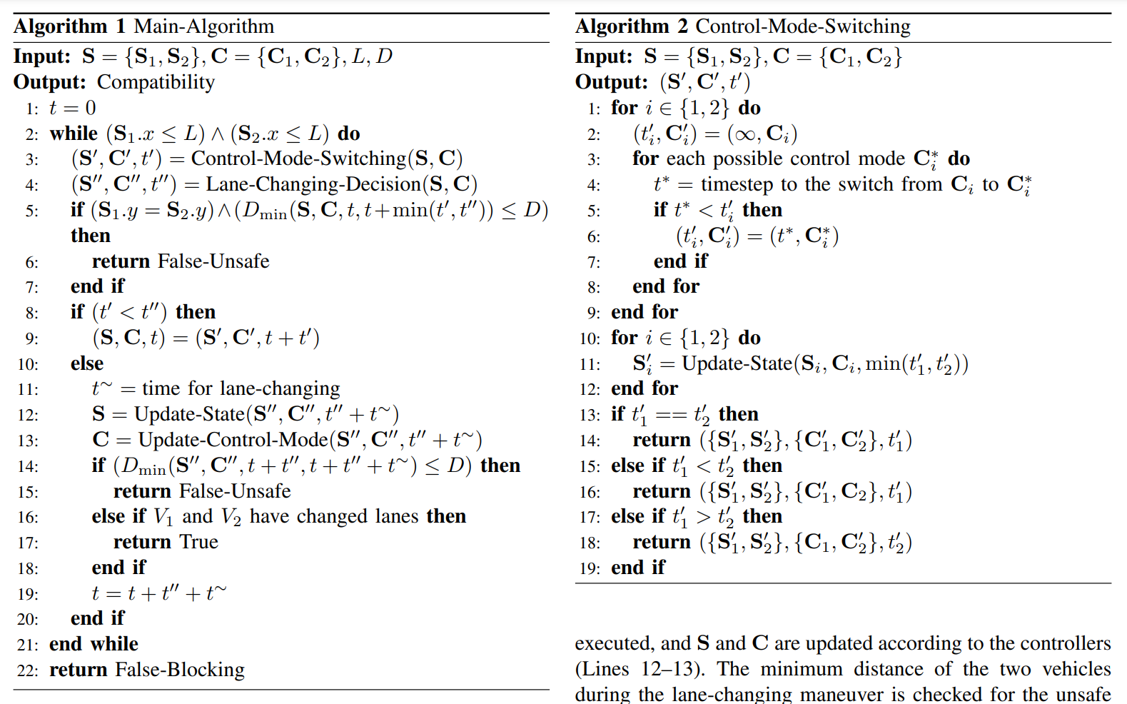
Bottleneck
Input: state \(q, x_0\); next state \(q'\)
Output: minimum \(\tau\) for transition \((q, x(\tau)) \rightarrow q'\)
\(\iff \min \tau: \begin{cases}x(0) &= x_0\\ x'(t) &= f_q(x(t))\\ x(\tau) &\in G_{q\rightarrow q'} \cap D_{q'} \end{cases}\)
\(\begin{cases}x(0) &= x_0\\ x'(t) &= f_q(x(t))\\ x(\tau) &\in G_{q\rightarrow q'} \cap D_{q'} \end{cases}\)
from sympy import symbols, Eq, Function, dsolve

X_0 = (10, 5)
A = 2
def f(x, v):
    return (v, A)

t = symbols("t")
X = symbols("X:2", cls=Function)
X = [x(t) for x in X]

equations = [
    Eq(x.diff(t), fx)
for x, fx in zip(X, f(*X))]

sol = dsolve(equations, X, ics={
    x.subs(t, 1e-30): x_0
for (x, x_0) in zip(X, X_0) })
print(sol)

min(sympy.solve(...).as_set().boundry) ?
\(\begin{cases}x(0) &= x_0\\ x'(t) &= f_q(x(t))\\ x(\tau) &\in G_{q\rightarrow q'} \cap D_{q'} \end{cases}\)
Cond = Cond & Cond
     = Cond | Cond
     = !Cond
     = f(X) >= 0
     (f is continuous)
Constraints on \(G\) and \(D\)
min(sympy.solve(...).as_set().boundry) ?
\(X \in G \iff \)Cond is true
Cond = Cond & Cond
     = Cond | Cond
     = !Cond
     = f(X) >= 0
     (f is continuous)


Decelerate = 車速 > v_min
           = !(v_min - v1 >= 0)

Accelerate = 車速 < v_max & (行駛於前 | 前車距離 > d_min)
           = !(v1 - v_max >= 0) & (x1 - x2 >= 0 | !(d_min - (x2 - x1) >= 0))
\(X \in G_{q\rightarrow q'} \cap D_{q'} \iff (f(X)\geq0 \lor g(X)\geq0)\land (\neg (h(X)\geq0))\)
\(\land\)
\(\lor\)
\(\neg\)
\(h(X) \geq 0\)
\(g(X) \geq 0\)
\(f(X) \geq 0\)
\(f\geq0\)
\(g\geq0\)
\(h\geq0\)
\(t\)
\(f\geq0\)
\(g\geq0\)
\(h\geq0\)
\(t\)
F
\(X \in G_{q\rightarrow q'} \cap D_{q'} \iff (f(X)\geq0 \lor g(X)\geq0)\land (\neg (h(X)\geq0))\)
\(f\geq0\)
\(g\geq0\)
\(h\geq0\)
\(t\)
F
\(X \in G_{q\rightarrow q'} \cap D_{q'} \iff (f(X)\geq0 \lor g(X)\geq0)\land (\neg (h(X)\geq0))\)
\(f\geq0\)
\(g\geq0\)
\(h\geq0\)
\(t\)
T
\(X \in G_{q\rightarrow q'} \cap D_{q'} \iff (f(X)\geq0 \lor g(X)\geq0)\land (\neg (h(X)\geq0))\)
Assumptions
- Solving for minimum positive root is easy
- \((f(X_t)\geq0 \lor g(X_t)\geq0)\land (\neg (h(X_t)\geq0))\)
- vs \(f(X_t) = 0\)
-
Condis general enough
Cond = Cond & Cond
     = Cond | Cond
     = !Cond
     = f(X) >= 0
     (f is continuous)
========REQUIREMENT===================
Root(F=>T)
========BASE CASES====================
Condition: f(x) > 0
T = min(nsolve(sols + f(x), [t] + X, [0] + X0))
F=>T = f(X0) > 0 ? inf : T
T=>F = f(X0) > 0 ? T : inf
========RECURSIVE CASES===============
Boolean: !A
F=>T = A(T=>F)
T=>F = A(F=>T)
Boolean: A&B
F=>T = (F&F,F&T,T&F)=>(T&T)
?= max(A(F=>T), B(F=>T))
T=>F = (T&T)=>(F&F,F&T,T&F)
= min(A(T=>F), B(T=>F))
Boolean: A|B
F=>T = (F|F)=>(T|T,F|T,T|F)
= min(A(F=>T), B(F=>T))
T=>F = (T|T,F|T,T|F)=>(F|F)
?= max(A(T=>F), B(T=>F))Tree DP optimization?
\(\land\)
\(\lor\)
\(\neg\)
\(h(X) \geq 0\)
\(g(X) \geq 0\)
\(f(X) \geq 0\)
a ? b : c
= (a & b) | ((!a) & c)
Graph optimization
\(\lor\)
\(\land\)
\(\land\)
\(a\)
\(b\)
\(b\)
\(a\)
\(b\)
\(c\)
\(\neg\)
a ? b : c
= (a & b) | ((!a) & c)
Graph optimization
\(\lor\)
\(\land\)
\(\land\)
\(a\)
\(b\)
\(b\)
\(a\)
\(b\)
\(c\)
\(\neg\)
Graph optimization
\(f_1(X) \geq 0\)
\(f_2(X) \geq 0\)
\(f_3(X) \geq 0\)
\(f_4(X) \geq 0\)
\(f_5(X) \geq 0\)
\(Cond_1\)
\(Cond_2\)
\(Cond_3\)
\(Cond_4\)
push the timeline synchronously
- Original:
- \(f(X) \geq 0 \implies\) T
- \(f(X) < 0 \implies\) F
- Improved:
- \(|f(X)| \leq \epsilon \implies\) X
- \(f(X) > \epsilon \implies\) T
- \(f(X) < \epsilon \implies\) F
Simulation improvement
- Accelerates to \(25\) m/s (max speed)
- \(v = 25.0000000001\) m/s
- \(D_C = \neg \text{too\_fast} \land \neg \text{too\_slow}\)
- Can't maintain constant speed
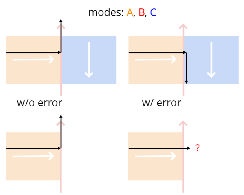
round-off error
round-off error
modes: A, B, C
w/o error
w/ error
?
Solutions
- Enforce boundary:
- Whenever blocked, move back to boundary
- Model check:
- Verify if behavior is defined on or across boundaries
- Verify if behavior is defined on or across boundaries
?
Robustness and Implementability of Timed Automata
Simplification
- Domain \(D = \top\)
- Guard \(G = \bigwedge (a_i \leq x_i \leq b_i)\) (linear & independent)
- Flow \(f(X) = (1, 1, \dots, 1)\) (clock)
Error Formulation
- drift on clocks \(\epsilon\)
- \((S_1, X_1) \overset{t \text{ secs}}{\longrightarrow} (S_2, X_2)\) \(\Rightarrow\) \((S_1, X_1) \overset{t(1-\epsilon) \sim t(1+\epsilon)}{\longrightarrow} (S_2, X_2)\)
- imprecision on guards \(\Delta\)
- \(a_i \leq x_i \leq b_i\) \(\Rightarrow\) \(a_i - \Delta \leq x_i \leq b_i + \Delta\)
mode A
mode B
mode C
mode D
- 偏差率 (\(\frac{Err}{\Delta t}\))
- \(f_A(X) \cdot \nabla G_{A \rightarrow B}\)
Lane Changing - Compatibility
short summary
Phase 1
-
Work on Existing Method
Phase 2
-
Redesign Model
Phase 3
-
Identify Difficulties
Work on Existing Method

Work on Existing Method
Achievement
- Speed up MATLAB code
Identified Issues
- No formal definition of lane-changing systems
- Imprecise implementation
- Hard to maintain the original code
Redesign Model


Redesign Model
Achievement
- Model hybrid systems based on this paper
- Add restrictions for Guard / Domain conditions
- Re-implement our paper's algorithm
- Complete discrete/continuous simulation
- Build visualization tools
Cond = Cond & Cond
     = Cond | Cond
     = !Cond
     = f(X) >= 0
     (f is continuous)
Identify Difficulties
- Limited power of equation solvers
- Unavoidable floating point errors
- Errors are expected in real world interactions
Possible Solution 1
Set-based verification
- Flow*
- Plenty of existing work
- No convenient tools yet
- Explosive states?
- May still work in most cases (trivial cases)
Possible Solution 2
Confidence score
Provide confidence score (robustness) about the simulated trace
- May assist in downstream task decisions
- Can't guarantee safety
Possible Solution 3
Restrictions on lane-changing systems
- How to determine restrictions?
- Linear boundaries?
- The models in some papers seem oversimplified
Another way to measure robustness?
(against real world errors)
Robustness + Falsification
Idea
Error => multiple possible traces
=> sample different traces
Assumptions
- \(\tau = \Delta t\) between two steps
- \(\tau\) follows uniform distribution between 0 and \(\epsilon\) (e.g. 0.001)
- deterministic hybrid system
init
\(\epsilon\)
\(\epsilon\)
\(\epsilon\)
\(\epsilon\)
\(\epsilon\)
init
minimum
robustness
\(\epsilon\)
\(\epsilon\)
\(\epsilon\)
\(\epsilon\)
\(\epsilon\)
init
minimum
robustness
sample break points
\(\epsilon\)
\(\epsilon\)
\(\epsilon\)
\(\epsilon\)
\(\epsilon\)
minimum
robustness
control
mode
control
mode
\(0.4\epsilon\)
\(p = 0.6\)
\(p = 0.4\)
Add-ons
- must sample between every control mode change
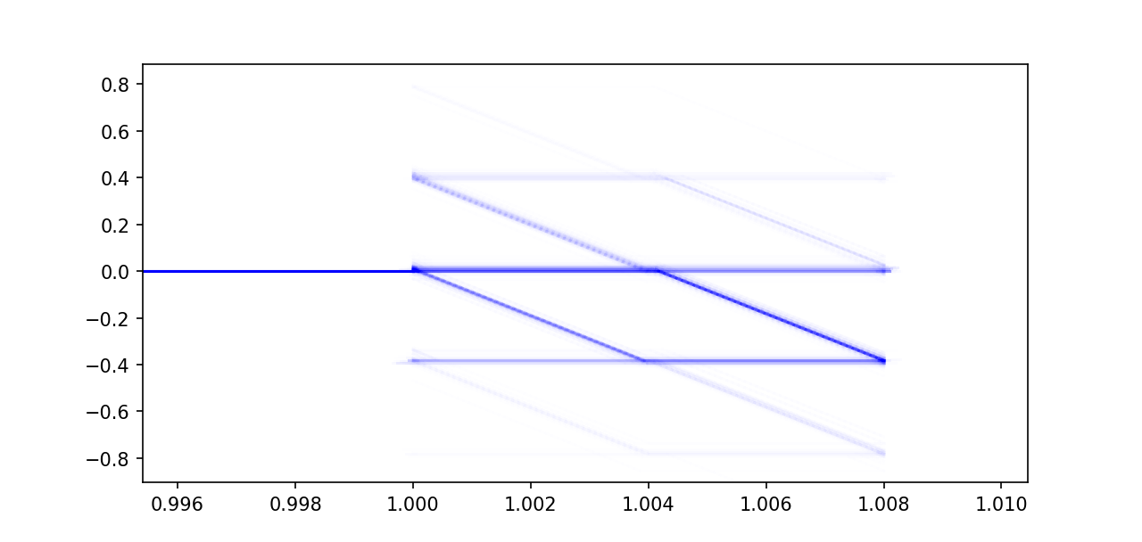
1 step
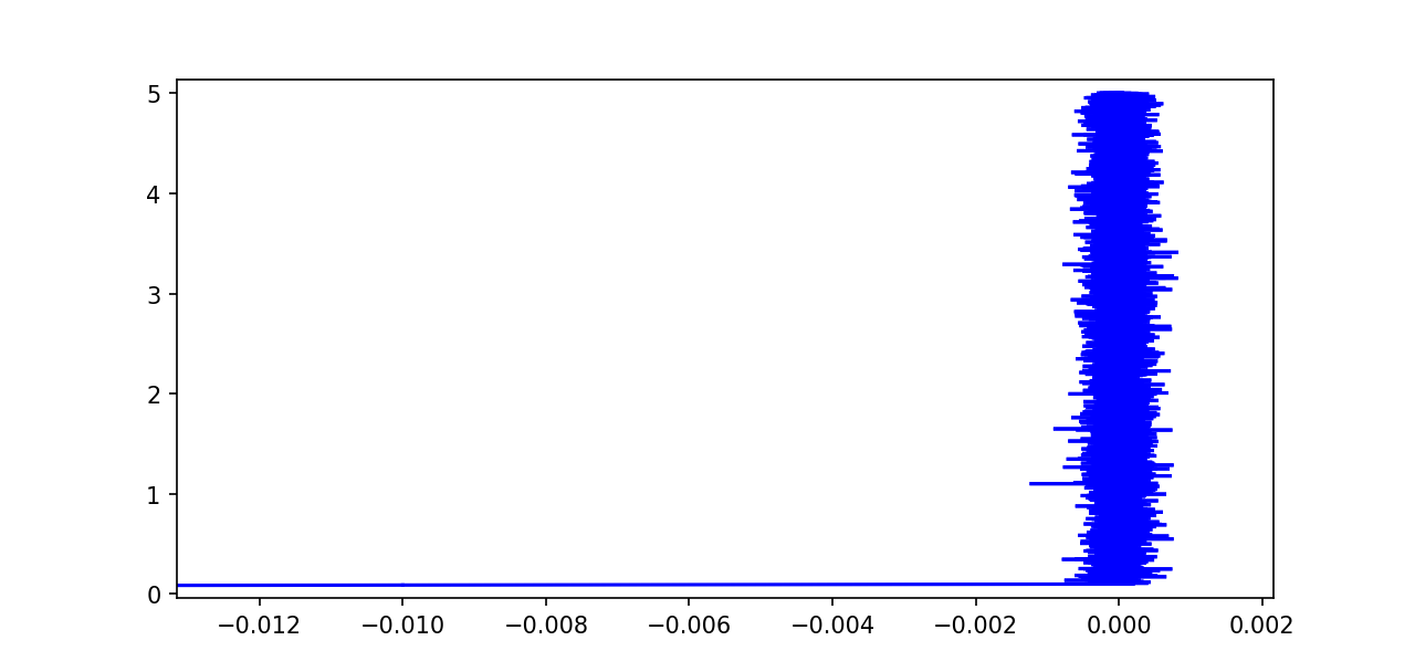
1 step
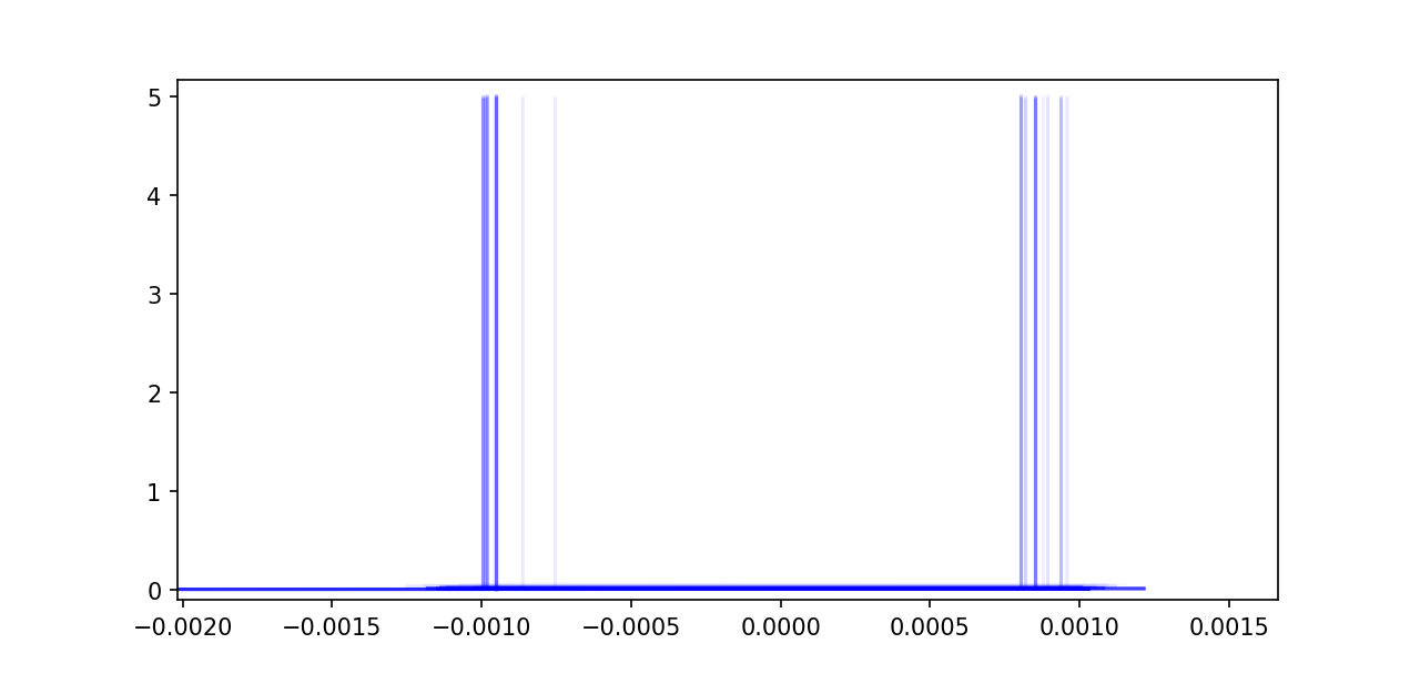
0.2 step
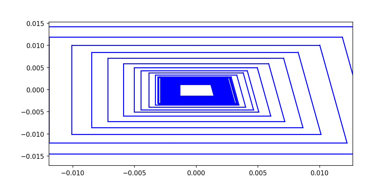
1 step
A
B
C
D
A
B
C
D
E
F
A
B
C
D
E
F
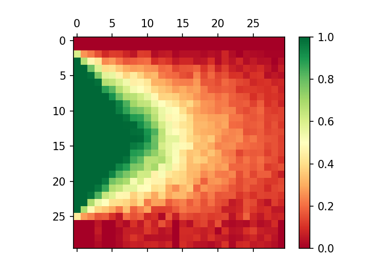
v
y
A
B
C
D
E
F

Robustness Improvement
TODO:
- some small bugs
- binary search for boundary (after sampling)
- use dijkstra in robustness improvement
- optimize for control mode oscillation
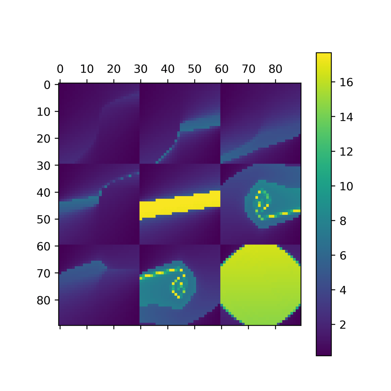
Ca0
Ca1
Agg
Ca0
Ca1
Agg
sample
\(\tau\)
\(t\)
\(\tau\)
p=0.5
p=0.25
p=0.25
1.
2.
3.
\(\tau\)
\(t\)
1.
2.
3.
low \(R\)
high \(R\)
high \(R\)
sample
4.
p=0.25
p=0.75
A
B
C
D
E
F
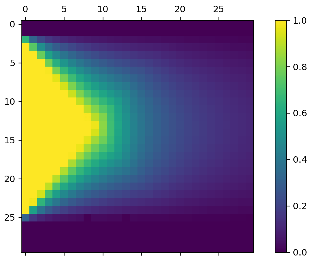
\(y\)
\(\tau\)
lane changing - compatibility
By thomaswang2003
lane changing - compatibility
- 541


