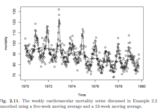
Example 2.2: Pollution, Temperature and Mortality
- study by Shumway (1988) - possible effects of temperature and pollution on weekly mortality
- strong seasonal components -> corresponds to summer-winter variation and downward trend in cardiovascular mortality over 10 years
- scatterplot matrix shows four models, Mt = cardiovascular mortality, Tt denotes temperature and Pt denotes the particulate levels
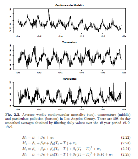
- As shown by the formulas, we can add in different factors such as linear temperature, curvilinear temperature, and pollution.
- Each model is a "better" model - accounting for some 60% of the variability and the best value of AIC and BIC (maximum likelihood)
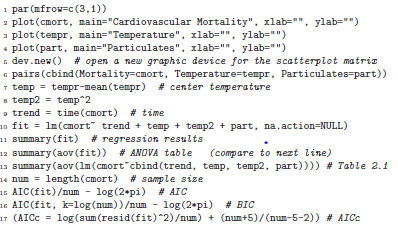
- the code for plotting and adding AIC/BIC:
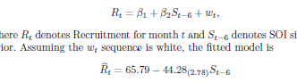
Regression w/ Lagged Variables
- If the time is measured at t -6 months instead of t months. The relationship might not be as linear as we thought.
Use ts.intersect to align the lagged series
Exploratory Data Analysis
- it is necessary for time series data to be stationary so its easy to average lagged products over time
- dependence between the values of the series is important to measure- at least be able to estimate auto-correlation with precision
- However, what if the series isn't stationary?
Use the mode: - xt = ut + yt where xt = observations, ut = trend and yt = stationary process
- we can subtract ut from both sides to establish a reasonable estimate for yt.
Example 2.4: Detrending Global Temperature
- Assume the model is in the form of the equation from 2.3. And also a classic straight line is our reasonable model
- Using ordinary least squares, we found the estimate for the trend line:
yt = xt + 11.2 - 0.006t - Shows ACF of the original data as well as the ACF of the detrended data
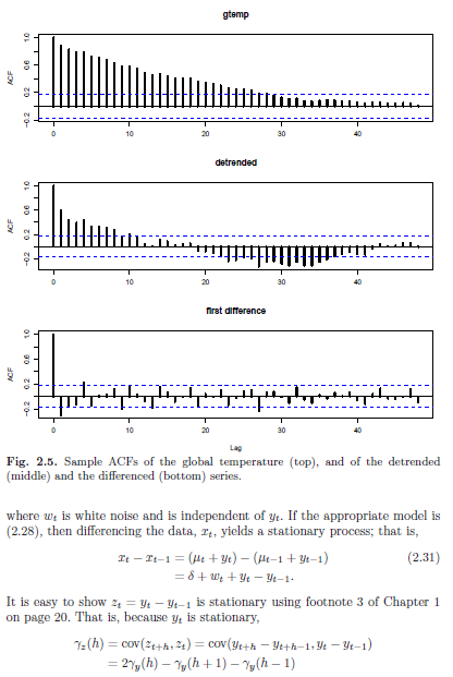
Differencing vs Detrending
- Differencing requires no parameter, BUT it does not yield an estimate of the stationary process yt as can be seen in 2.31.
- Detrending gives an estimate of yt
- Differencing coerce the data to stationarity better and it likes fixed trends.
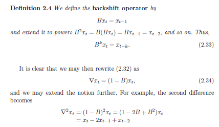
Defintiion 2.5 Diffference of order d
the updown delta to the d power = (1-B)^d
Example 2.5: Differencing Global Temperature
- Differencing the same series- differenced series does not contain long middle cycle
- ACF of this series shows minimal autocorrelation
- global temperature not related to drift
- Fractional differencing - a less-severe operation where d is between -0.5 and 0.5, and then theres a long memory time series where d is between 0 and 0.5. These are often for environmental use
- let yt = log(xt) to equalize the variability over the length of a single series
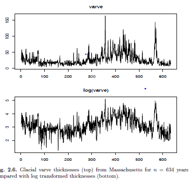
Example 2.6: Paleoclimatic Glacial Varves
- Melting glaciers deposit yearly layers of sand and silt
- We would like to find out variation in thickness as a function of time. And since varation in thickness that increases in proportion to the amount deposited, a logarithmic transformation could remove the nonstationarity observable in the variance as a function of time
- Use:
- par(mfrow=c(2,1))
- plot(varve, main = "varve", ylab="")
- plot(log(varve), main = "log(varve)", ylab="")
Example 2.7: Scatterplot Matrices, SOI, and Recruitment
- Nonlinear relationship is easily conveyed by a lagged scatterplot matrix
- lowess fits are approximately linear
- we want to predict the Recruitment series from current or past values of SOI series. We do that by running the aforementioned tests that will show us periodic behavior in time series data and etc
Example 2.7: Scatterplot Matrices, SOI, and Recruitment
- Nonlinear relationship is easily conveyed by a lagged scatterplot matrix
- we can see some non-linear trend line by plotting the scatterplot and some kind of coefficient will show up indicating the correlation
- we want to predict the Recruitment series from current or past values of SOI series.
Example 2.8: Using Regression to Discover a Signal in Noise
-
set.seed(1000)
x = 2cos(2*pi*1:500/50 + .6*pi) + rnorm(500,0,5)
z1 = cos(2*pi*1:500/50); z2 = sin(2*pi*1:500/50)
summary(fit <- lm(x~0 + z1 + z2))
plot.ts(x, lty = "dashed")
lines(fitted(fit), lwd=2)- this code is used to replicate the usual linear regression on a set of data. If we use a known frequency and "backtrack" to figure out the amplitude and the phase "phi", we can see how close the parameters are and we can find signals from a noise
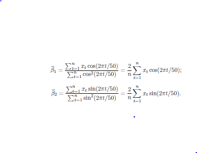
Example 2.9: Using a Periodogram to Discover a Signal in Noise
- but what if we don't know the value of the frequency parameter w ("omega"), if we don't know w, we could try to fit the model using nonlinear regression
- Here's how to get the estimated regression coeff:
"SmoothING"
- concept of smoothing a time series
- we want to specifically smooth white noise and it will help with spotting long term trends
TimeSeriesAnalysisCH2
By tsunwong625


