


Vedant Puri
PhD student at Carnegie Mellon University
Mechanical Engineering, Carnegie Mellon University
Advisors: Prof. Burak Kara, Prof. Jessica Zhang
Motivation
Potential solutions
Computer vision community has been developing fast training architectures
Multi-resolution and sparse architectures that capture high frequency features
Applications
Next steps
Research Plan
Advantages
Disadvantages
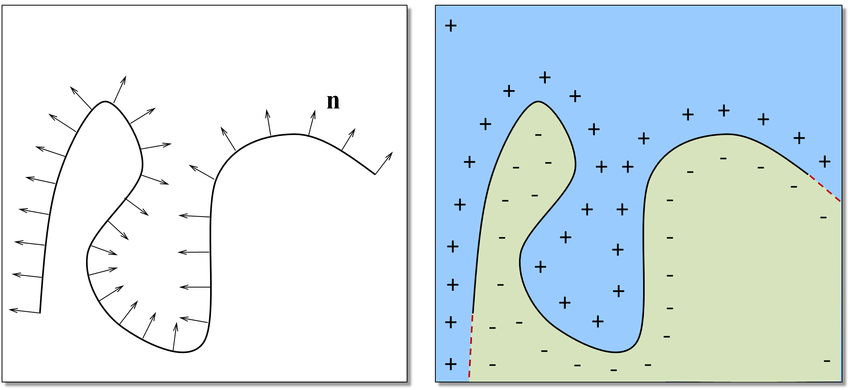
Signal
MLP
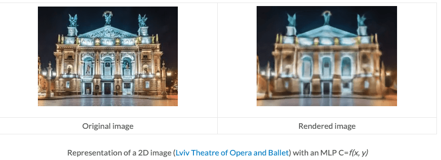
Example: Image regression with deep neural network \( (r, g, b) = NN(x, y) \)
https://www.it-jim.com/blog/nerf-in-2023-theory-and-practice/
https://arxiv.org/pdf/2309.15426
Key idea
Applications
Disadvantages
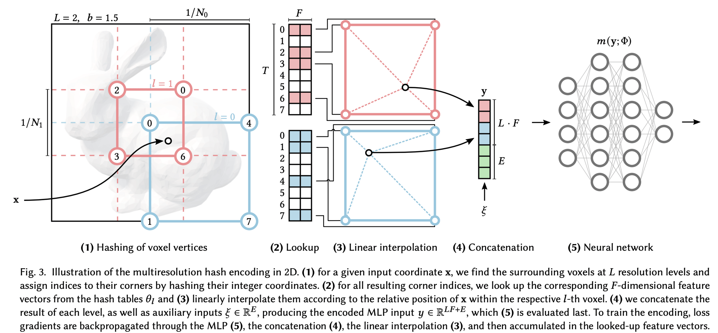
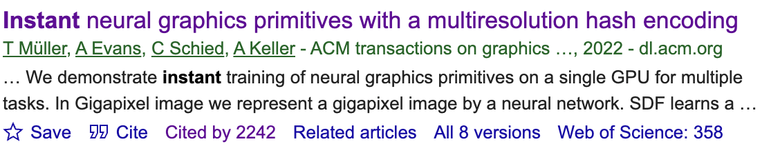
Instant neural graphic primitives with multiresultion hash encoding 2022
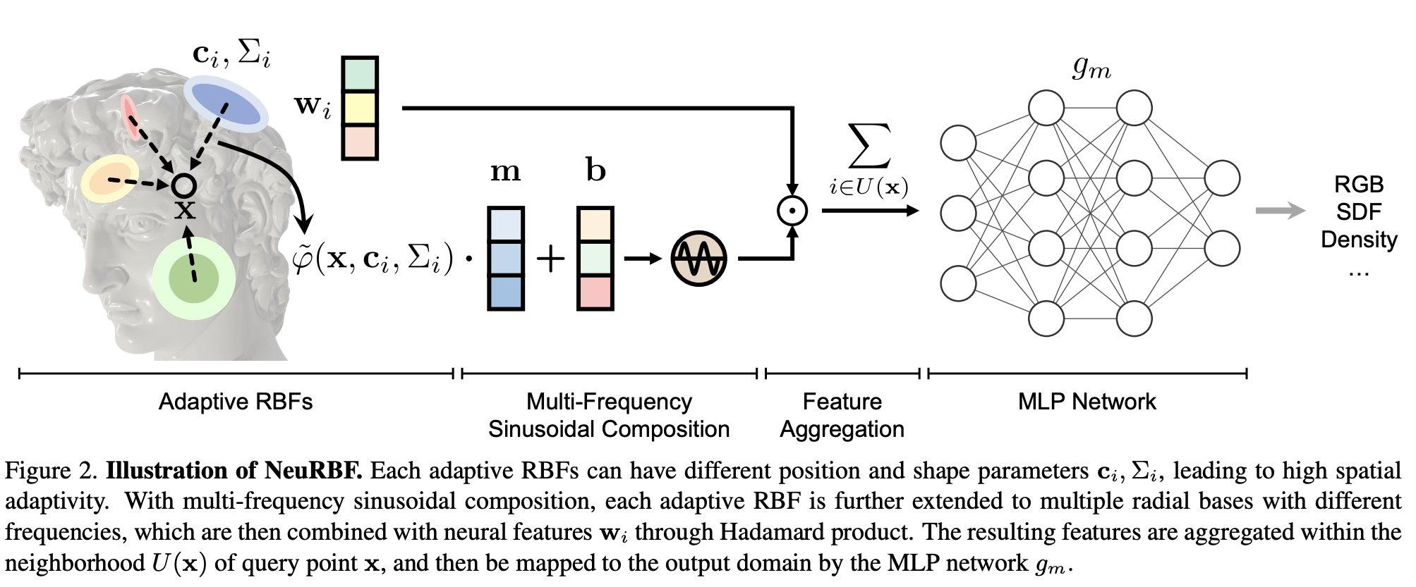
NeuRBF: A Neural Fields Representation with Adaptive RBF 2023
The Thirty-Eighth AAAI Conference on Artificial Intelligence (AAAI-24)
| Method | Approach | Notes |
|---|---|---|
| Instant NGP 2022 | Learn multiple overlapping feature grids at different resolutions | Leads to sharp gradients at grid boundaries |
| 3D Gaussian splating 2023 | No neural network. Parameterize solution as sum of gaussians with learnable position, covariance. Adaptively add/rm gaussians. | Easier PINNs optimization problem since theres no NN? |
| NeuRBF 2023 | Adaptive RBF feature grid | RBF features are smoothly interpolated |
| Dictionary fields 2023 | ||
| Plenoxels | ||
| TenosRF |
Many important papers in this field
Mechanical Engineering, Carnegie Mellon University
Advisors: Prof. Burak Kara, Prof. Jessica Zhang
Motivation
Potential solutions
Multi-resolution and sparse architectures developed by CV community train in minutes rather than days
Would need to be modified to fit physics problems
Research problem
PMFI project
Current state of ML-ROM
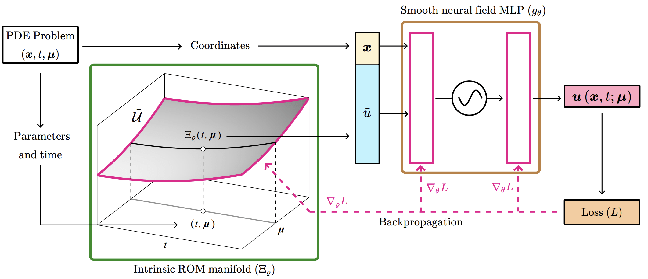
(SNF-ROM, 2024)
PMFI proposal
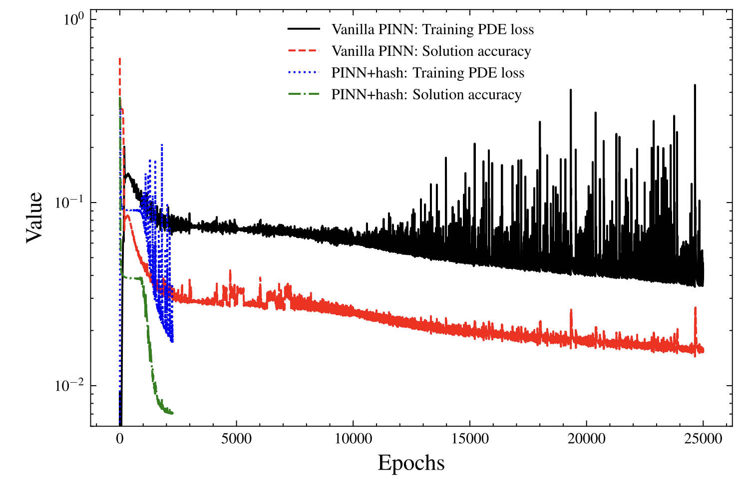
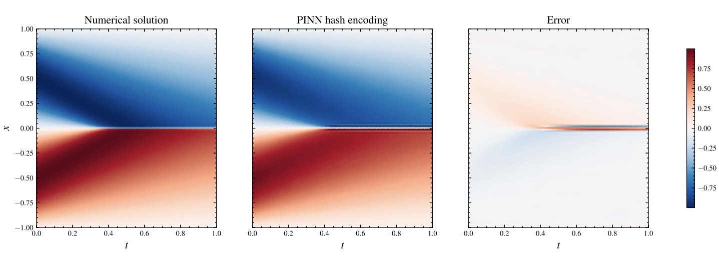
Current state of PINNs (NSFnet 2020)
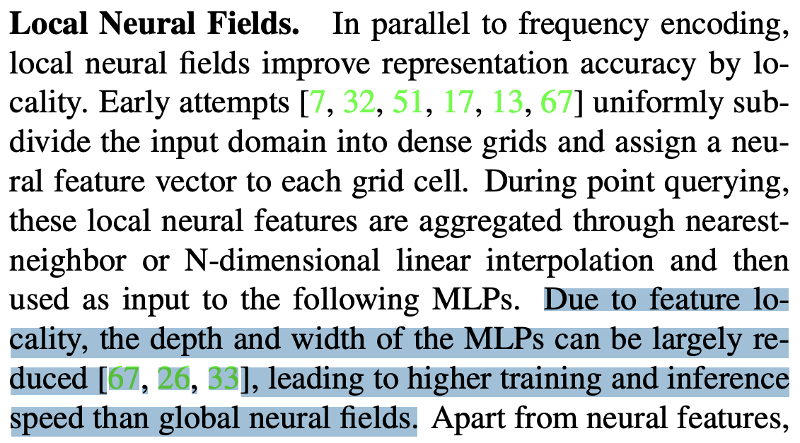
Neural field MLP
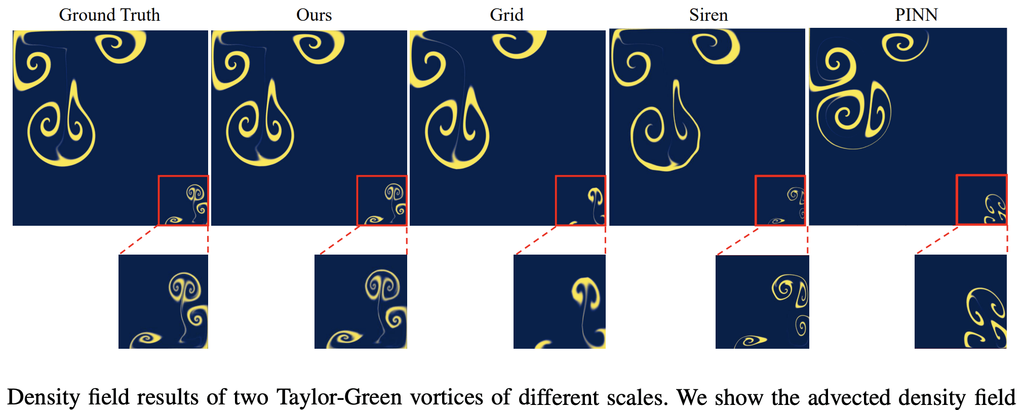
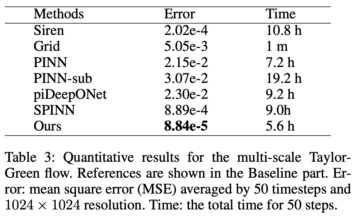
Multiresolution architectures
Instant neural graphic primitives with multiresultion hash encoding 2022
| Method | Approach | Notes |
|---|---|---|
| Instant NGP 2022 | Learn multiple overlapping feature grids at different resolutions Hash encoding for fast querying |
Applied to PINNs for simple problems. Leads to sharp gradients at grid boundaries |
| 3D Gaussian splatting 2023 | No neural network. Parameterize solution as sum of gaussians with learnable position, covariance. Adaptively add/rm gaussians. | Explicit representation can lead to easier PINNs optimization problem since there's no NN? |
| NeuRBF 2023 | Combination of adaptive RBF and grid RBF features. Sinusoidal composition for multi-freq. Similar to 3DGS but no adaptive control. | RBF features are smoothly interpolated. Very desirable. Possibly good for PINNs. |
| Dictionary fields 2023 | factorize a signal into a coefficient field and a basis field which is a dictionary of known functions. use coordinate transformations to apply the same basis functions across multiple locations and scales, typically in a grid pattern. | Combines deterministic functions with learned coefficient fields. Can we control smoothness? Grid structure can lead to large number of parameters. |
Motivation
Potential solutions
Develop fast training multi-resolution architectures
Would need to be modified to fit physics problems
New contribution
Research plan
PMFI Project
This week
Set up learning pipeline for Task 2.1 with toy dataset for a small neural network
Finished literature review
Start implementing state of the art models next week
PMFI proposal
PMFI Project
This week
Finished setting up learning pipeline for Task 2.1 with toy dataset for a small neural network
Finished literature review on ML architectures for task 2.1
Start implementing state of the art models next week
Goal
Task 1 - Data generation
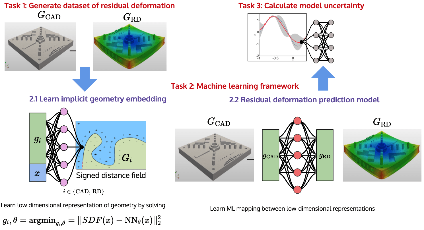
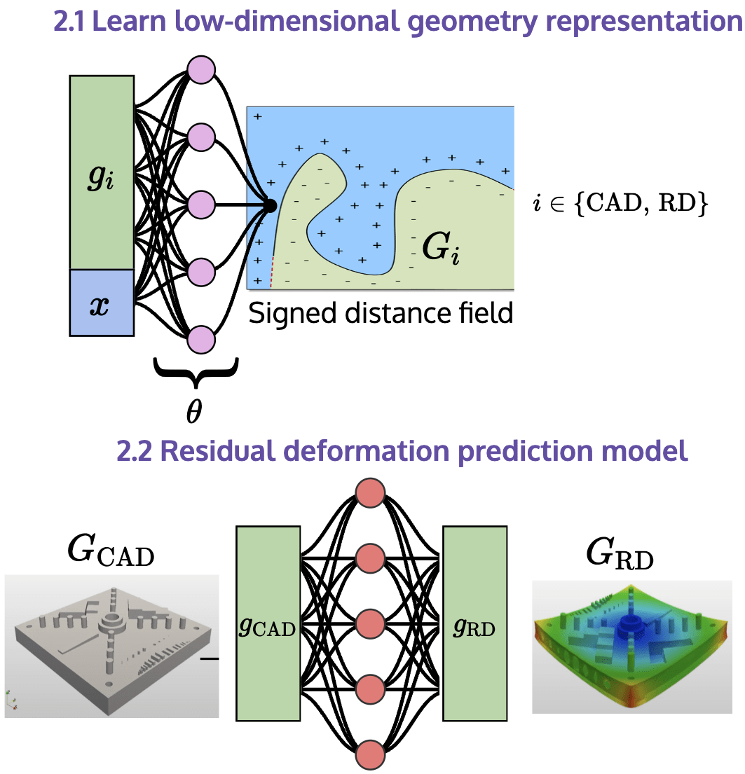
Task 2.1 - Dimensionality reduction
Task 2.2 - Surrogate model
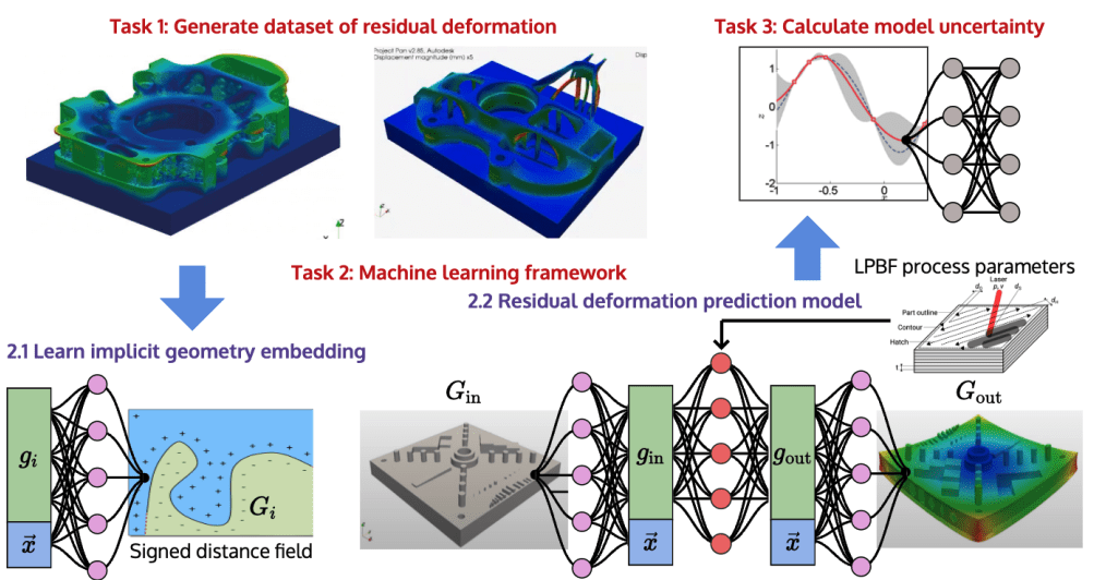
PMFI Project Goal
Task 1 - Data generation
Task 2.1 - Dimensionality reduction
Task 2.2 - Predict residual deformation
New Contributions
Task 1 - Generate dataset of residual deformation calculations
This week
Task 1 - Generate dataset of residual deformation calculations
Task 2 - ML Surrogate model
New contributions
APDL Code
NetFabb Simulations
Shape reconstruction with baseline method (MLP)
PMFI Project Goal
Task 1 - Data generation
Task 2.1 - Dimensionality reduction
Task 2.2 - Predict residual deformation
New Contributions
Reviewer 1
Reviewer 2
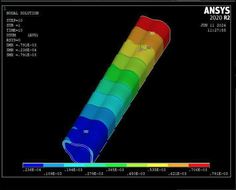
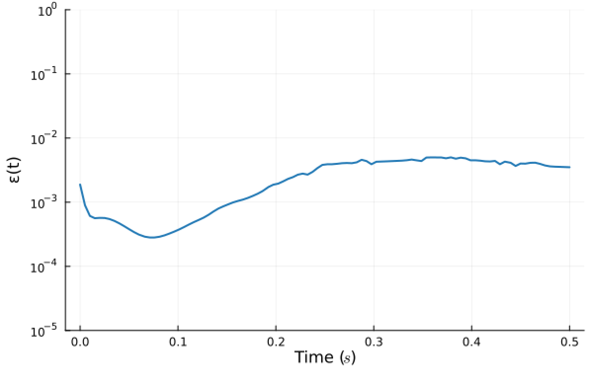
FOM: 15.530123 seconds (GPU allocations: 163.760 GiB)
ROM:  0.862563 seconds (GPU allocations:   8.925 GiB)
Burgers 2D - Error vs time plots
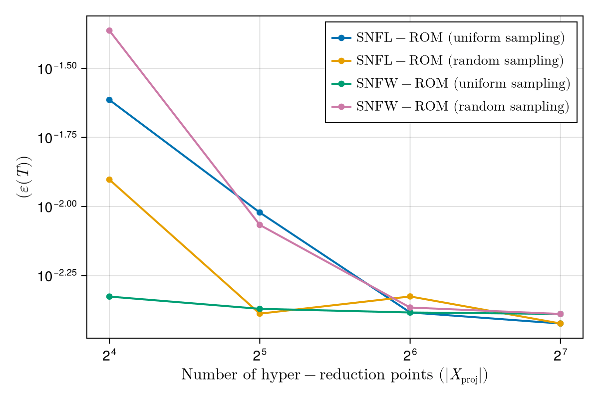
No hyper-reduction
with hyper-reduction
ROM w. large DT: 0.157669 seconds (GPU allocations: 1.790 GiB)hyper-reduction + large \(\Delta t\)
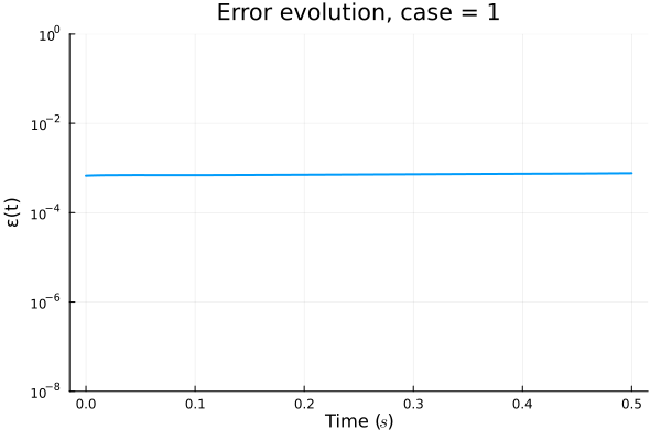
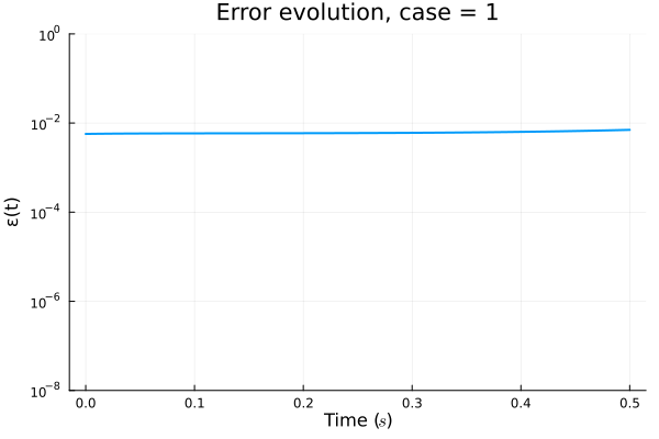
\(1 \%\) error
\(1 \%\) error
\(1 \%\) error
Reviewer 1
Reviewer 2
Plan
Mechanical Engineering, Carnegie Mellon University
Advisors: Prof. Burak Kara, Prof. Jessica Zhang
WCCM Conference Takeaways
Offline stage
Online stage
Plan for upcoming projects
Fundamental ROM project
Based on discussions at WCCM, I have devised a plan to address current limitations of SNF-ROM
PMFI project
Earlier consensus was to use Kevin's work to satisfy grant requirements
In more recent discussions, Prof. Zhang indicated she wants at least a paper report back to PMFI in recent discussions
Prof. Zhang has also pointed out some other opportunities in geometry modeling
Question
Offline stage
Online stage
Motivation
Address current limitations: long training times, limited accuracy
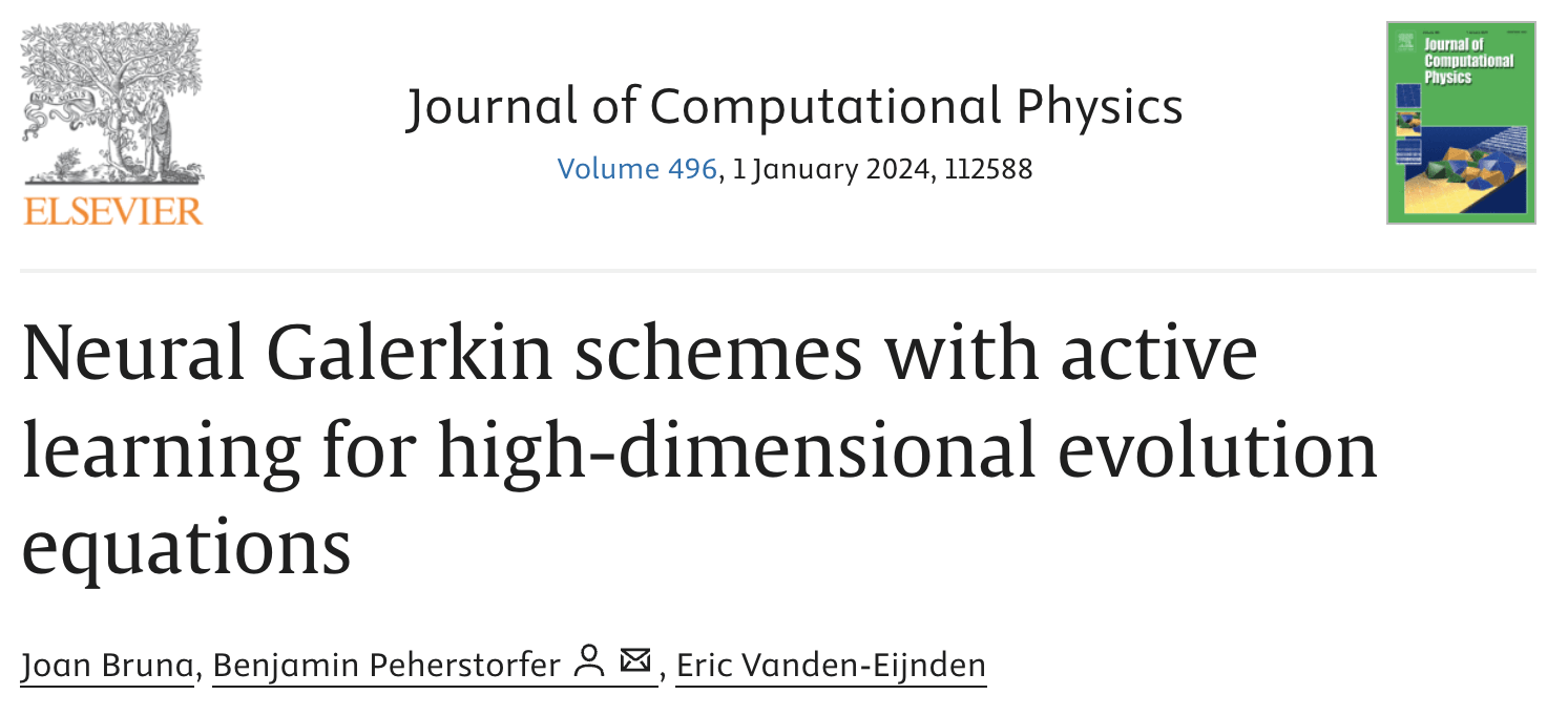
NYU group led by Benjamin Peherstorfer.
First paper (Mar 2022). 43 citations thus far
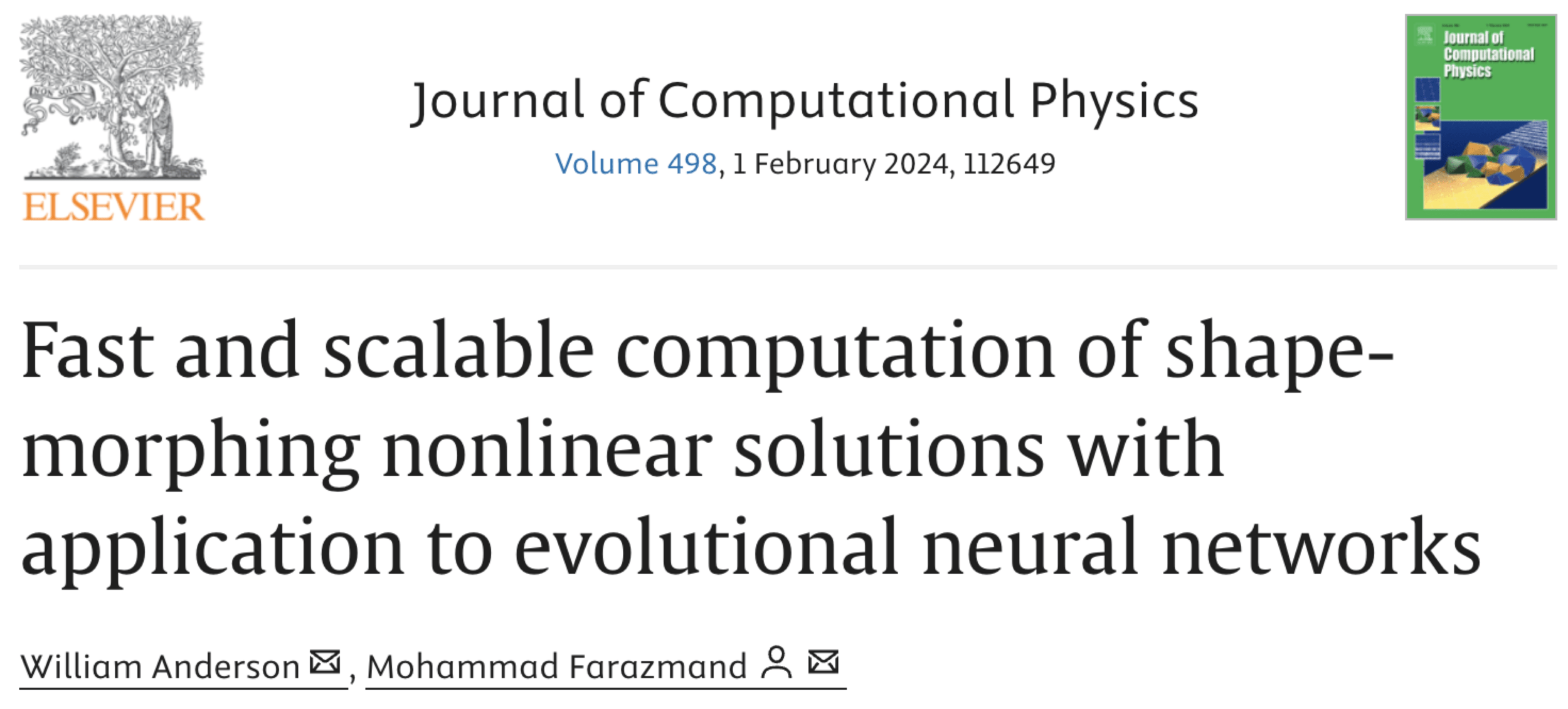
William Anderson (PhD NC State, Post-doc at LANL)
Our unique edge
Our unique edge
ROM project (Neural Galerkin)
PMFI Project / Geometry modeling
Neural Galerkin method
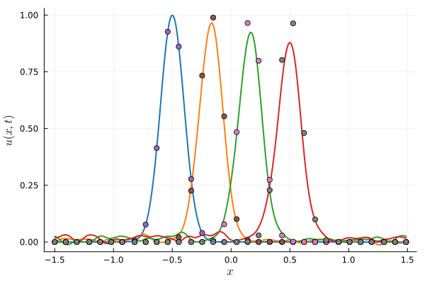
Deep Neural Network (BASELINE)
~150 parameters
256 collocation points
Multiplicative filter network (MFN)
~210 parameters
256 collocation points
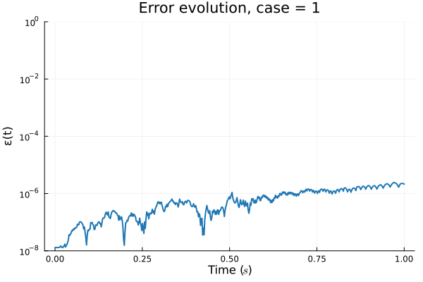
Machine precision accuracy with exact solution
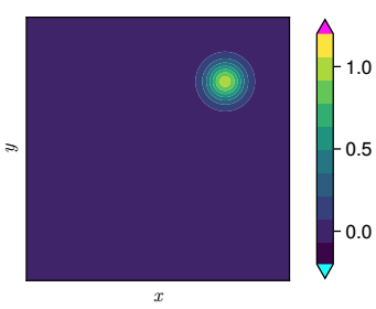
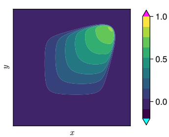
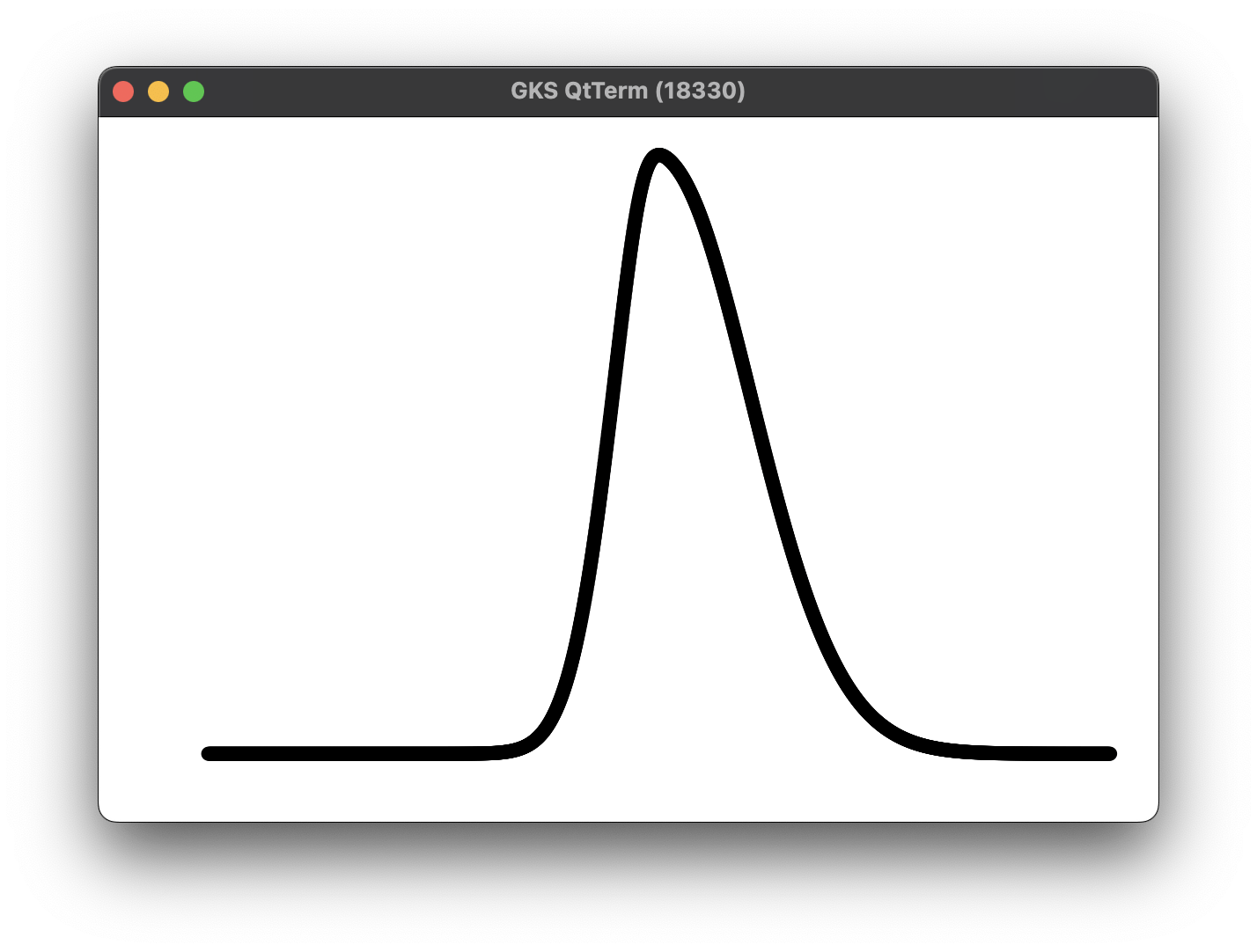
Parameterized Gaussian (OURS)
3 parameters
8 collocation points
Fast evaluation!
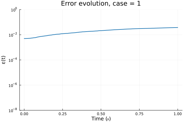
Deep Neural Network (BASELINE)
~150 parameters
256 collocation points
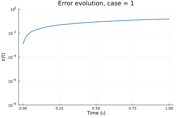
Multiplicative filter network (MFN)
~210 parameters
256 collocation points
Error due to limited expressivity of this simple model
Parameterized Gaussian (OURS)
3 parameters
8 collocation points
Parameterized Gaussian (OURS)
3 parameters
8 collocation points
Deep Neural Network (BASELINE)
~150 parameters
256 collocation points
Multiplicative filter network (MFN)
~210 parameters
256 collocation points
Error due to limited expressivity of this simple model
FAILED TO CONVERGE
Conclusions from "proof of concept" experiment
Next steps
Sources of error in experiment
Potential New Contributions
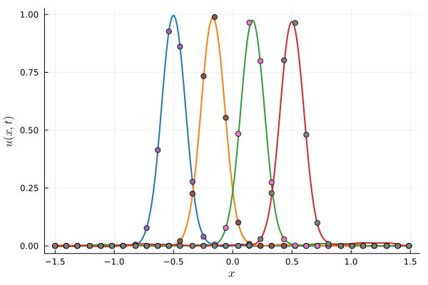
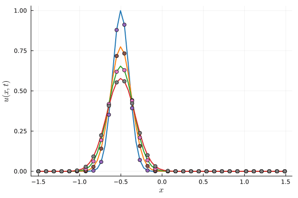
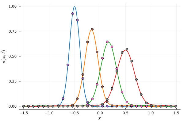
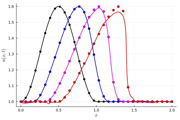
Time-integration of Parameterized Gaussian (OURS)
Parameterized Gaussian discretization
Updates
Next steps
Potential new contributions
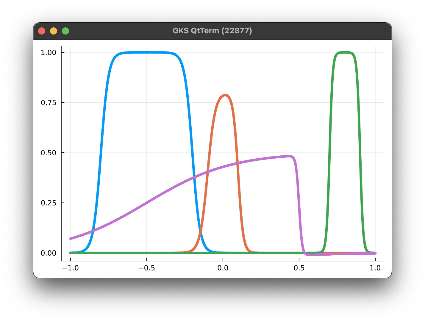
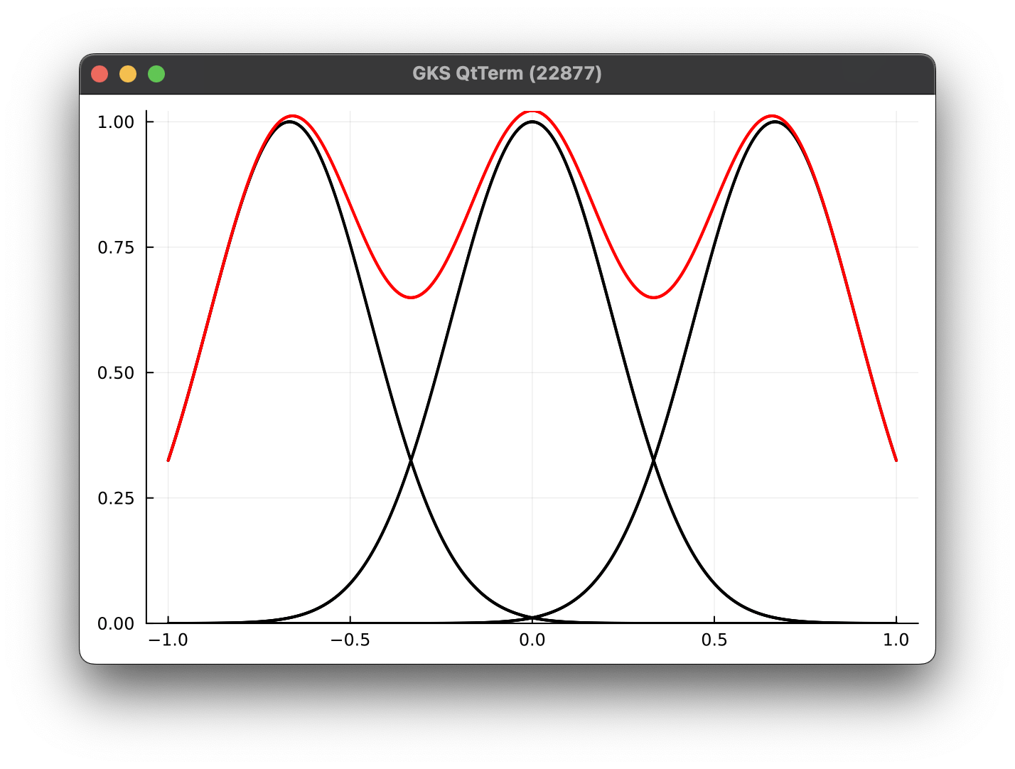
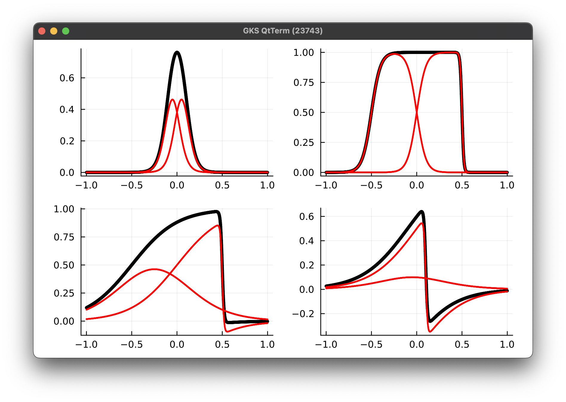
Parameterized Gaussian kernels
Multiple parameterized Gaussians kernels
Multiple parameterized Gabor kernels
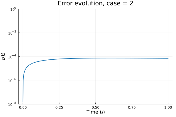
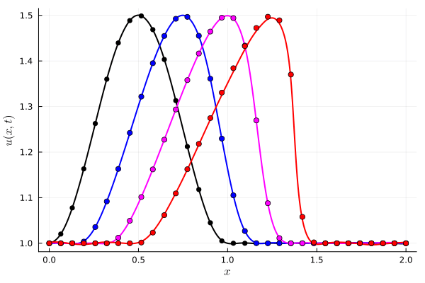
Parameterized Gaussian (OURS)
8 parameters, 512 collocation points
Compute time: \(0.17~\text{s}\)
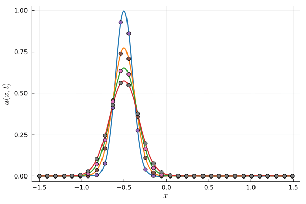
Deep Neural Network (BASELINE)
~150 parameters, 512 collocation points
Compute time: \(6~\text{s}\)
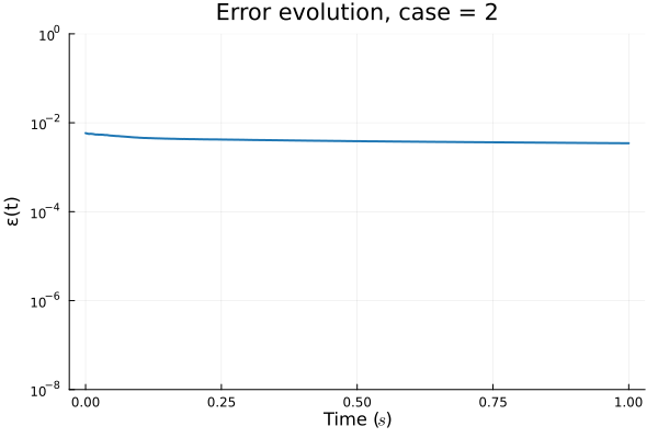
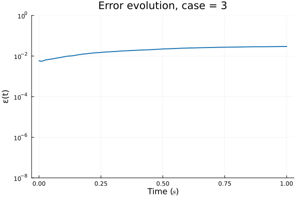
Accuracy limited by initial projection step
Parameterization
FOM compute time: \(0.80~\text{s}\)
PMFI Project Goal
Task 1 - Data generation
Task 2 - Formulate dynamics problem problem
Task 1: AM process simulation with NetFabb
Updates
Next steps
Potential new contributions
Parameterized Gaussians kernels
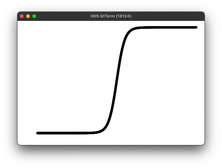
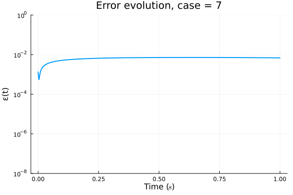
Parameterized Tanh kernels
Gaussian kernels
Tanh kernels
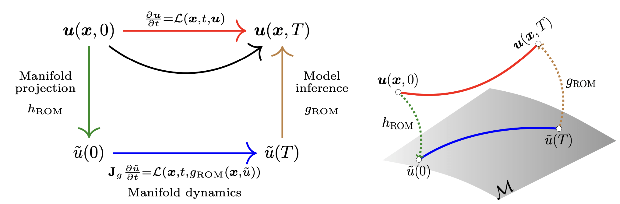
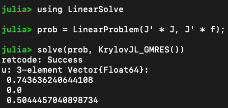
Governing PDE
Ansatz
Galerkin projection
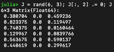
Problem
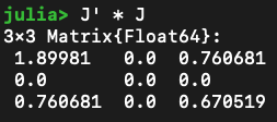
\(\mathbf{J}_g\) can be rank deficient
\(\implies\) Ill-behaved system solve
QR factorization would silently fail and return either NaNs or \(\begin{bmatrix}0 & \cdots & 0 \end{bmatrix}\)
Iterative solvers can invert rank-deficient systems and return a non-unique solution
This has been causing instability in online solve for complicated paramterizations
Solution
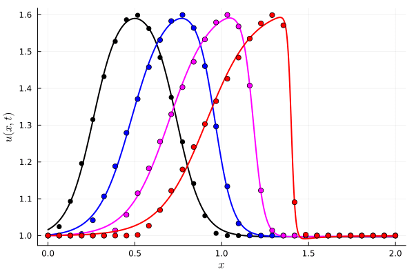
Parameterized Tanh (OURS): 6 parameters, 8192 collocation points
Deep Neural Network (BASELINE): ~150 parameters, 8192 collocation points
FOM compute time: \(7~\text{s}\)
DNN compute time: \(10~\text{s}\)
Our compute time: \(0.07~\text{s}\)
PMFI Project Goal
Task 1 - Data generation
Task 2 - Formulate dynamics problem problem
Task 1: AM process simulation with NetFabb
PMFI Project Goal
Our approach
Application
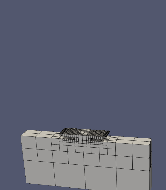
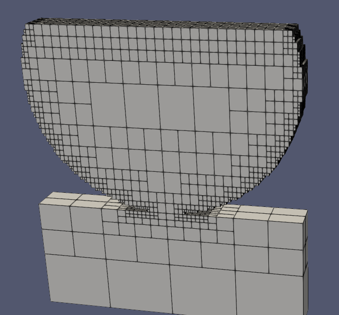
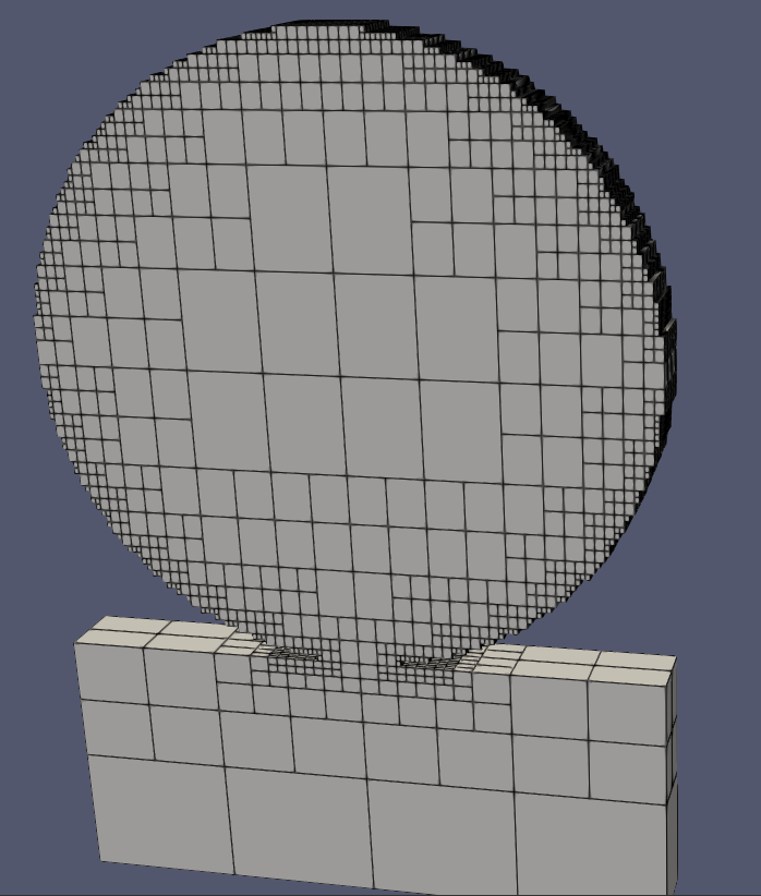
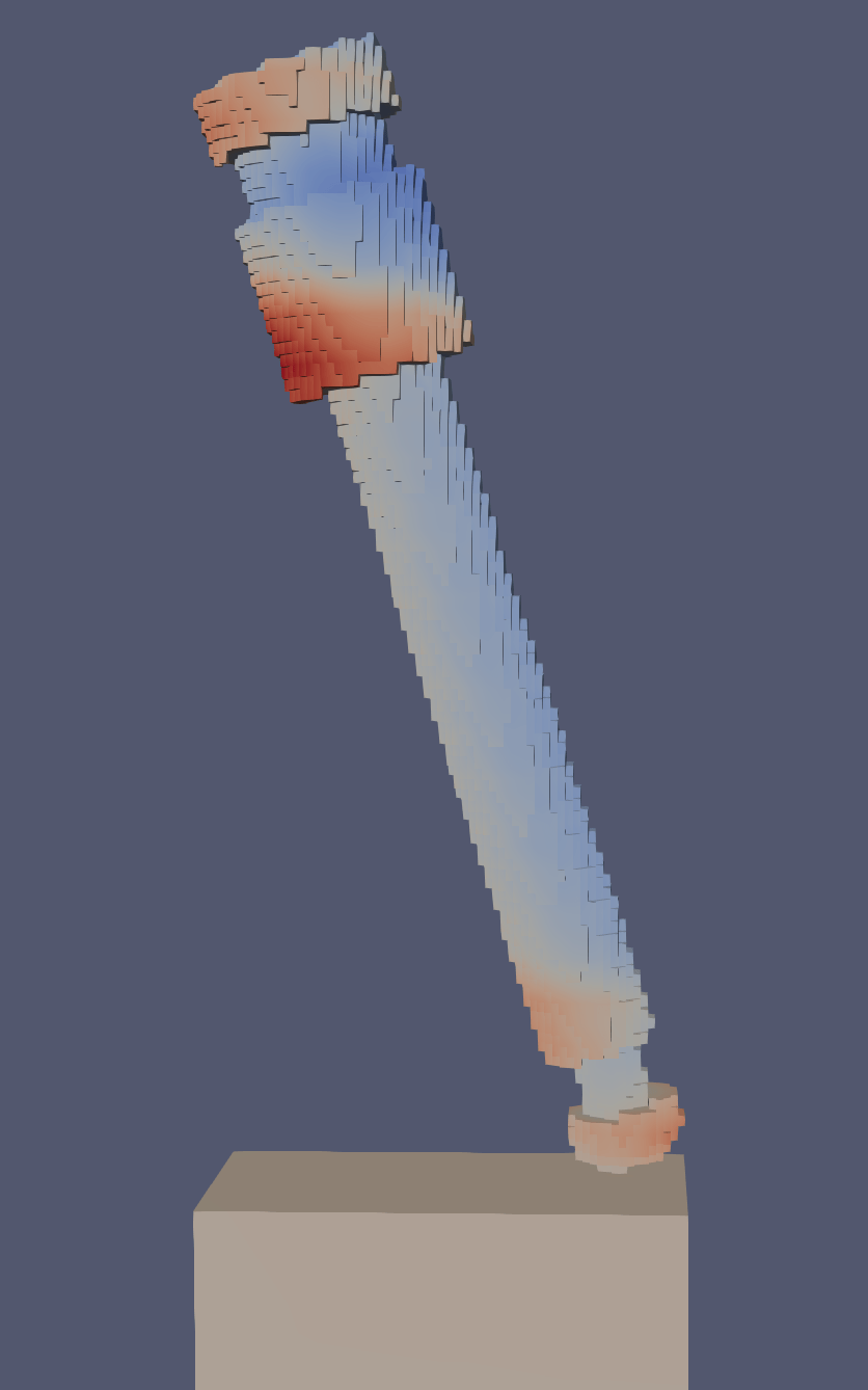
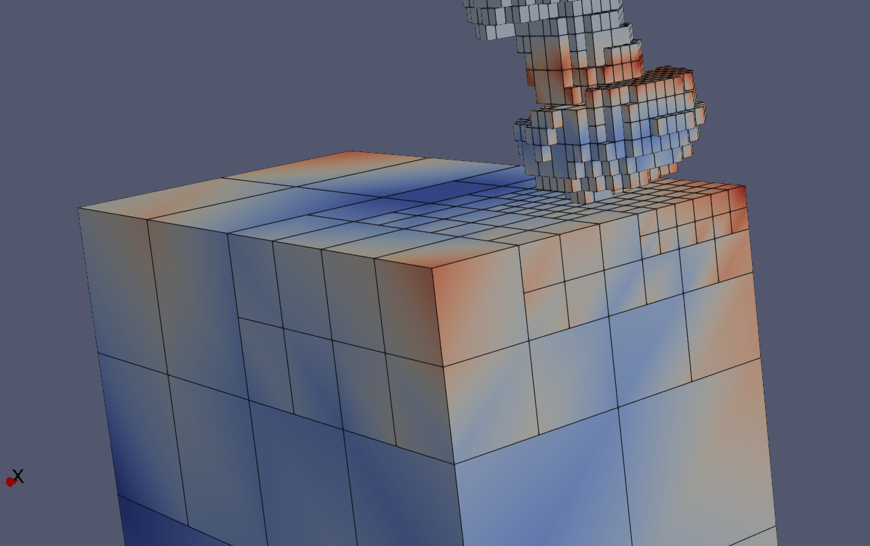
LPBF process simulation with Autodesk NetFabb
CAD = get_CAD_geometry()
displacement = []

for l in 1:num_layers(CAD) # loop over layers

	# slice geometries
	next_cad_layer = CAD[l]
    prev_layer_disp = displacement[1:l-1]

    # our model
    next_layer_disp = predict_layer_disp(next_cad_layer, prev_layer_disp)

	# update Geometry
	displacement.append(next_layer_disp)
end

asbuilt_geometry = CAD + displacement
asbuilt_geometry.visualize()
\(\texttt{CAD[l]}\)
\(\mathrm{NN}\)
\(\texttt{disp[1:l-1]}\)
\(\texttt{disp[l]}\)
Modeling task
\(\texttt{disp[1:l-1]}\)
\(\texttt{CAD[l]}\)
\(\mathrm{NN}\)
\(\texttt{disp[l]}\)
Open questions
Layer L+1
Layer L
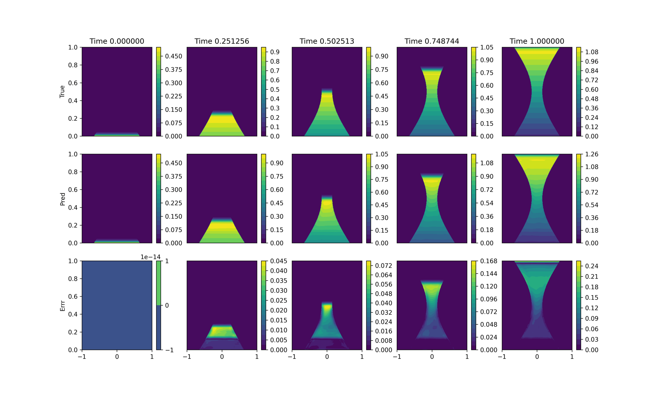
LPBF process simulation with Autodesk NetFabb
Synthetic dataset
LPBF process simulation with Autodesk NetFabb
True
Prediction
Abs Error
temperature_data = get_data()

temperatures = []
temperatures.append(temperature_data[0])

for time in 0:T # loop over time-steps
	curr_temp = temperatures[-1]
    next_temp = CNN(curr_temp, time, X, Z)
    temperatures.append(next_temp)
end
Training
Inference (auto-regressive rollout)
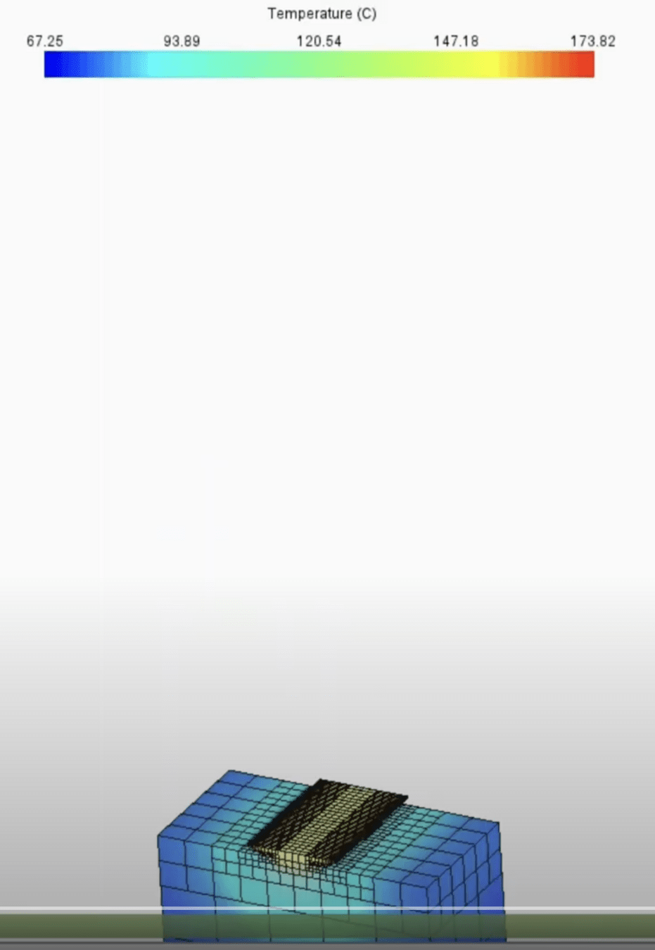
Large errors during training lead to complete deviation during inference
Large errors localized to the interface
This causes discontinuities in the temperature distribution that cannot be captured by CNN/GNN.
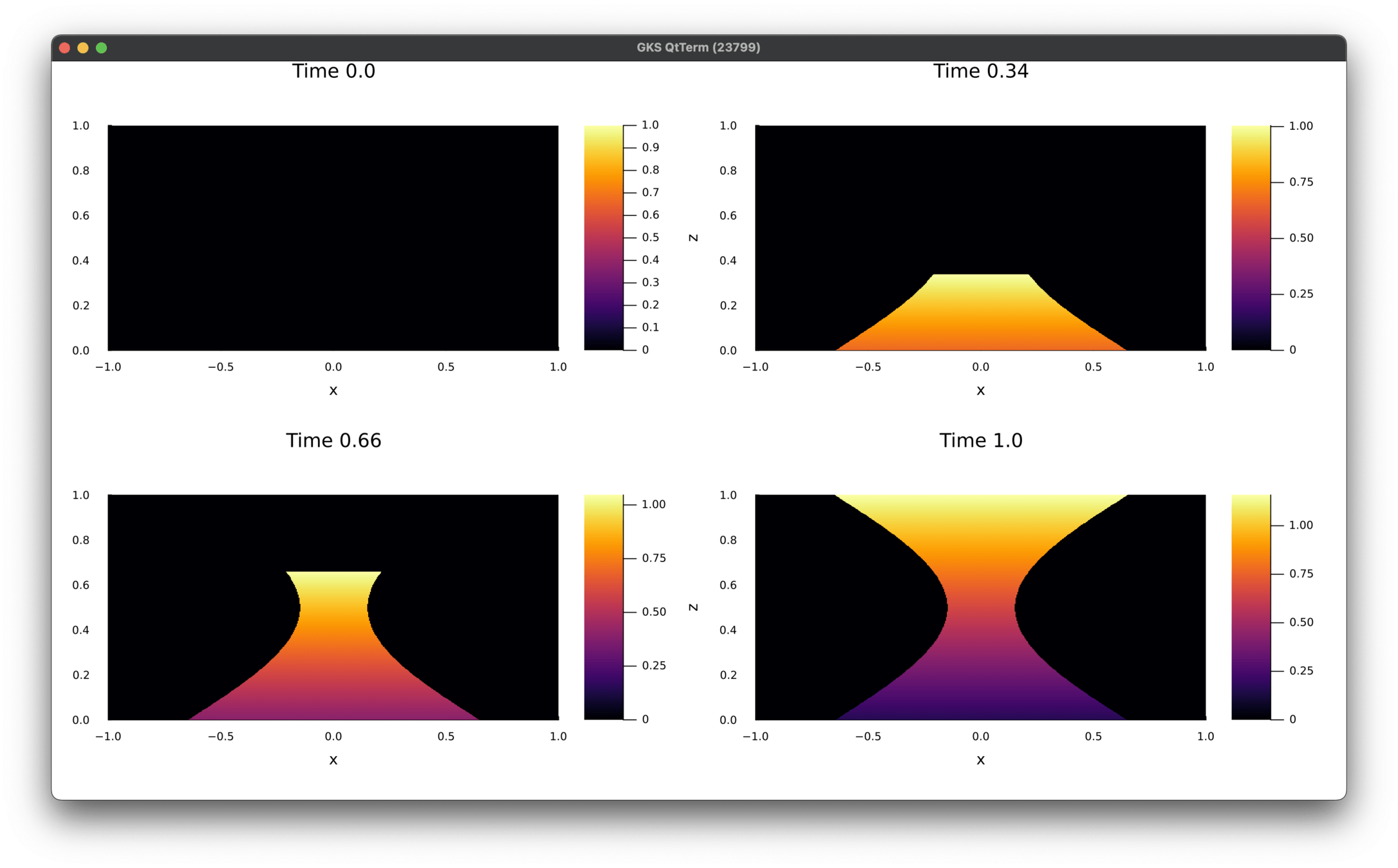
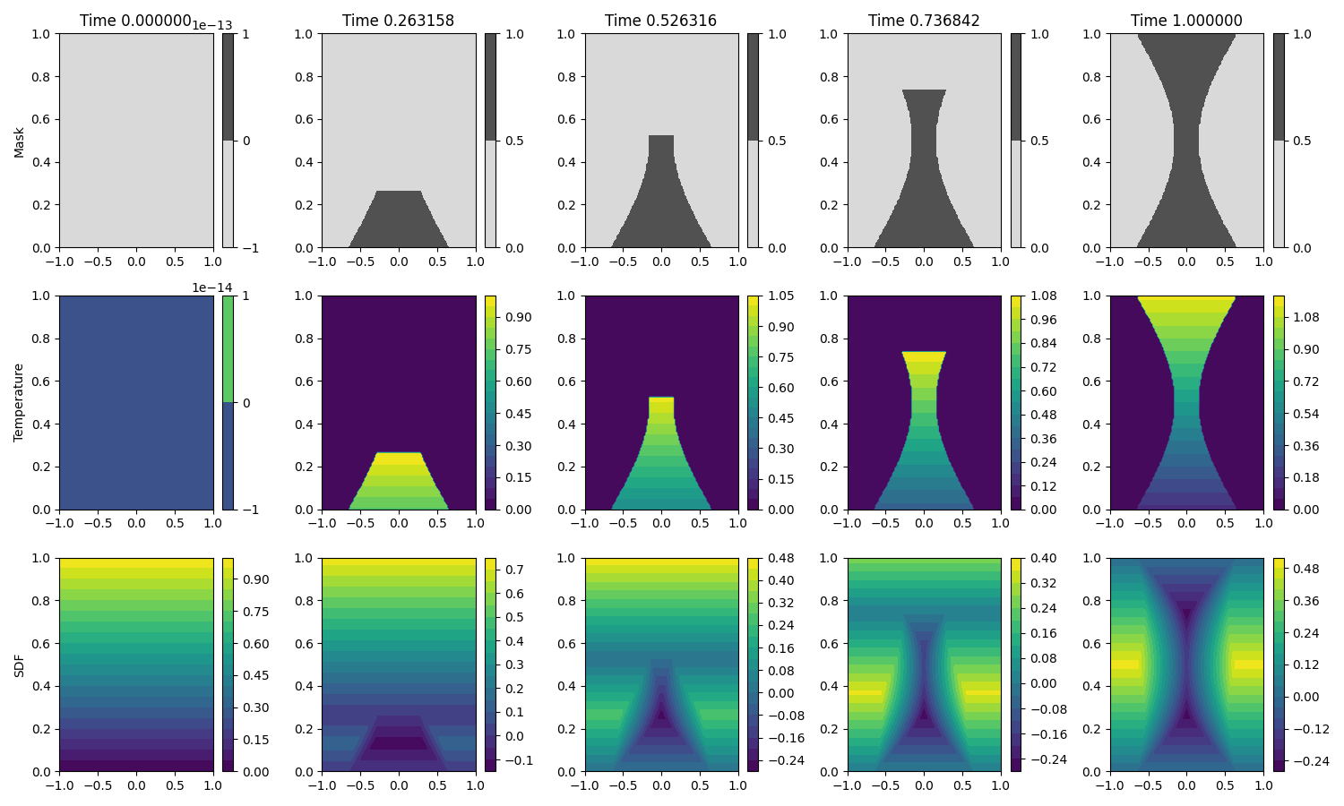
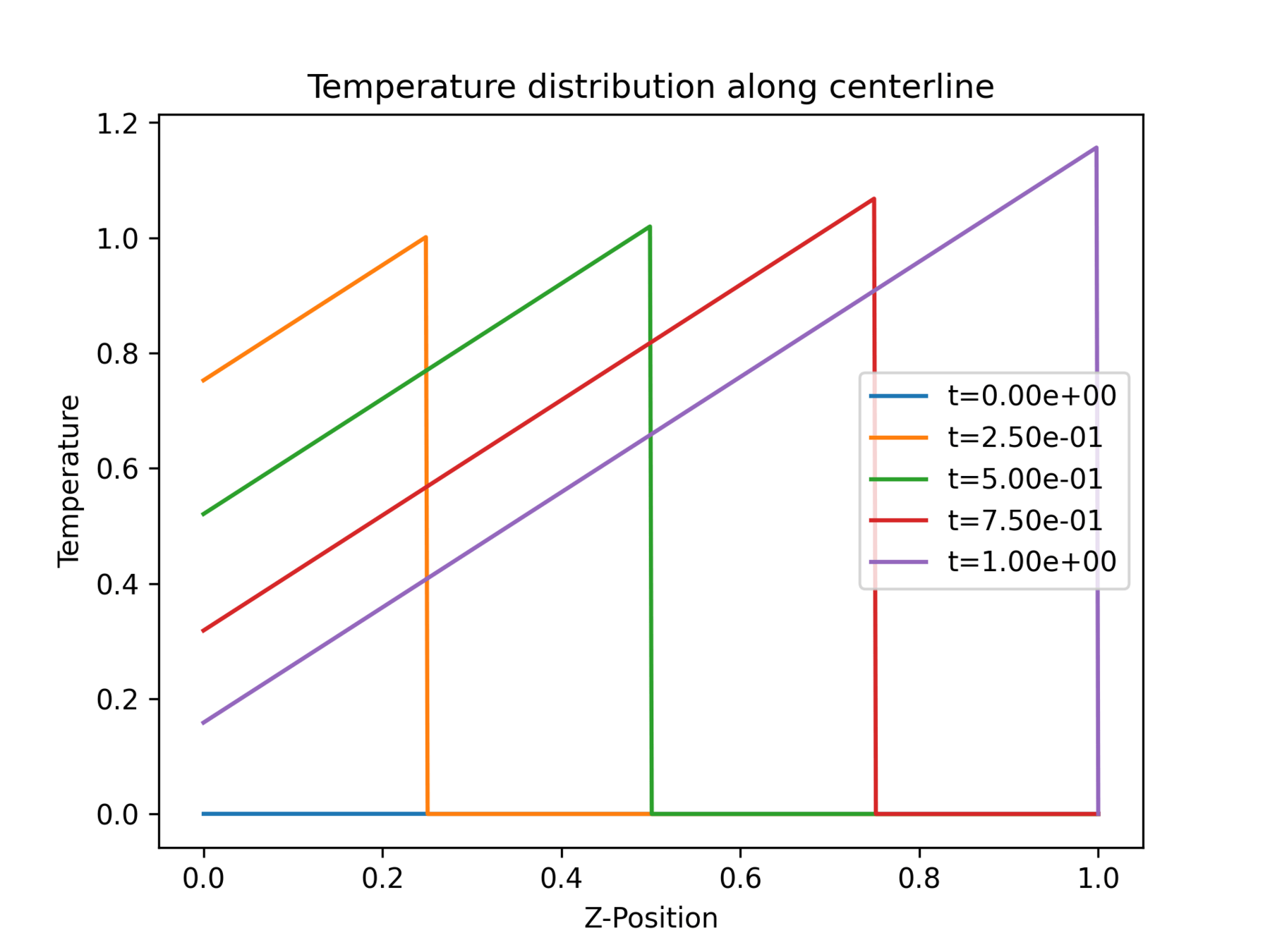
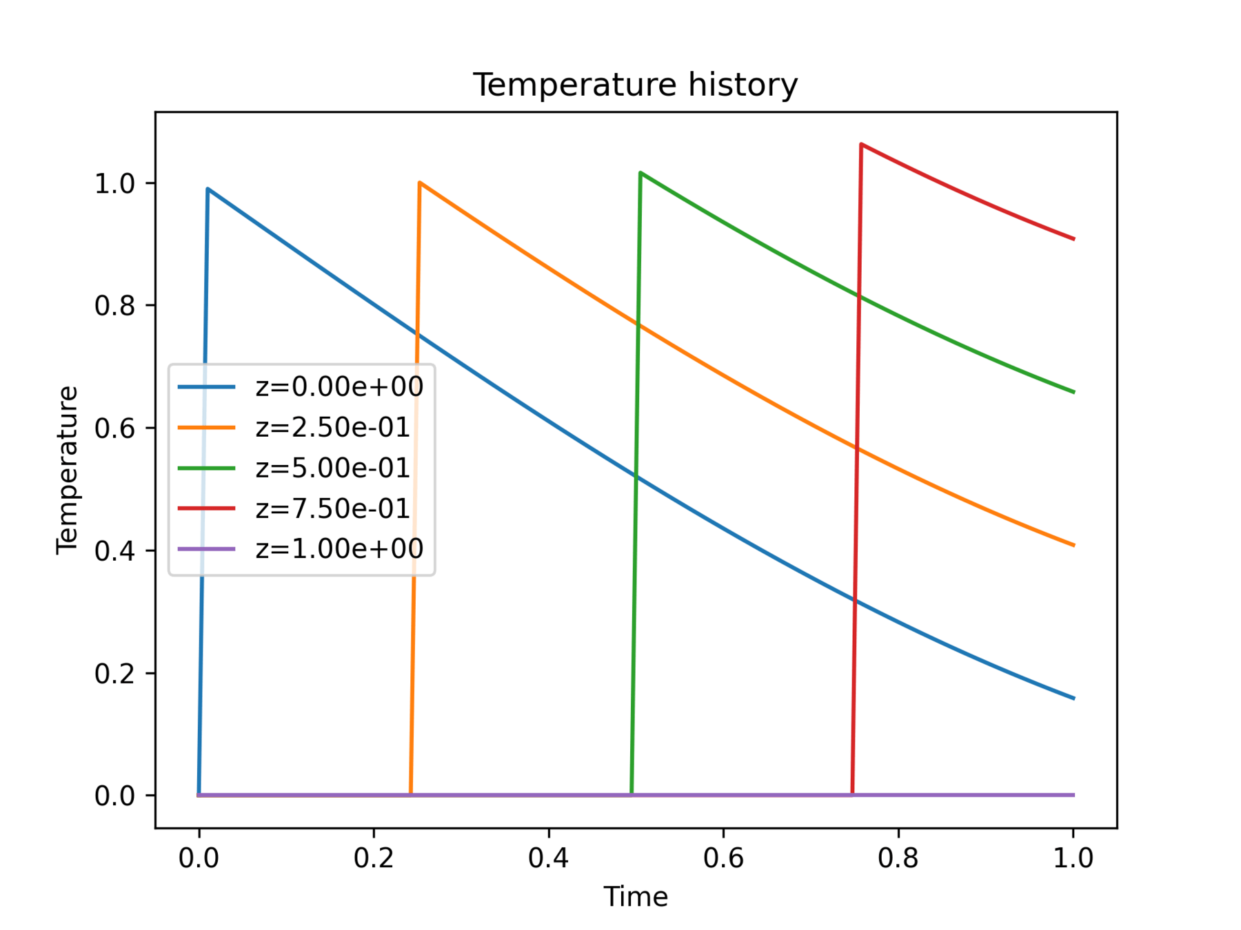
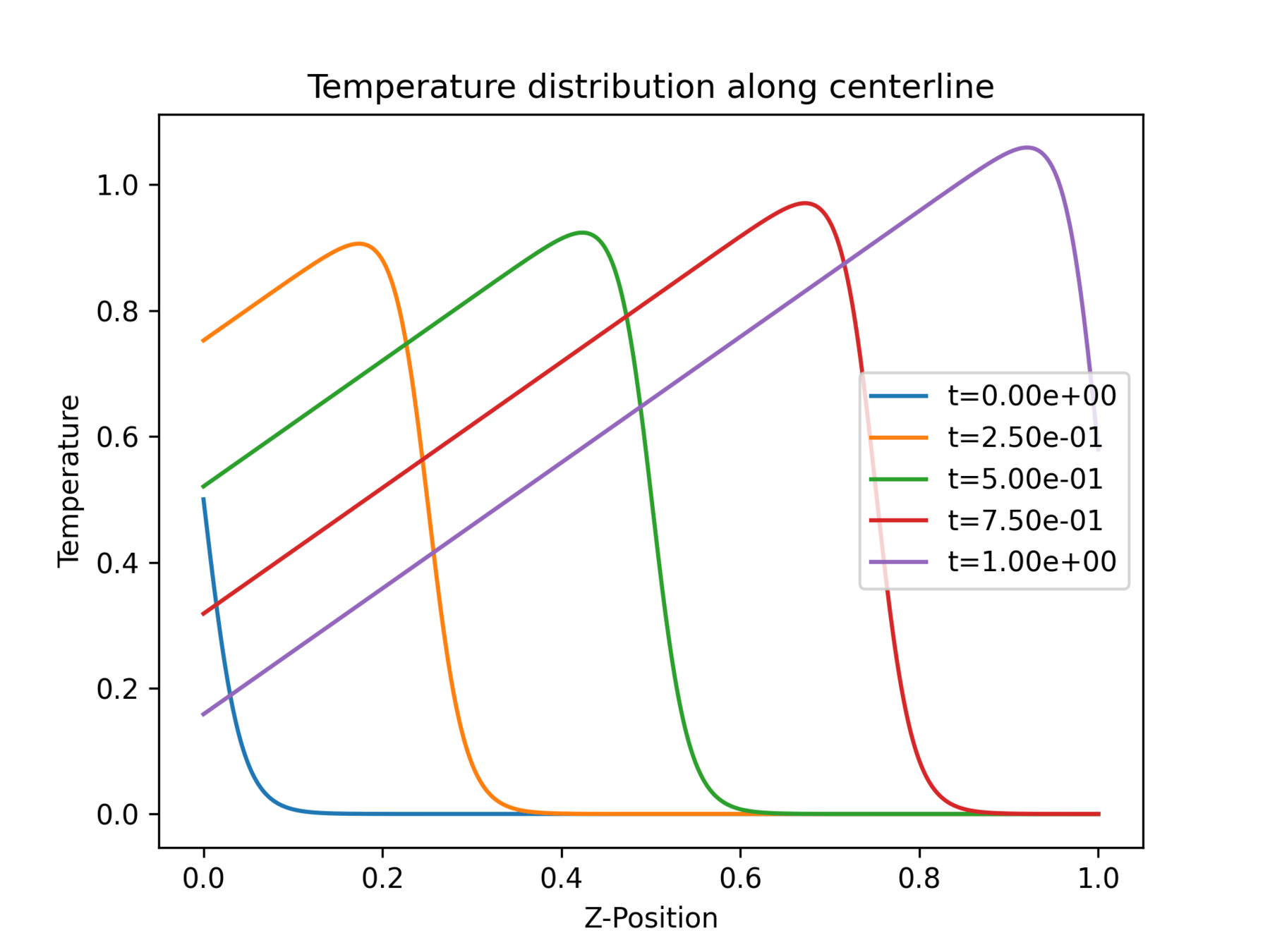
Sandbox was designed to mimic the temperature history of the AM dataset
at a point
True
Prediction
Error
Training
Inference (auto-regressive rollout)
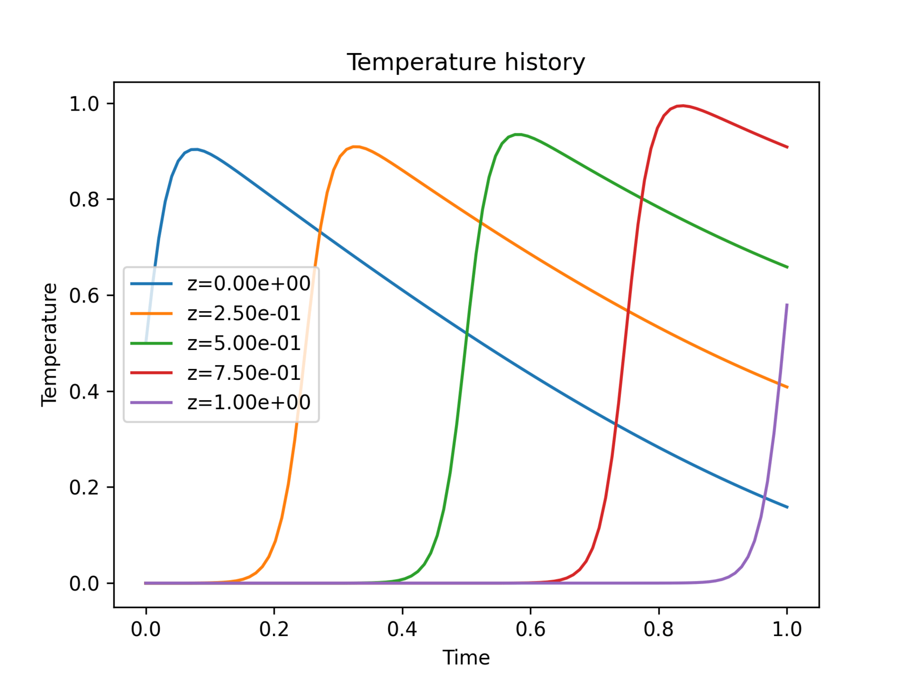
Introduce a blending function to smoothen the discontinuity
Question: Is this representative of the NetFabb dataset?
at a point
Discontinuous
Continuous
Implication:
Implication:
This is not representative of the dataset
This is representative of the dataset
at a point
at a point
2
1
3
1
2
This is not representative of the dataset
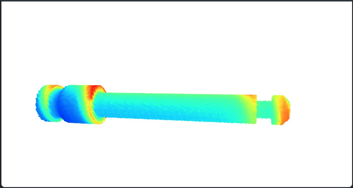
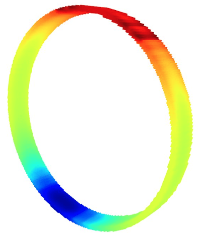
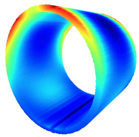
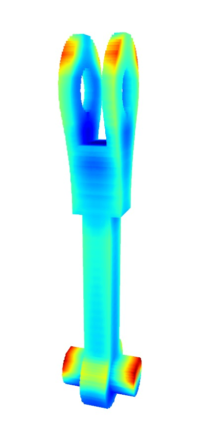
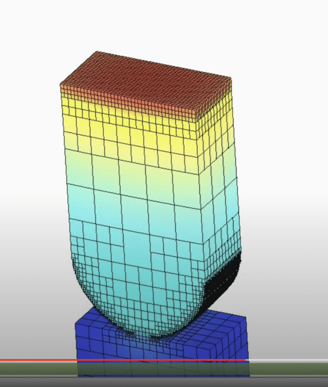
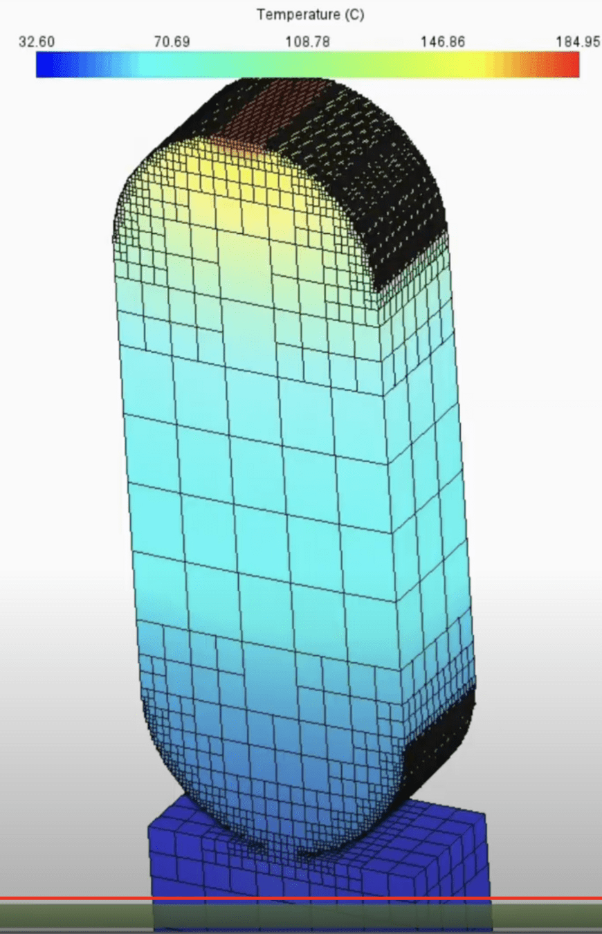
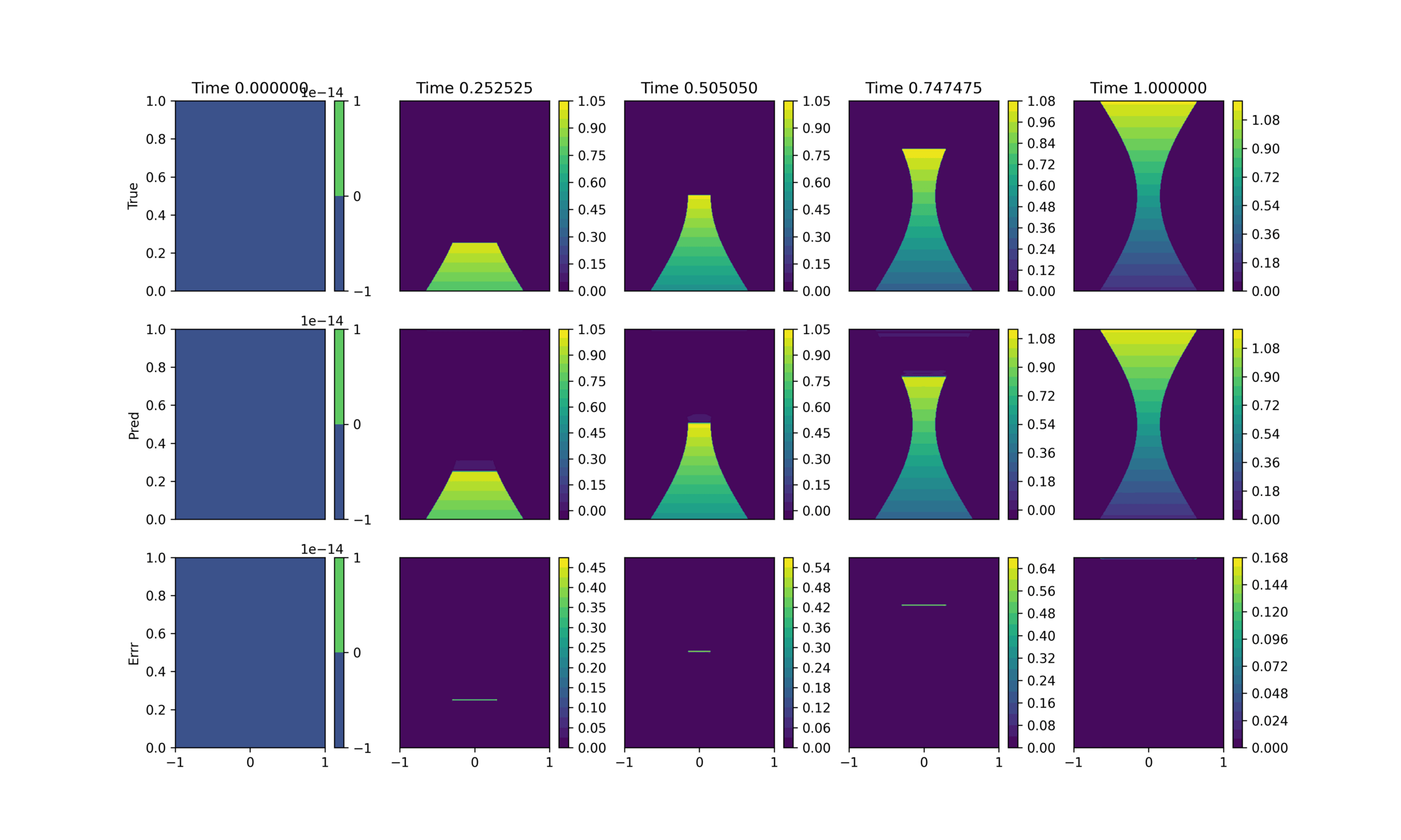
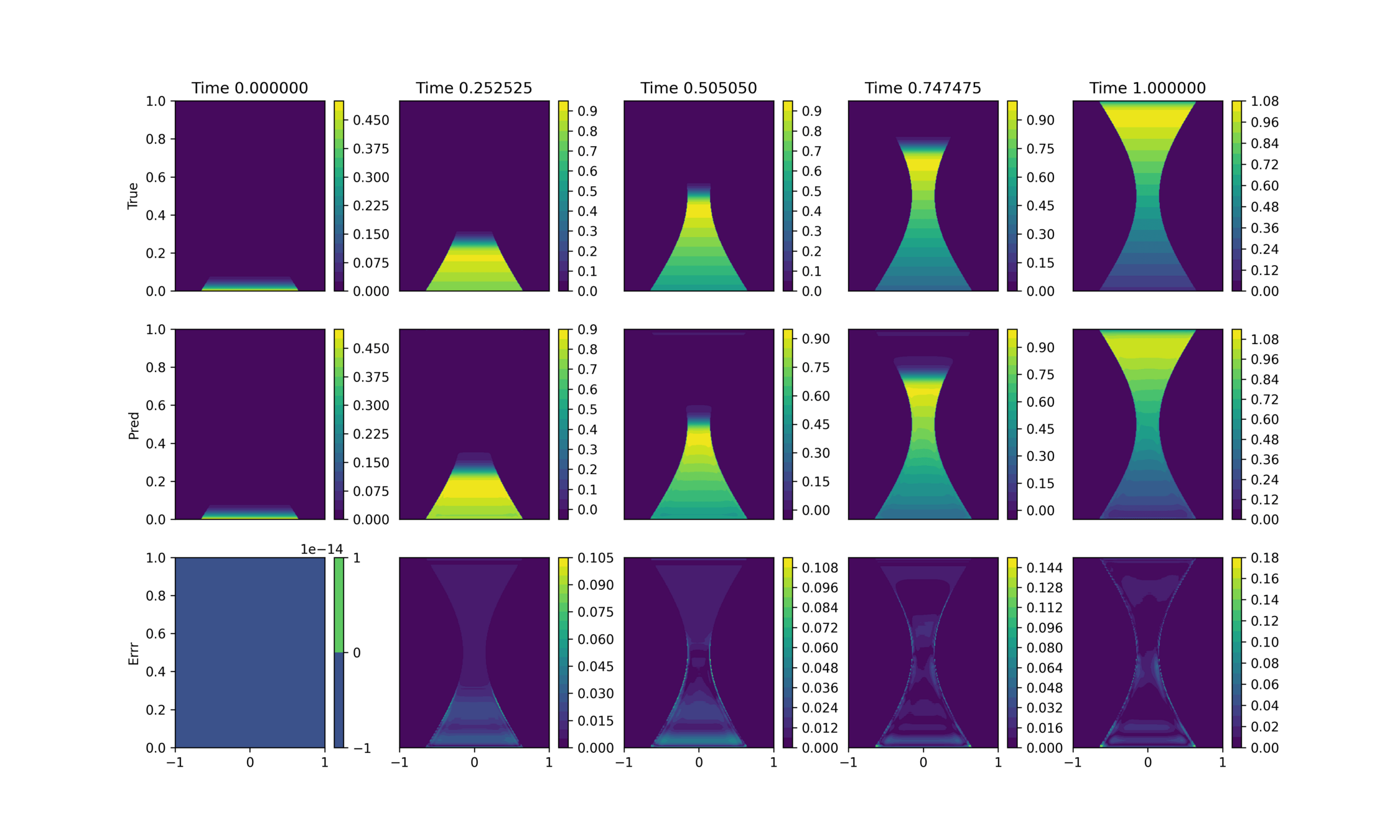
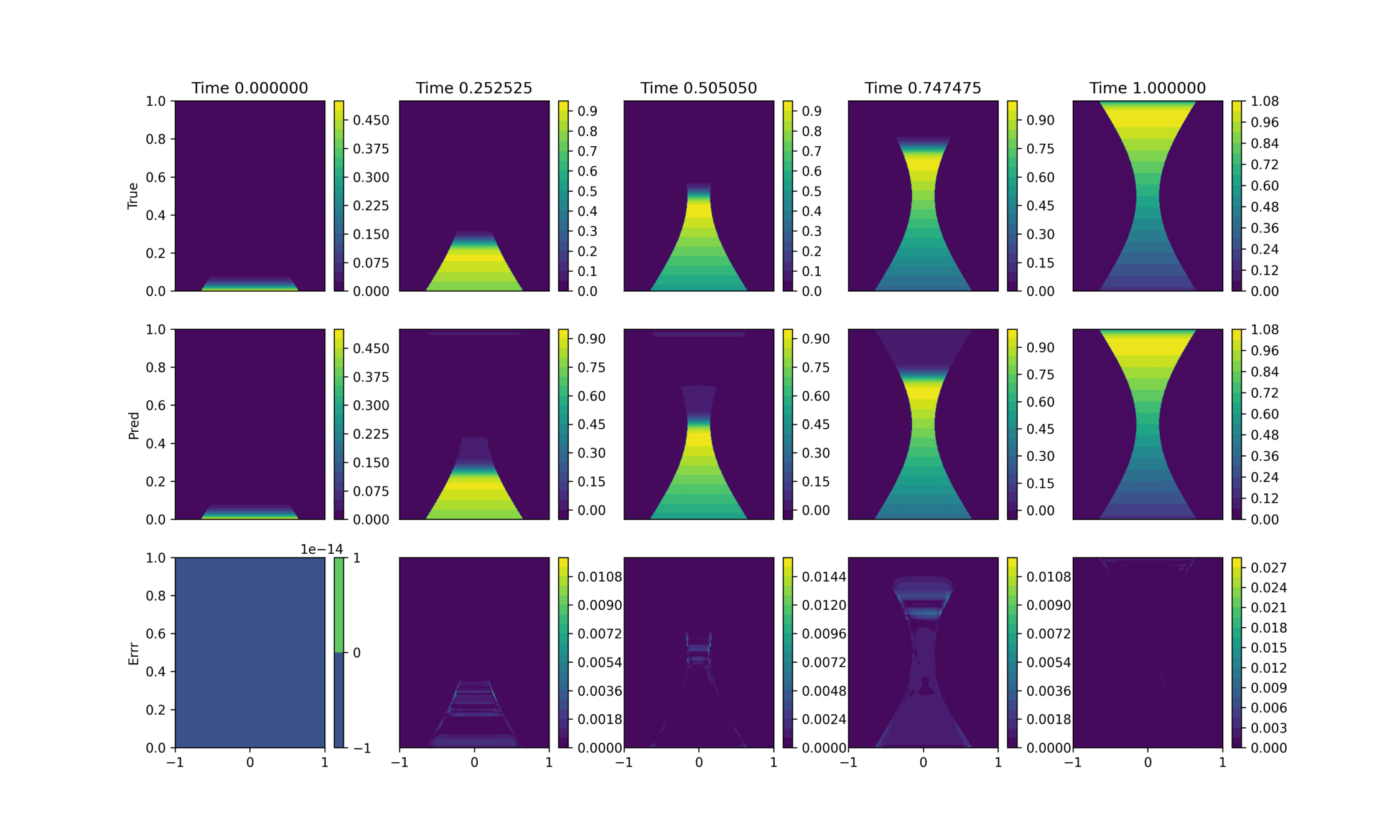
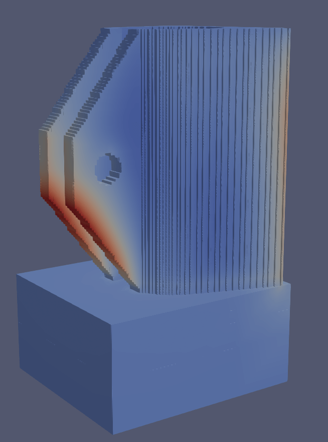
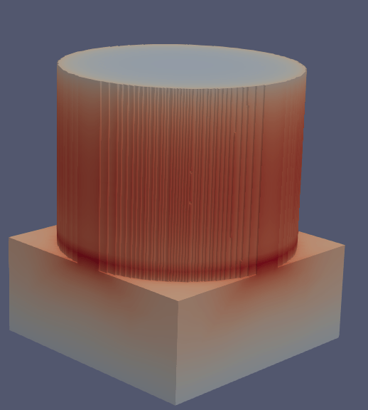
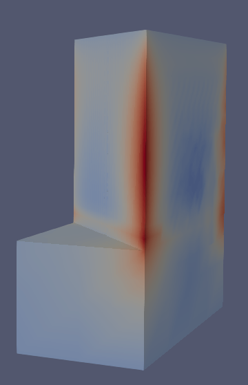
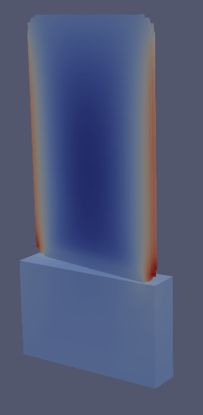
LPBF process simulation with Autodesk NetFabb
True
Prediction
Abs Error
Training on next-step prediction problem
Inference with auto-regressive rollout
Still seeing significant errors during rollout
Errors localized to the interface but much smaller
temperature_data = get_data()

temperatures = []
temperatures.append(temperature_data[0])

for time in 0:T # loop over time-steps
	curr_temp = temperatures[-1]
    next_temp = CNN(curr_temp, time, X, Z)
    temperatures.append(next_temp)
endPreviously funded projects (2023)
True
Prediction
Abs Error
Training on next-step prediction problem
Inference with auto-regressive rollout
Still seeing significant errors during rollout
Errors localized to the interface but much smaller
temperature_data = get_data()

temperatures = []
temperatures.append(temperature_data[0])

for time in 0:T # loop over time-steps
	curr_temp = temperatures[-1]
    next_temp = CNN(curr_temp, time, X, Z)
    temperatures.append(next_temp)
endNetFabb 3D Dataset (final time)
NetFabb 3D Dataset (time series)
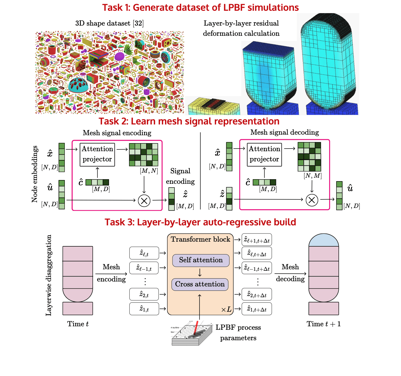
PMFI Proposal 2025
Modeling dynamical deformation in LPBF with neural network surrogates
Modeling dynamical deformation in LPBF with neural network surrogates
PROJECT STATUS
NetFabb 3D Dataset (time series)
Modeling dynamical deformation in LPBF with neural network surrogates
PROJECT STATUS
NetFabb 3D Dataset (time series)
Modeling dynamical deformation in LPBF with neural surrogates
Subgraph
extraction
interpolation
Neural network prediction
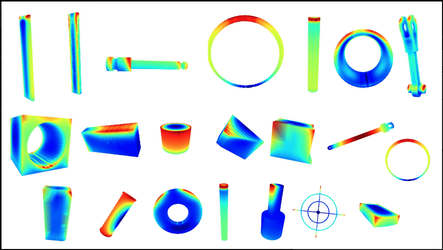
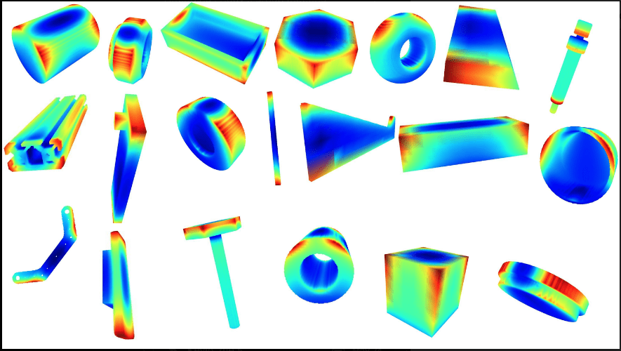
Model is trained on 30 shapes. These are results from the test set
Baseline
Our approach
-0.05
0.43
0.28
0.69
0.56
0.80
-3.55
-0.20
Auto-regressive predictions at the final time-step
Baseline
Our approach
0.97
0.99
0.99
0.99
0.97
0.99
0.96
0.99
Predictions given ground truth at final time-step
test01
test09
test06
test00
Observations
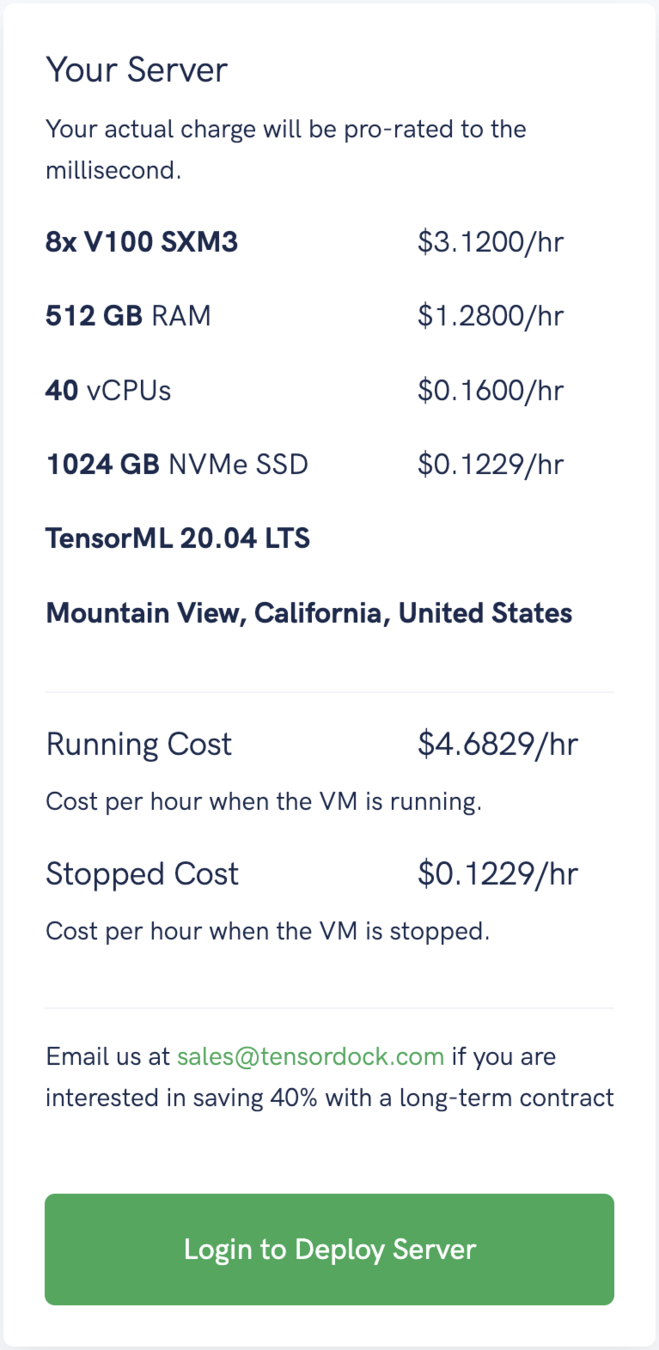
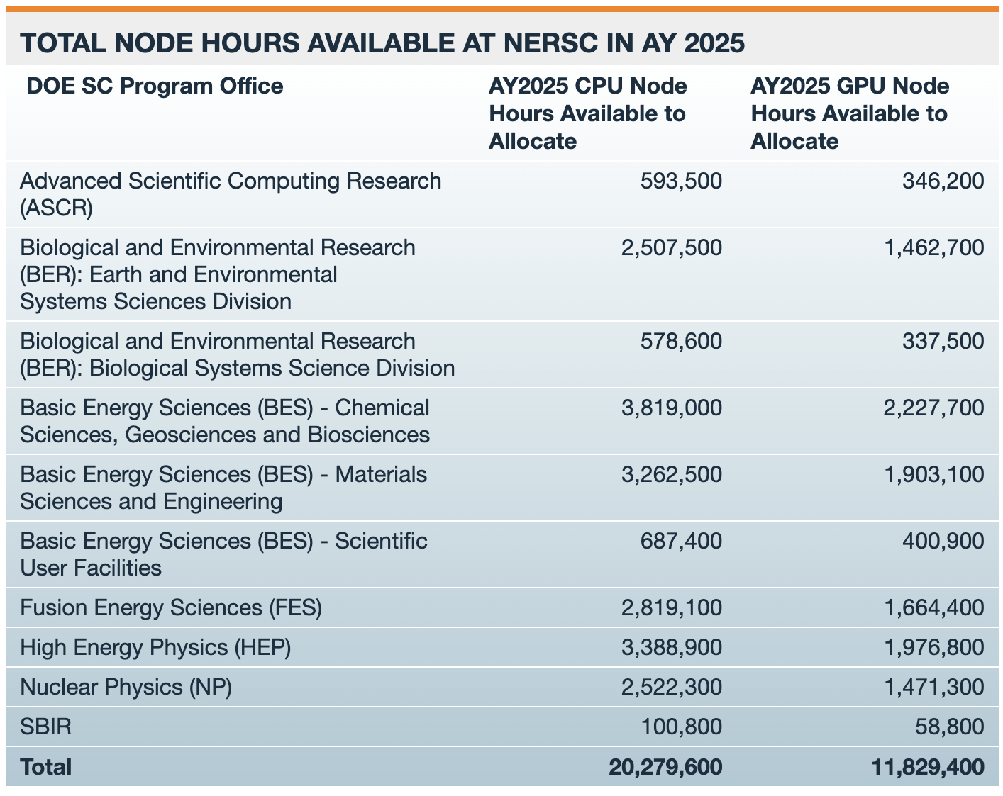
Blockers: Limited GPU compute available
Same configuration as PSC Bridges
Modeling dynamical deformation in LPBF with neural network surrogates
PROJECT STATUS
Spatial Discretization
Temporal Discretization
Graph Neural Networks
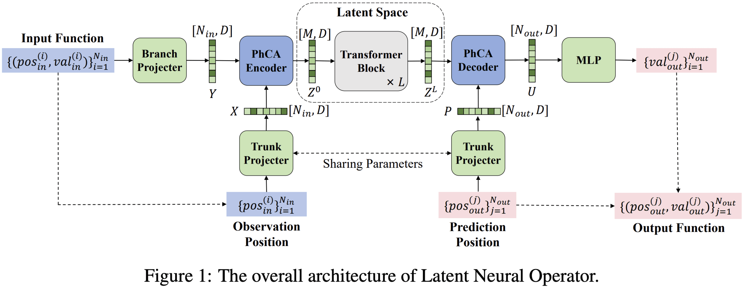
Transformer embedding representation
Neural implicits
Next-step prediction
LSTM or related architecutre
Transformer
next-step prediction
Modeling dynamical deformation in LPBF with neural network surrogates
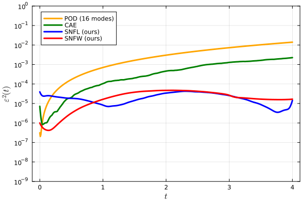
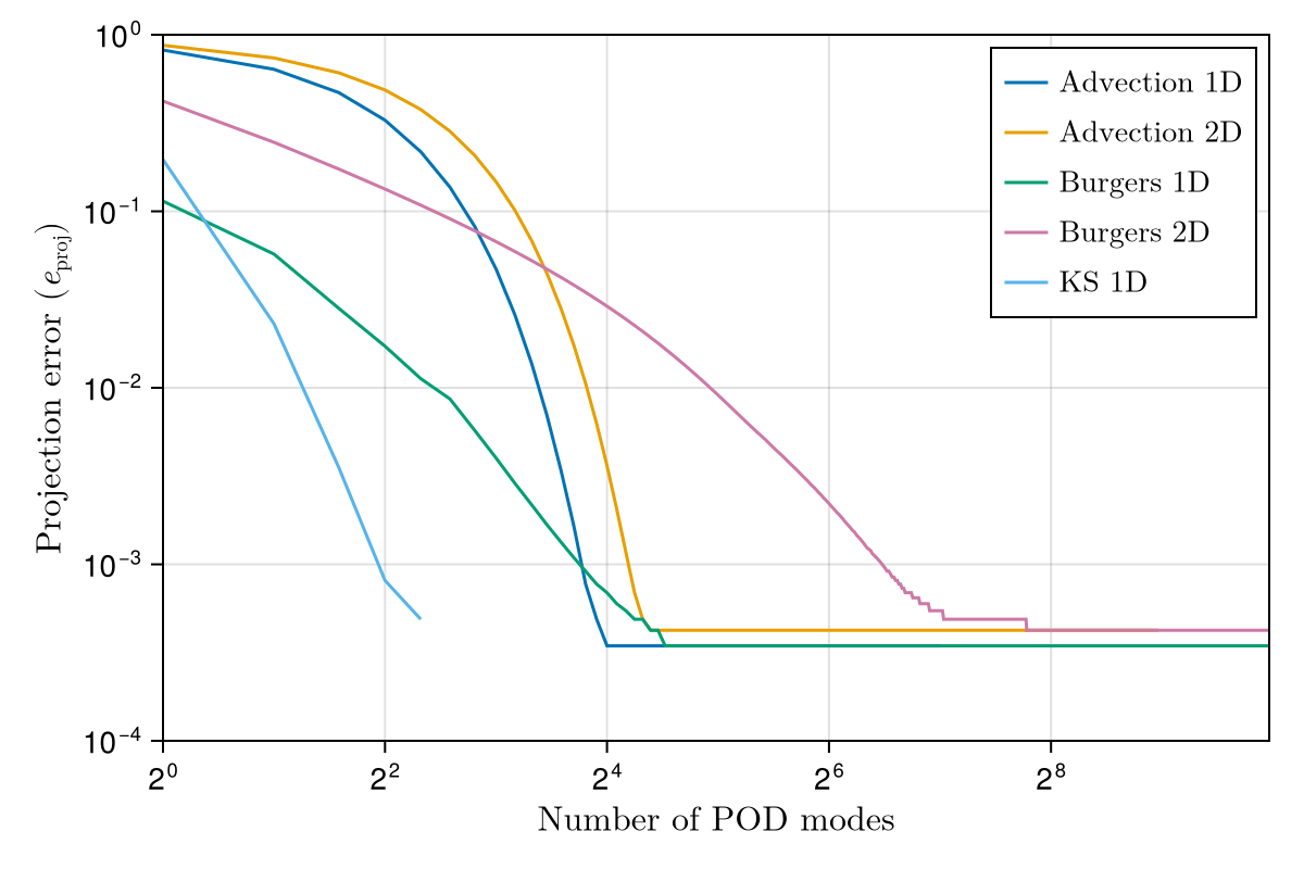
SNF-ROM paper revisions for Journal of Computational Physics
SNF-ROM paper revisions for Journal of Computational Physics
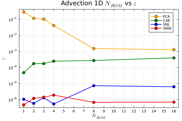
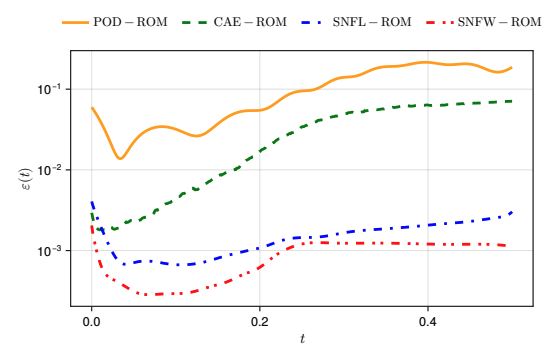
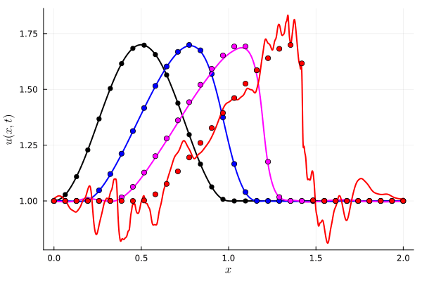
1D Advection
Slow energy decay in POD modes
Modeling dynamical deformation in LPBF with neural network surrogates
PROJECT STATUS
Spatial Discretization
Temporal Discretization
Graph Neural Networks
Transformer embedding representation
Neural implicits
Next-step prediction
LSTM or related architecutre
Transformer
next-step prediction
Modeling dynamical deformation in LPBF with neural network surrogates
Modeling dynamical deformation in LPBF with neural surrogates
Subgraph
extraction
interpolation
Neural network prediction
CAD = get_CAD_geometry()
displacement = []

for l in 1:num_layers(CAD) # loop over layers

	# slice geometries
	next_cad_layer = CAD[l]
    prev_layer_disp = displacement[1:l-1]

    # our model
    next_layer_disp = NN(next_cad_layer, prev_layer_disp)

	# update Geometry
	displacement.append(next_layer_disp)
end

asbuilt_geometry = CAD + displacement
asbuilt_geometry.visualize()Model trained on 30 shapes. These are results from the test set
Baseline
Our approach
-0.05
0.43
0.28
0.69
0.56
0.80
-3.55
-0.20
Auto-regressive predictions at the final time-step
Baseline
Our approach
0.97
0.99
0.99
0.99
0.97
0.99
0.96
0.99
Predictions given ground truth
Training is successful!
Auto-regressive evaluation yields mixed results
Overall improvement over baseline
Success
Failure
Modeling dynamical deformation in LPBF with neural network surrogates
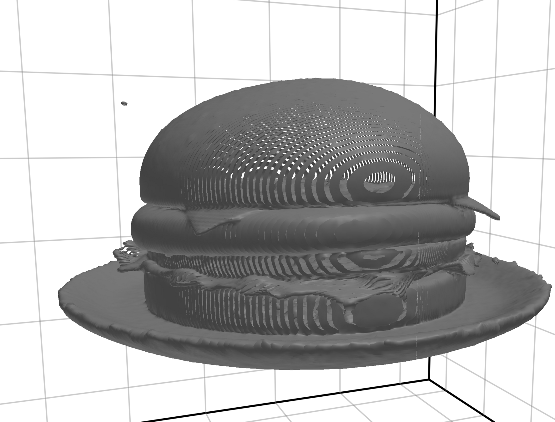
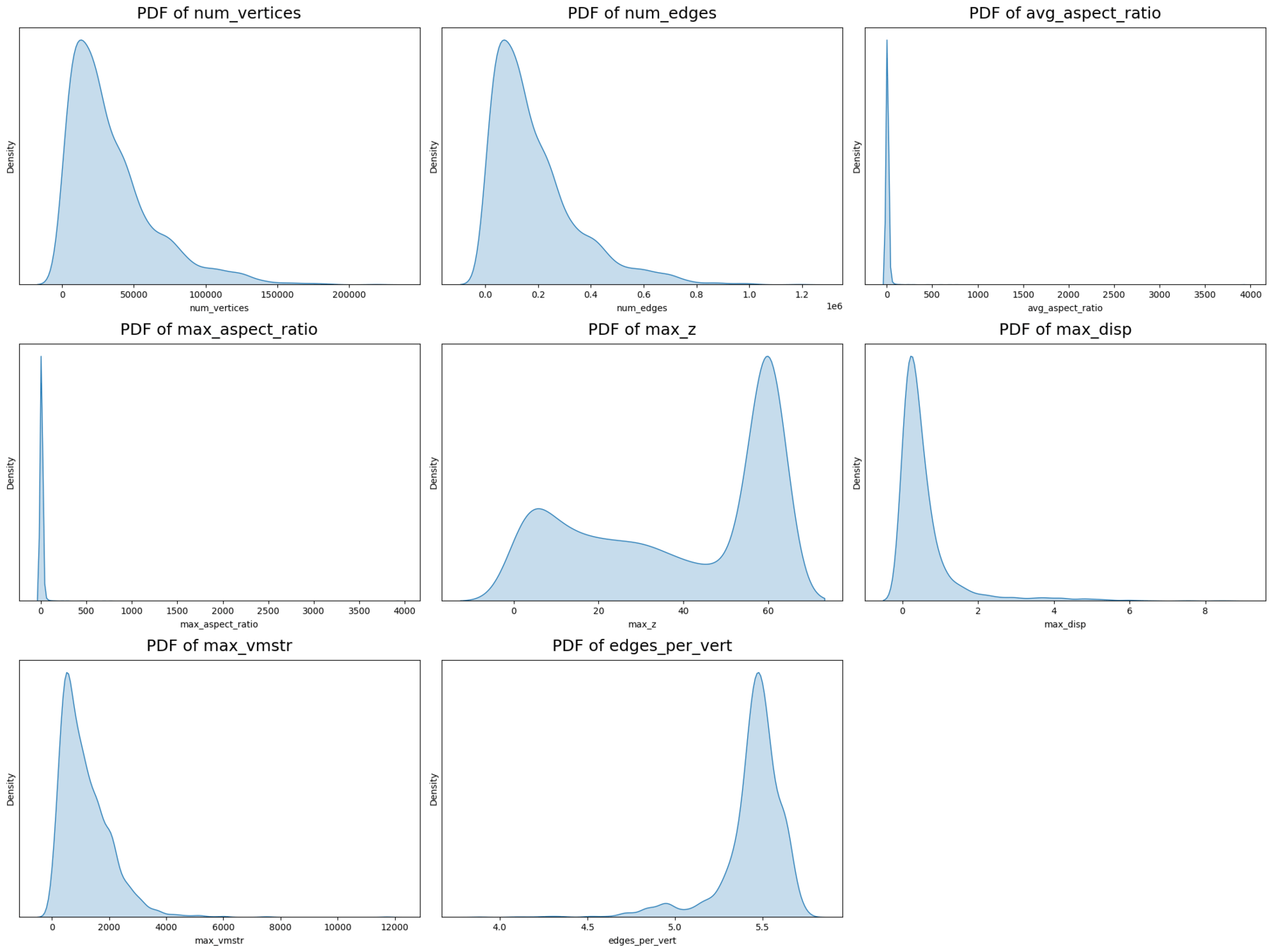
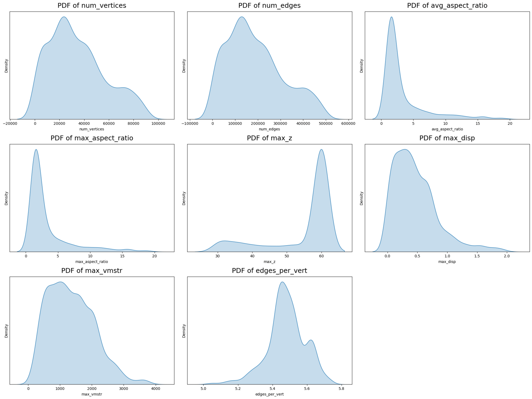
Original dataset
Filtered dataset
Large meshes
Thin shapes
Large meshes
Original dataset
Filtered dataset
Thin features
Too few layers
Bad simulator
Original dataset
Filtered dataset
Bad simulator
Thin shapes
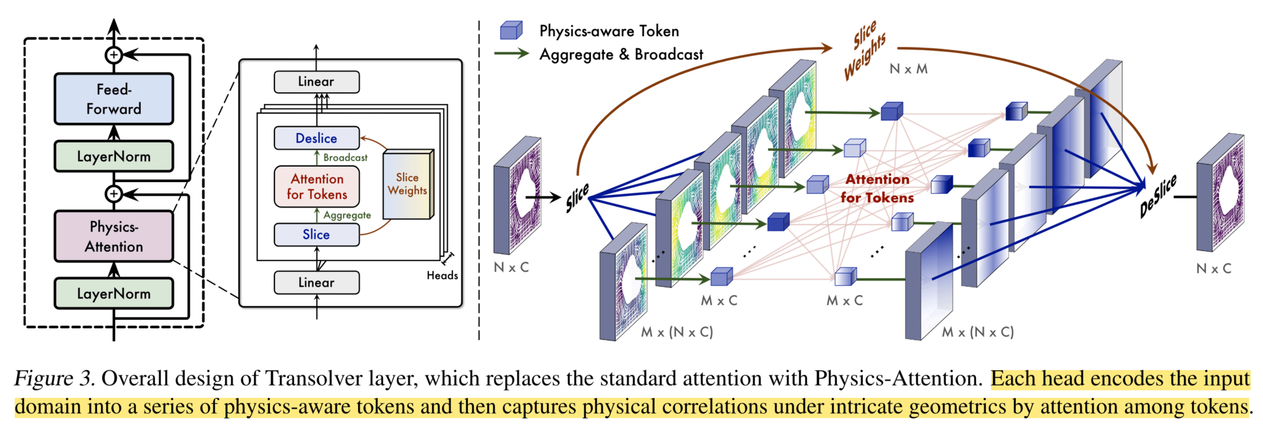
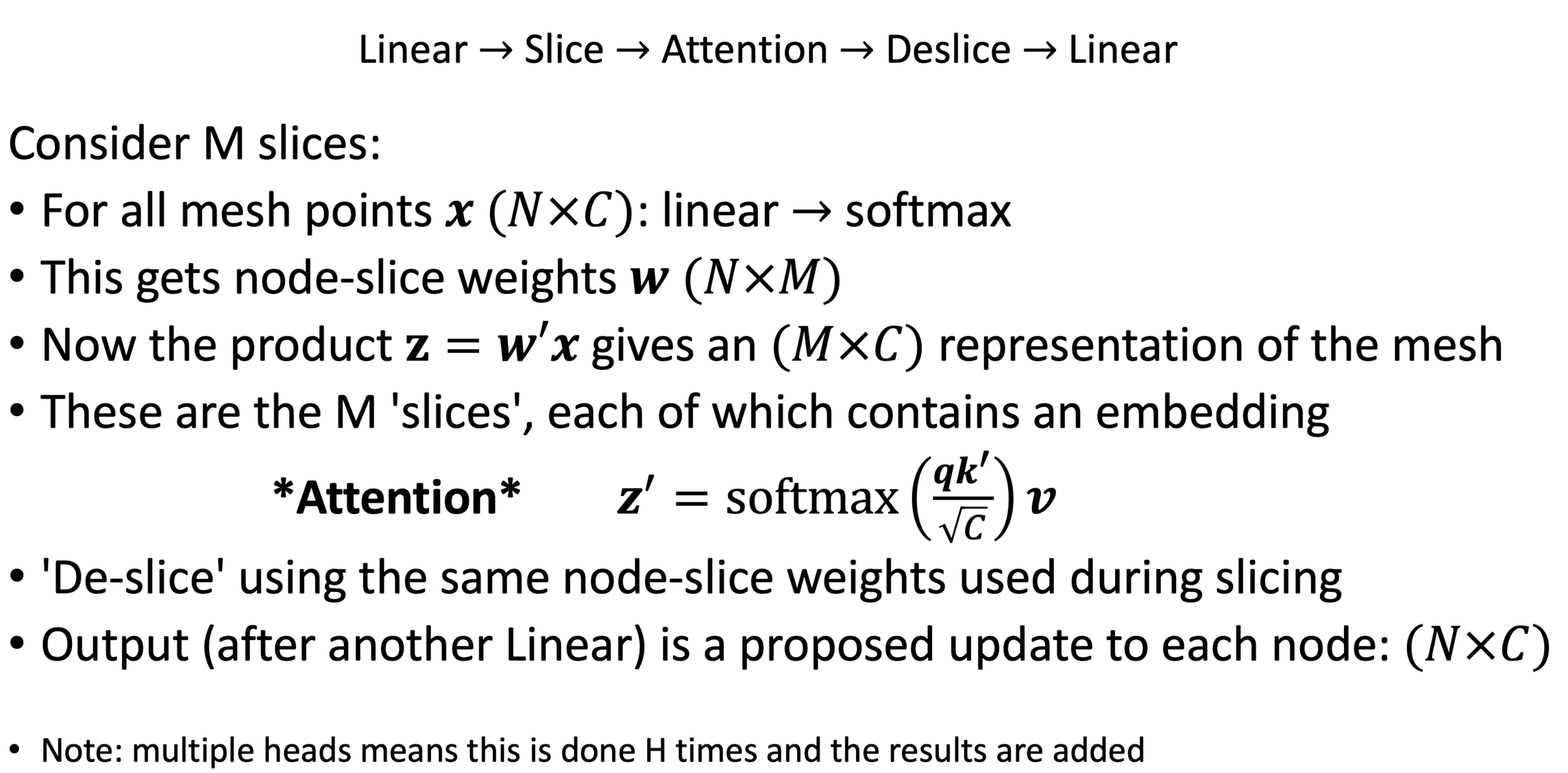
Transolver
Mesh Graph Net
Modeling dynamical deformation in LPBF with neural network surrogates
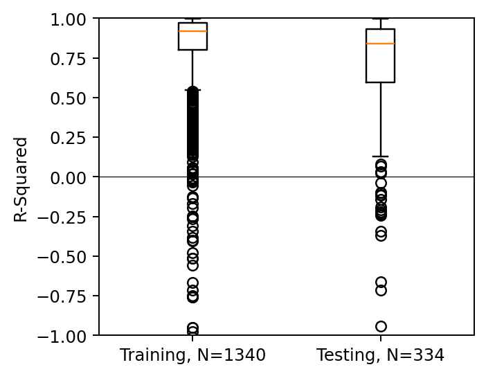
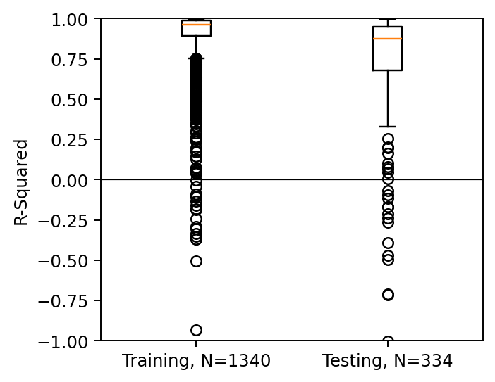
Vanilla MeshGNN
Vanilla Transolver
Training (N=191)
Test set (N=47)
Transolver + Pipeline
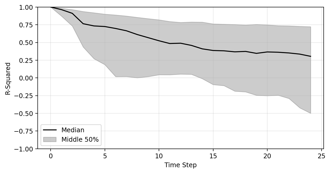
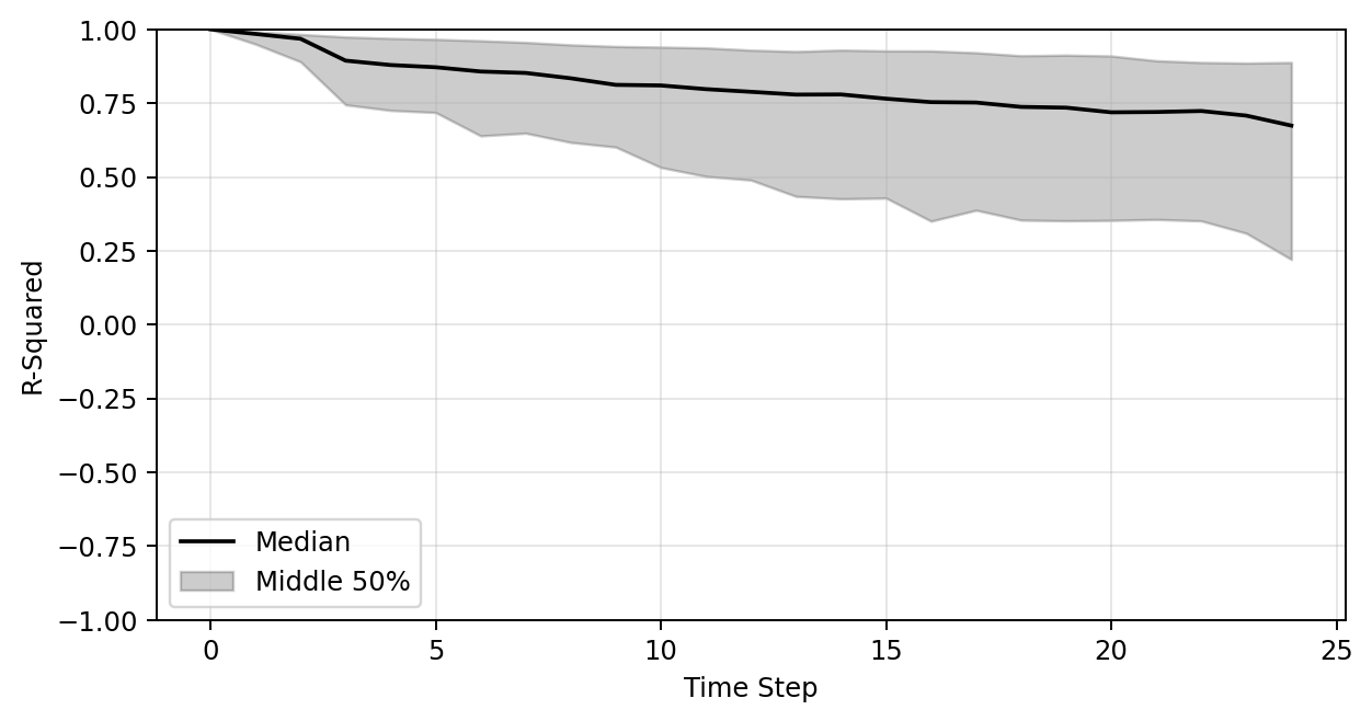
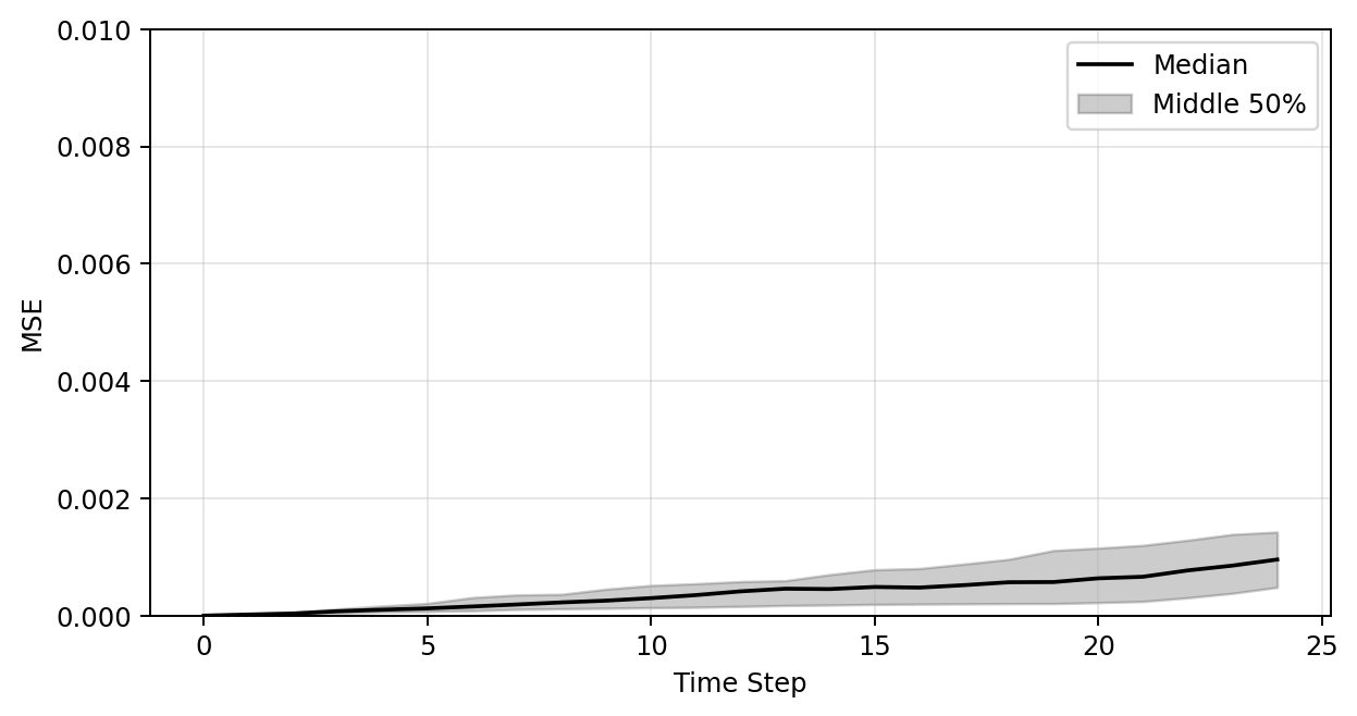
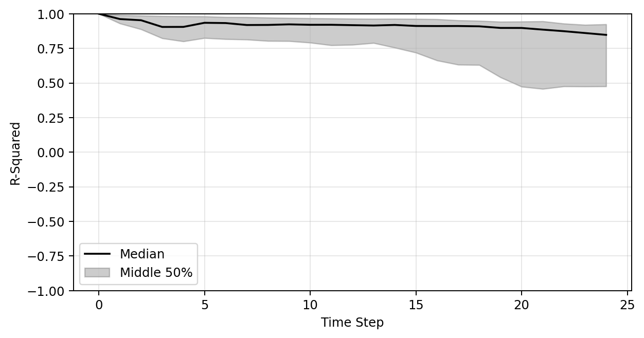
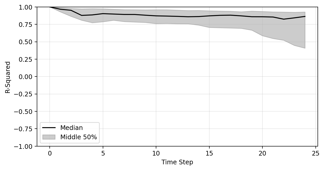
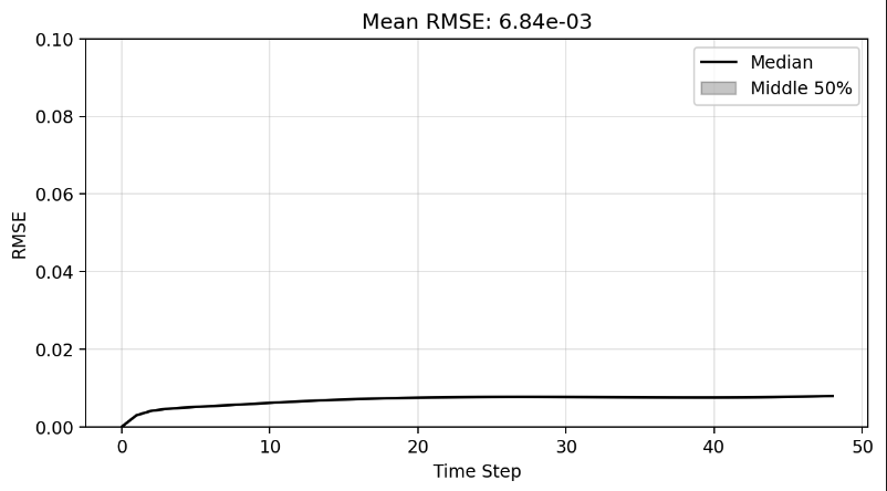
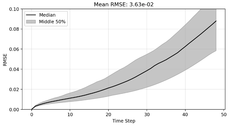
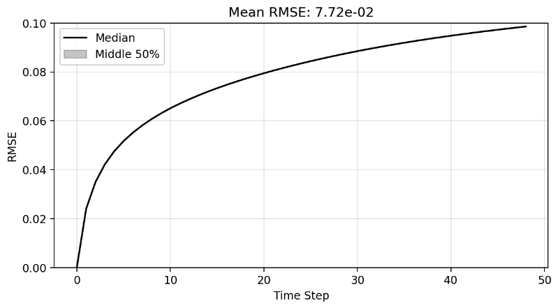
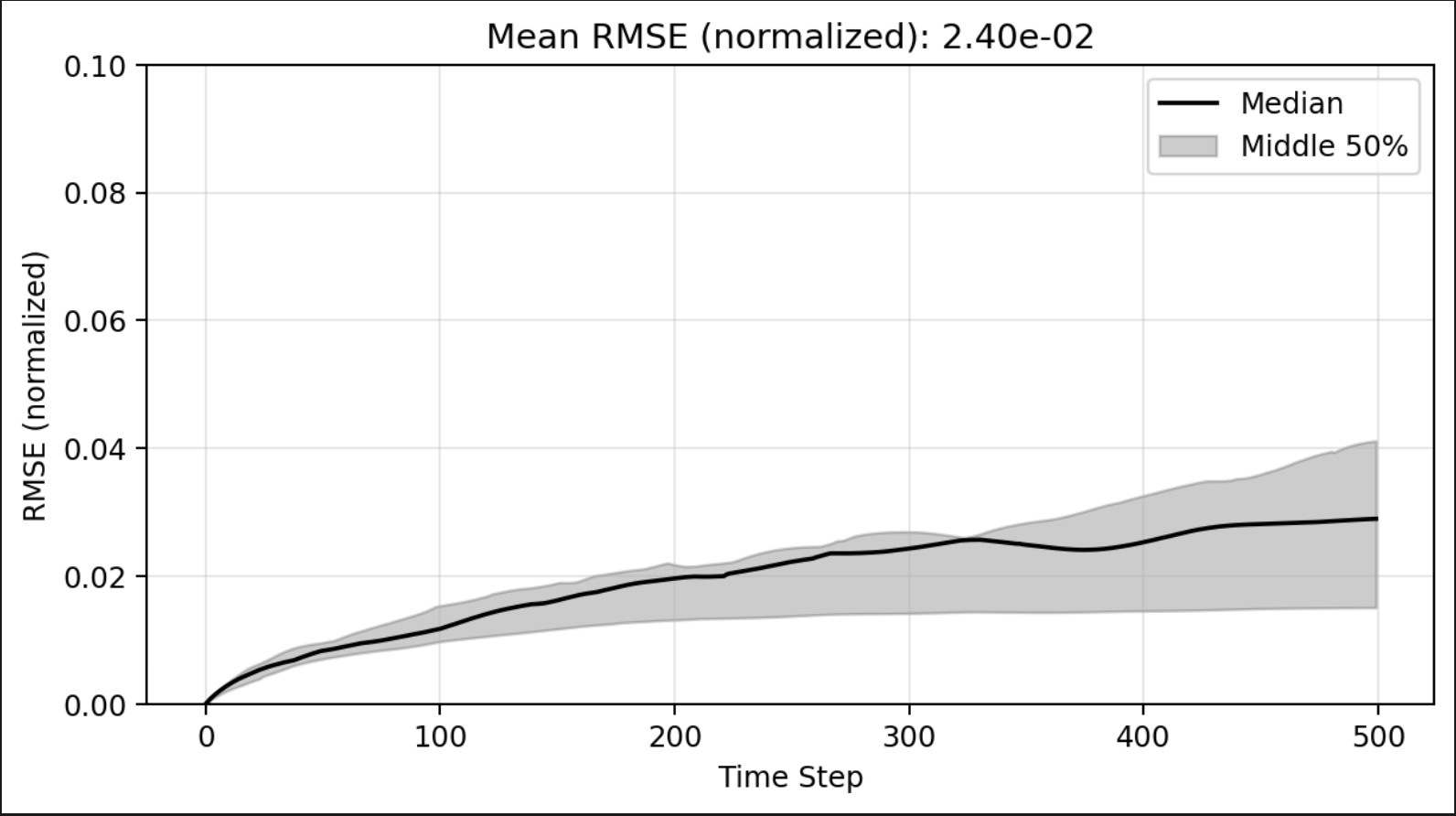
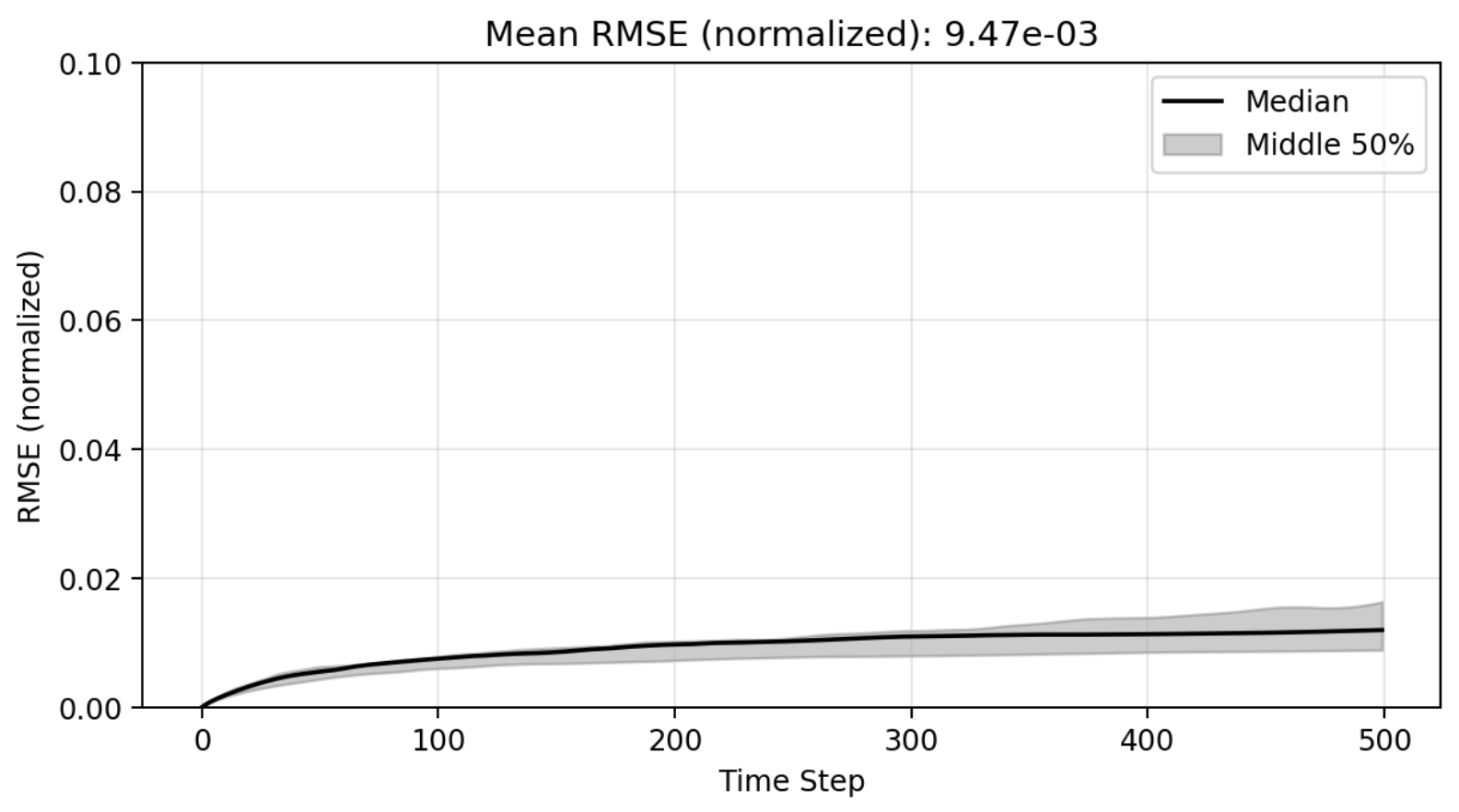
Plot of R-sqaure accuracy vs time-step during auto-regressive rollout
Large variance
Improved stability
Poor generalization so far
| Vanilla MeshGNN | Vanilla transolver | Transolver + Pipeline | |
|---|---|---|---|
| Training set (191 shapes) | 0.27 | 0.45 | 0.65 |
| Test set (47 shapes) | 0.24 | 0.48 | 0.49 |
R-sqaure accuracy at the final time-step
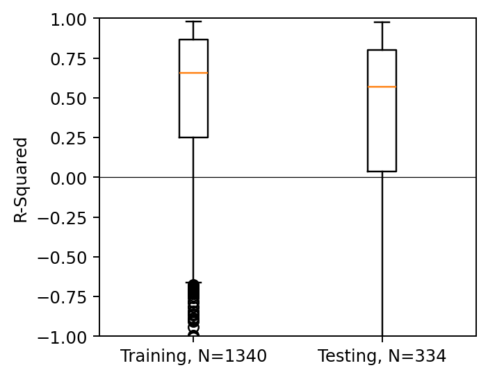
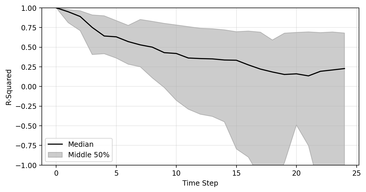
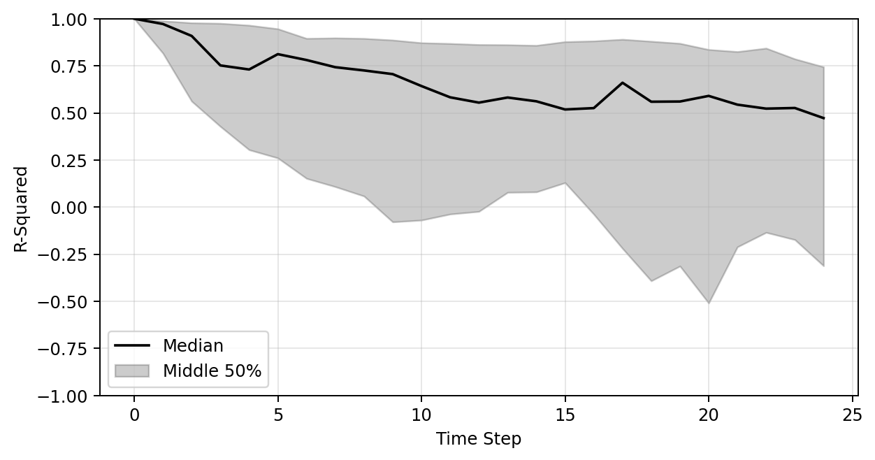
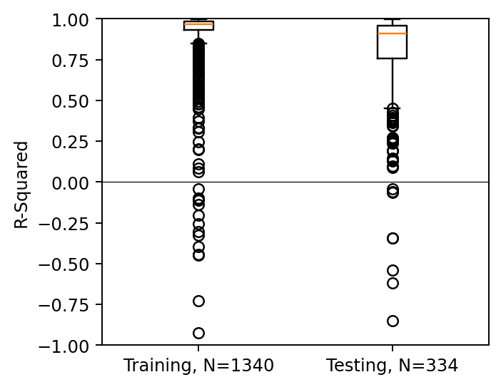
FROM YESTERDAY
Vanilla MeshGNN
Vanilla Transolver
Training (N=191)
Test set (N=47)
Transolver + Pipeline
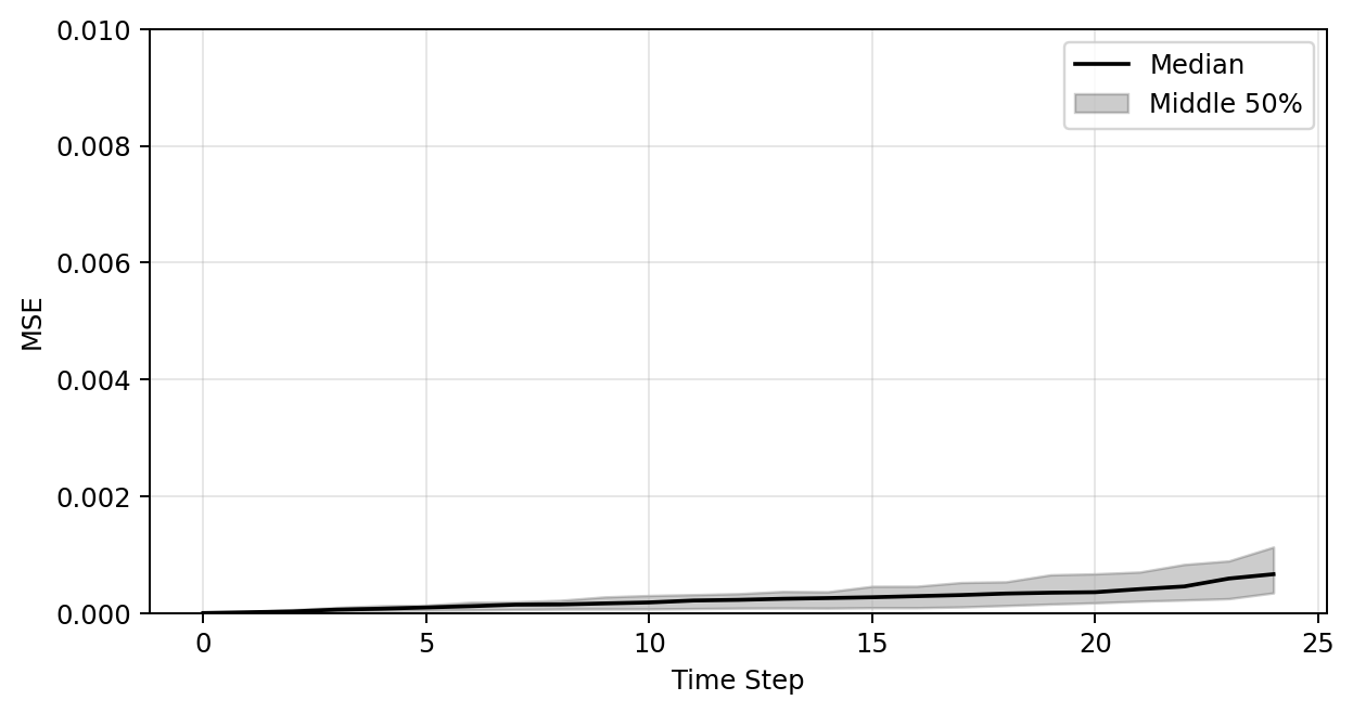
Plot of R-sqaure accuracy vs time-step during auto-regressive rollout
Large variance
Improved stability
Better generalization
| Vanilla MeshGNN | Vanilla transolver | Transolver + Pipeline | |
|---|---|---|---|
| Training set (191 shapes) | 0.27 | 0.45 | 0.68 |
| Test set (47 shapes) | 0.24 | 0.48 | 0.65 |
Median R-sqaure accuracy at the final time-step
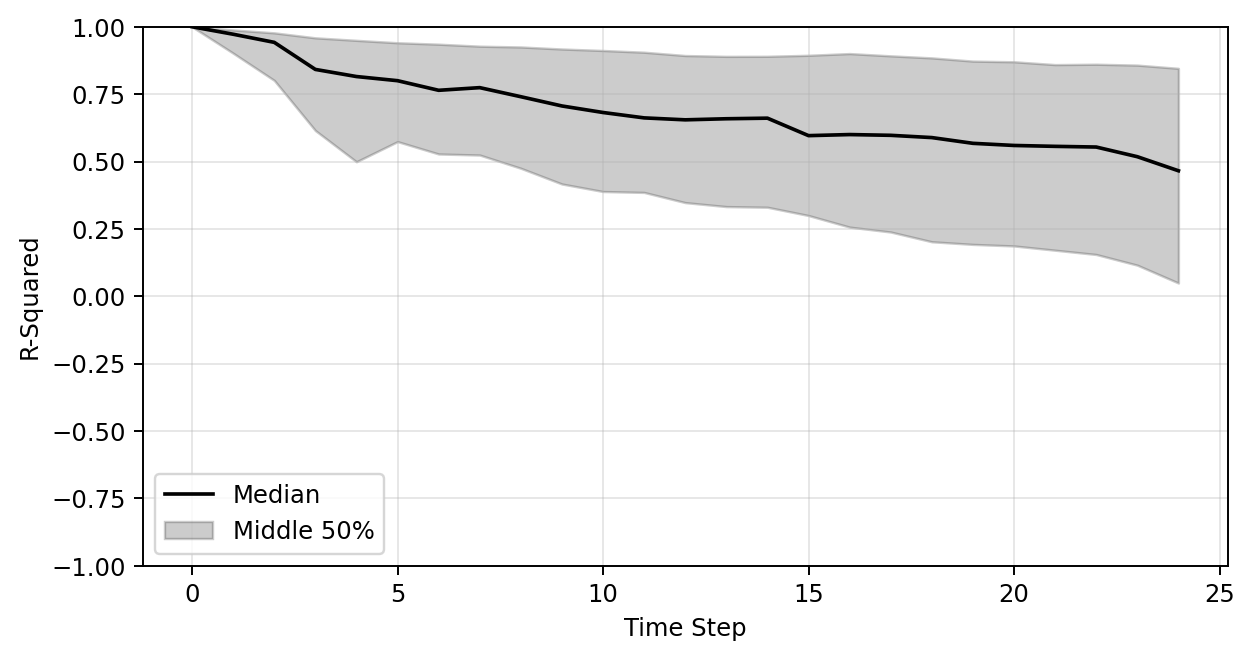
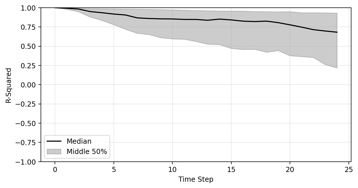
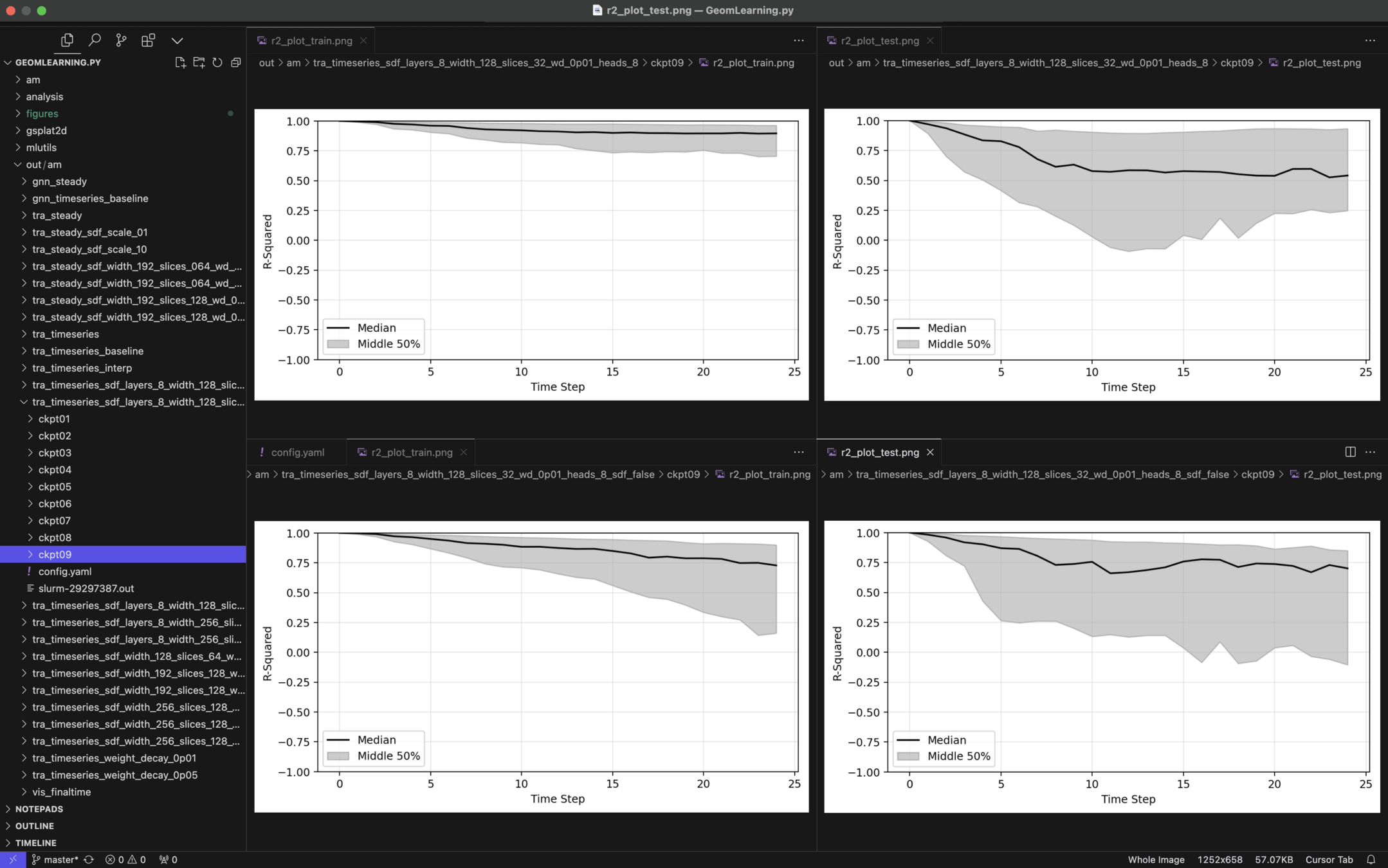
Vanilla Transolver
Vanilla MeshGraphNet
Transolver + SDF Feature
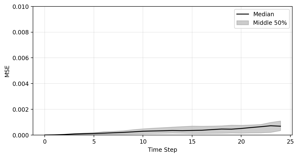
Plots of R-sqaure accuracy
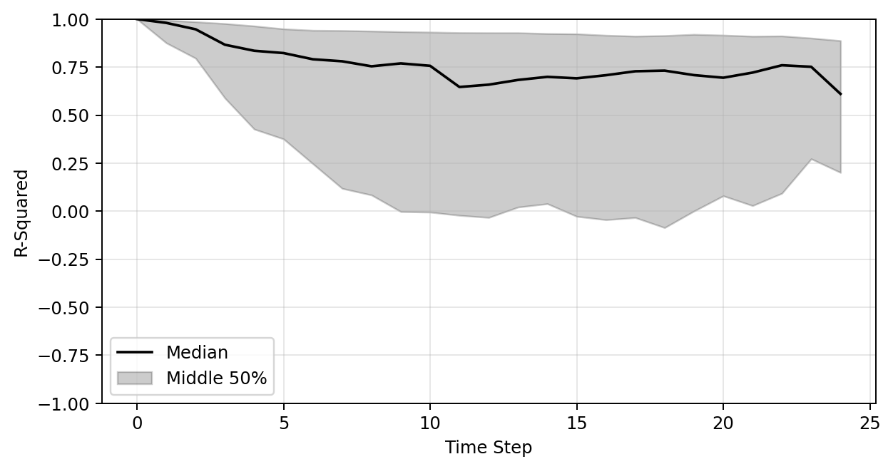
Modeling dynamical deformation in LPBF with neural network surrogates
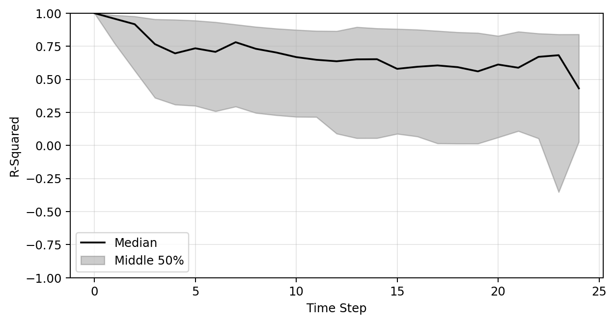
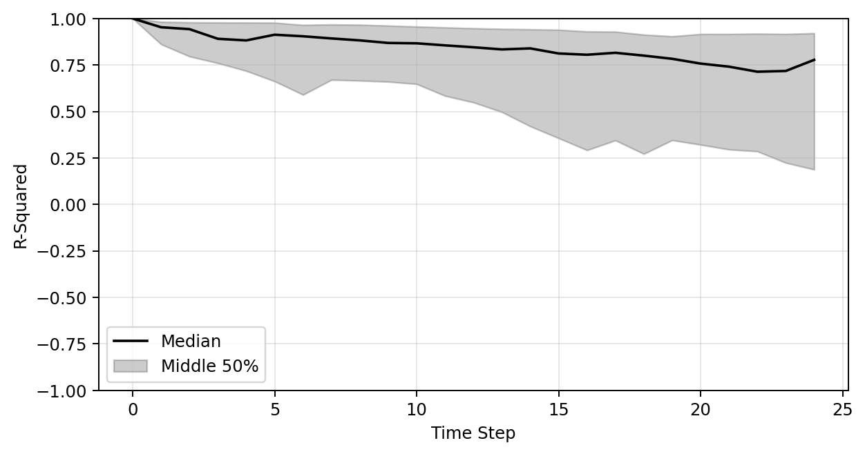
Transolver
MeshGraphNet
Transolver + SDF Feature + longer training
Plots of R-sqaure accuracy
Modeling dynamical deformation in LPBF with neural network surrogates
Modeling dynamical deformation in LPBF with neural network surrogates
Vanilla Transolver
+ Pipeline
Cluster Attention + AdaLN
+ Pipeline (OURS)
Cluster Attention + Q-Conditioning
+ Pipeline (OURS)
| Transolver + pipeline | Cluster Attention + AdaLN + Pipeline (OURS) | Cluster Attention + Q-Conditioning + Pipeline (OURS) | |
|---|---|---|---|
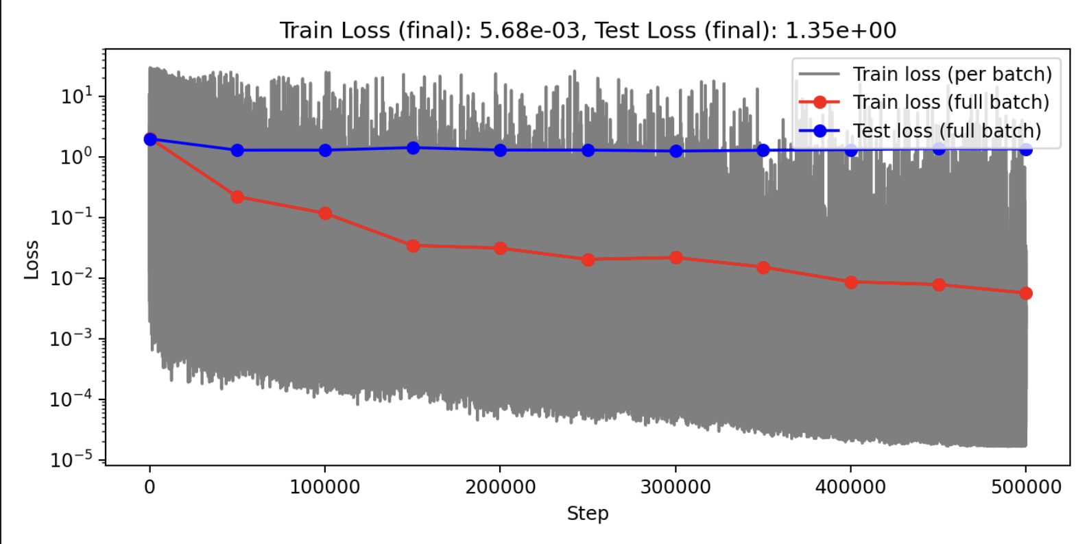
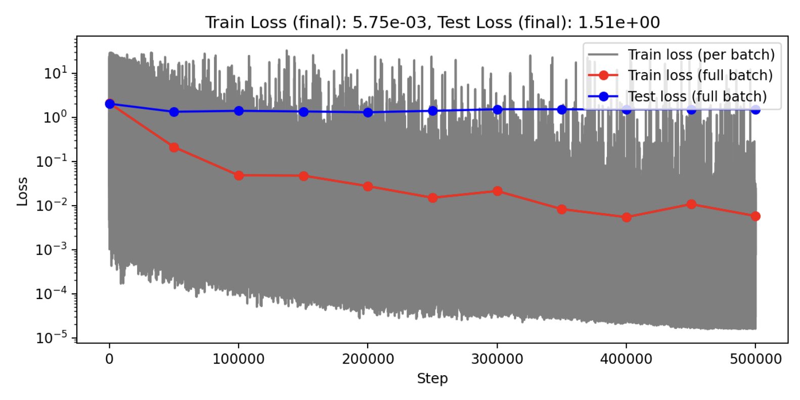
| MSE Loss | 7.38e-5 | 6.15e-5 | 4.99e-5 |
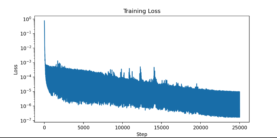
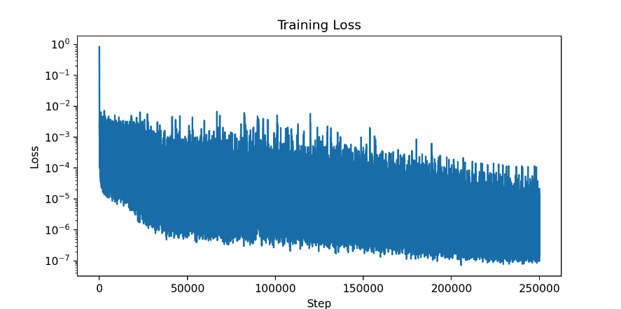
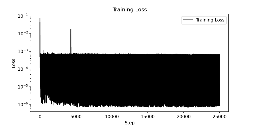
Training statistics
Advanced Robotics for Manufacturing (ARM) Institute
Modeling dynamical deformation in LPBF with neural network surrogates
Modeling dynamical deformation in LPBF with neural network surrogates
1 case
100 cases
Transolver
Transolver + AdaLN Conditioning
Transolver + Q-Conditioning
Allied Additive Manufacturing Interoperability (AAMI) Program
Modeling dynamical deformation in LPBF with neural network surrogates
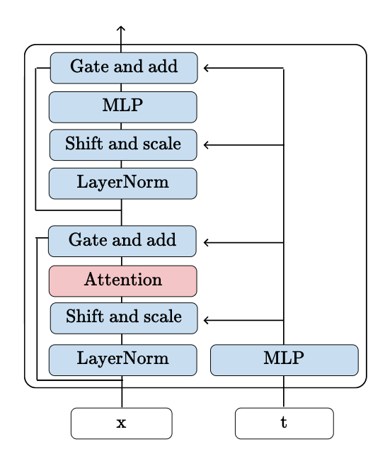
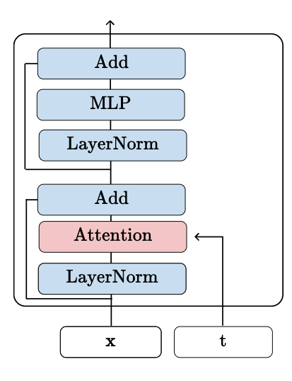
Adaptive LayerNorm Block
Q-Conditioning Block
Methods for time conditioning
Mesh Graph Net
Transolver
Transolver + AdaLN Conditioning
Transolver + AdaLN Conditioning
Transolver + AdaLN + Slice Attn
Transolver + Qcond + Slice Attn
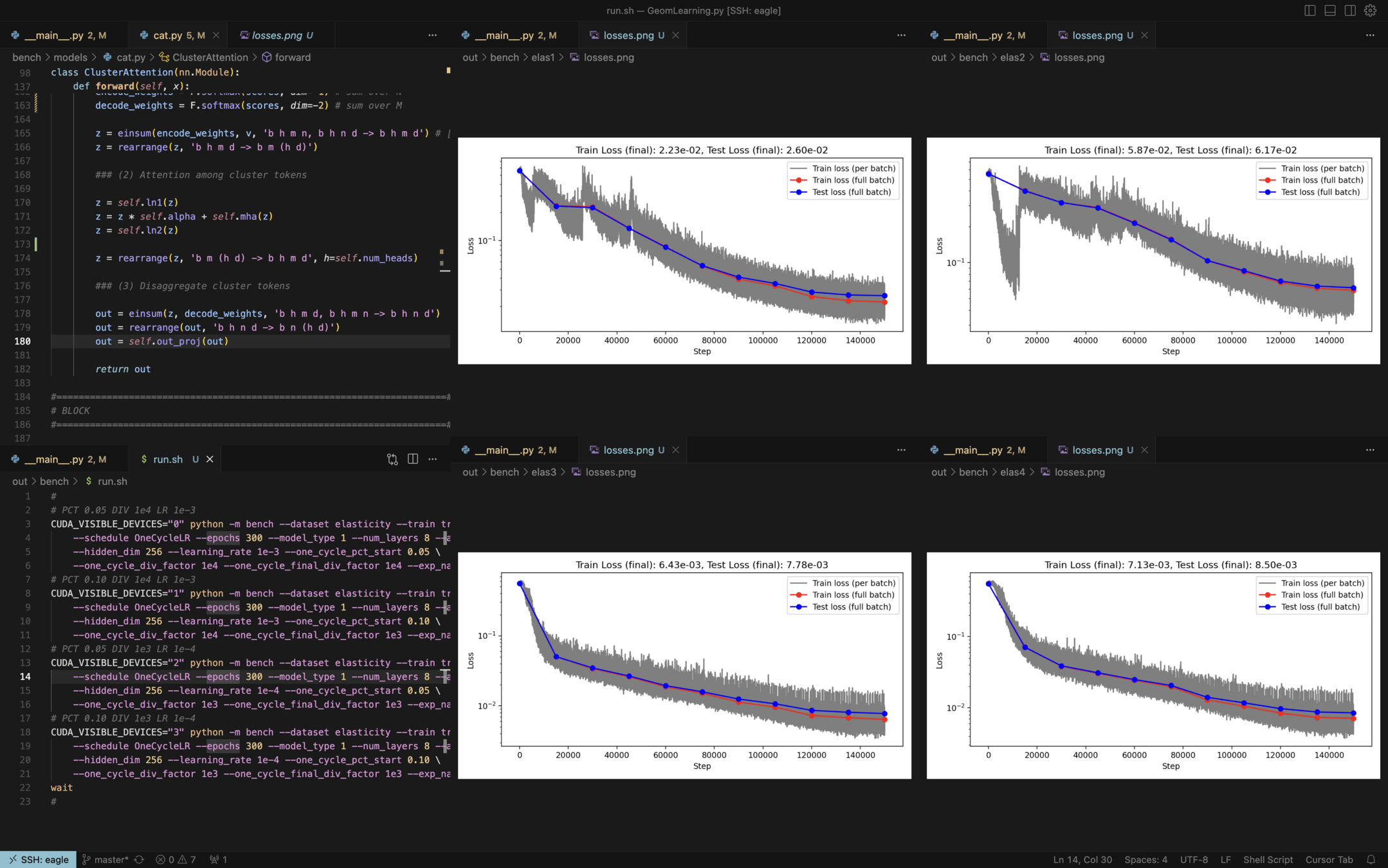
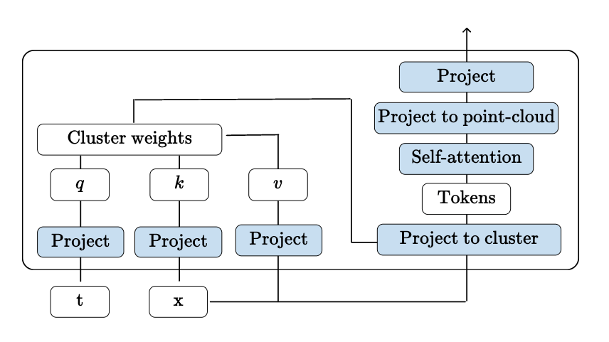
Cluster attention: stable point-cloud attention for learning physical fields
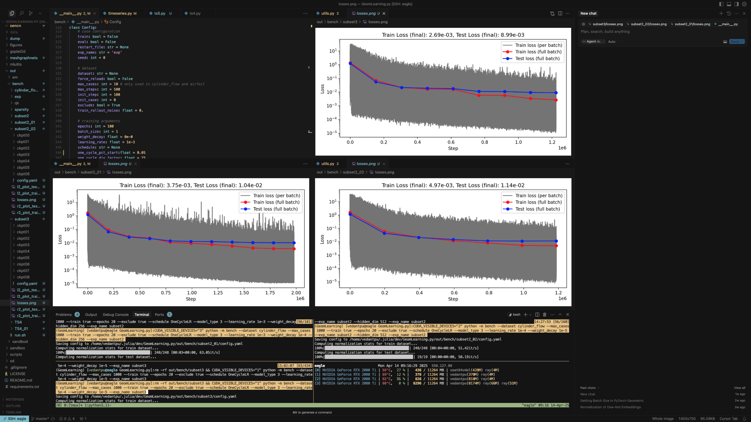
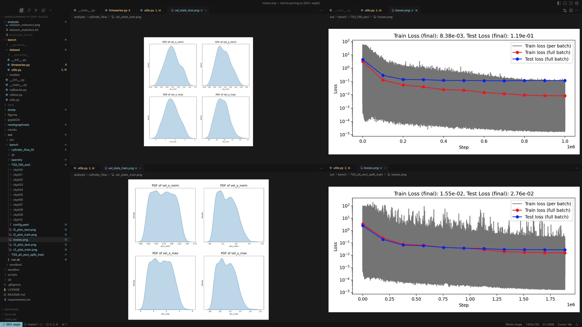
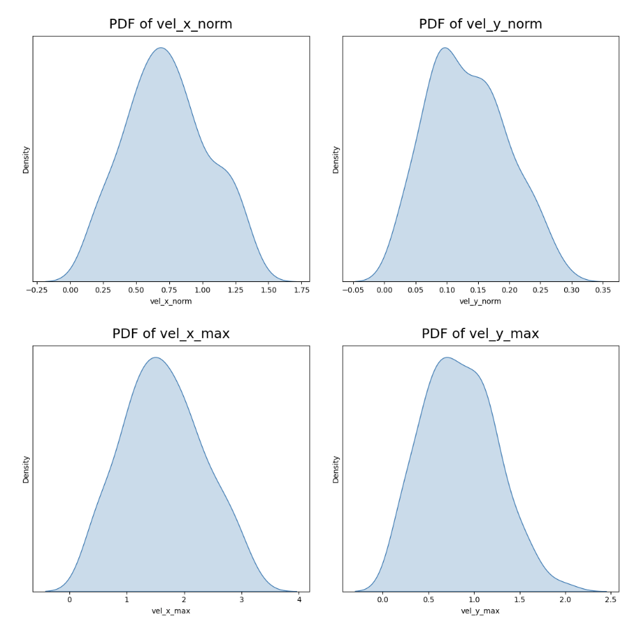
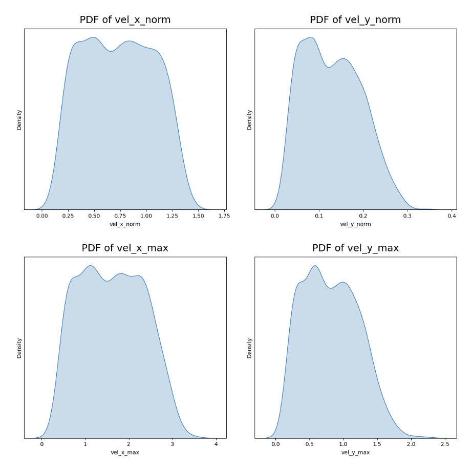
Train dataset stats (100 cases)
Test dataset stats (100 cases)
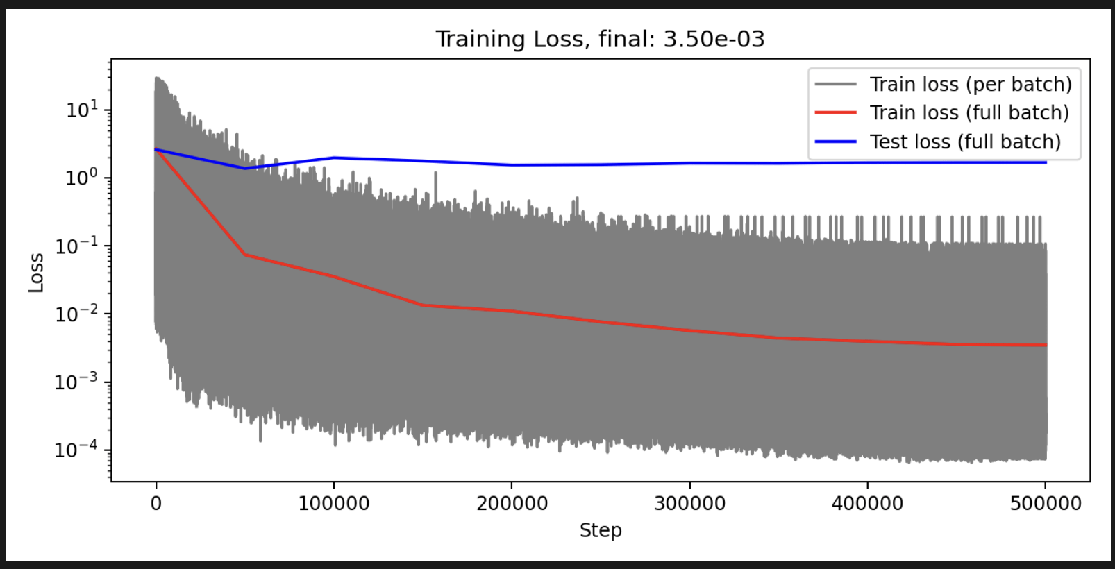
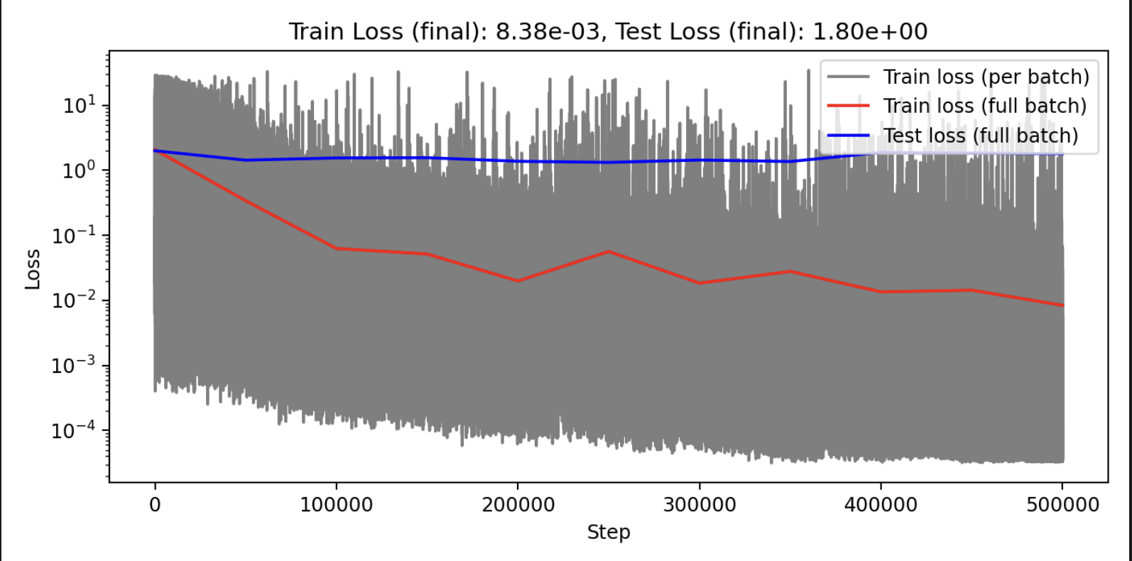
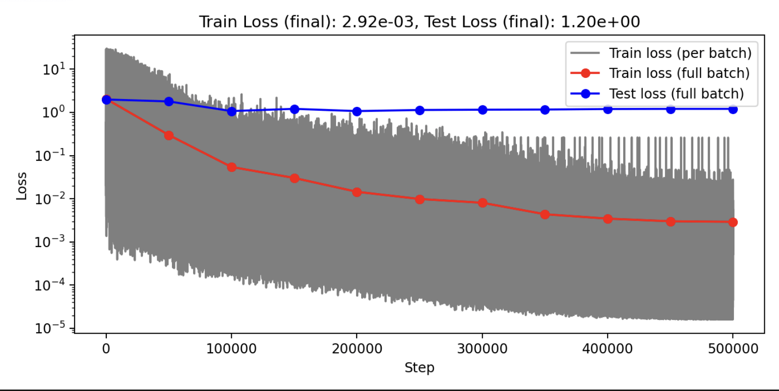
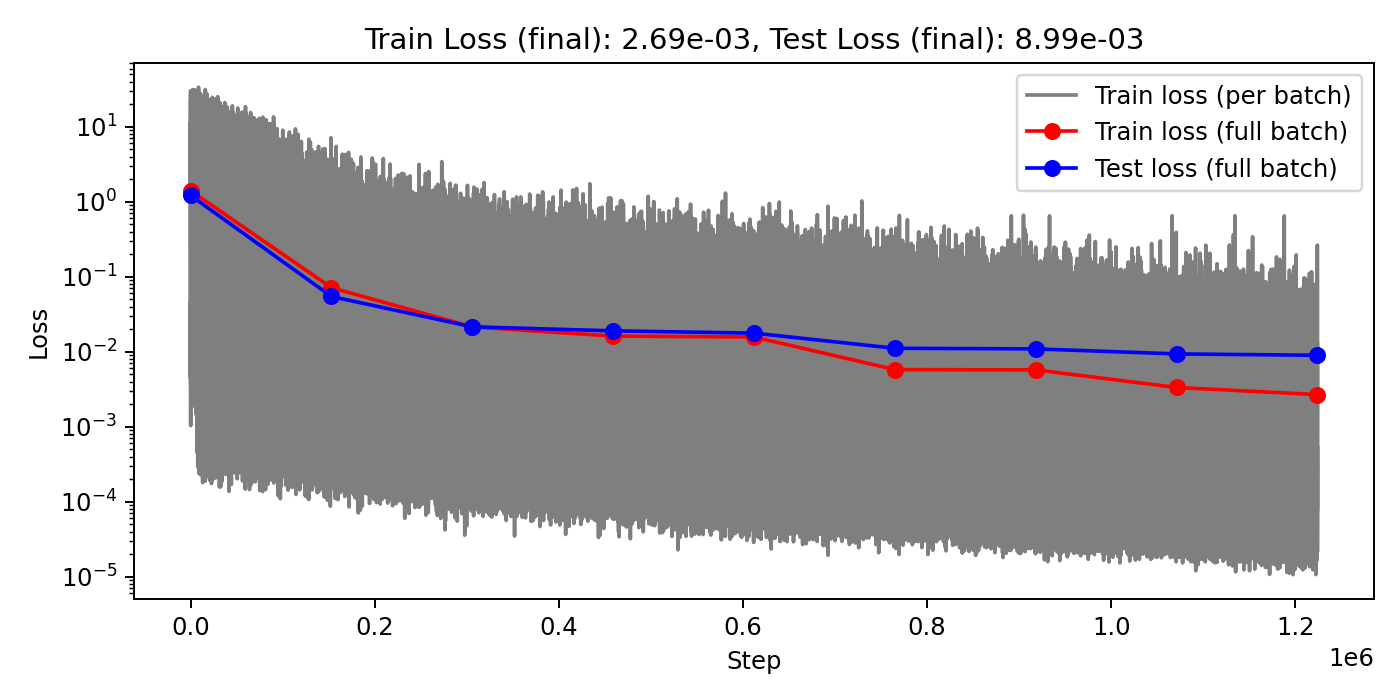
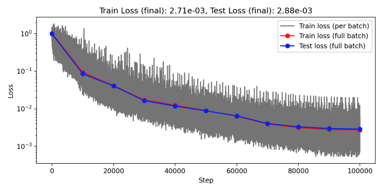
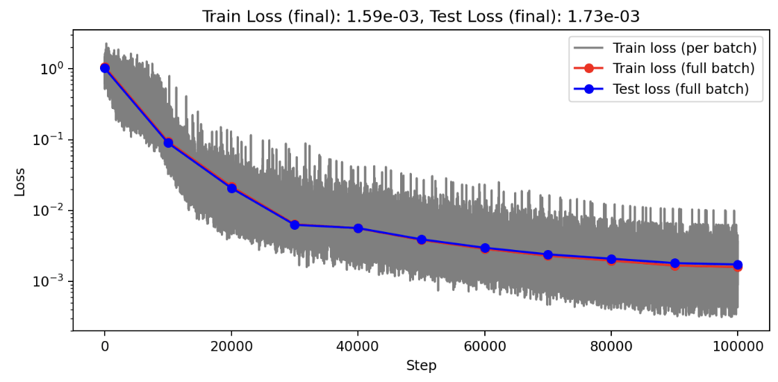
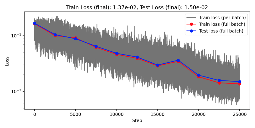
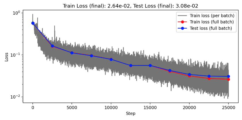
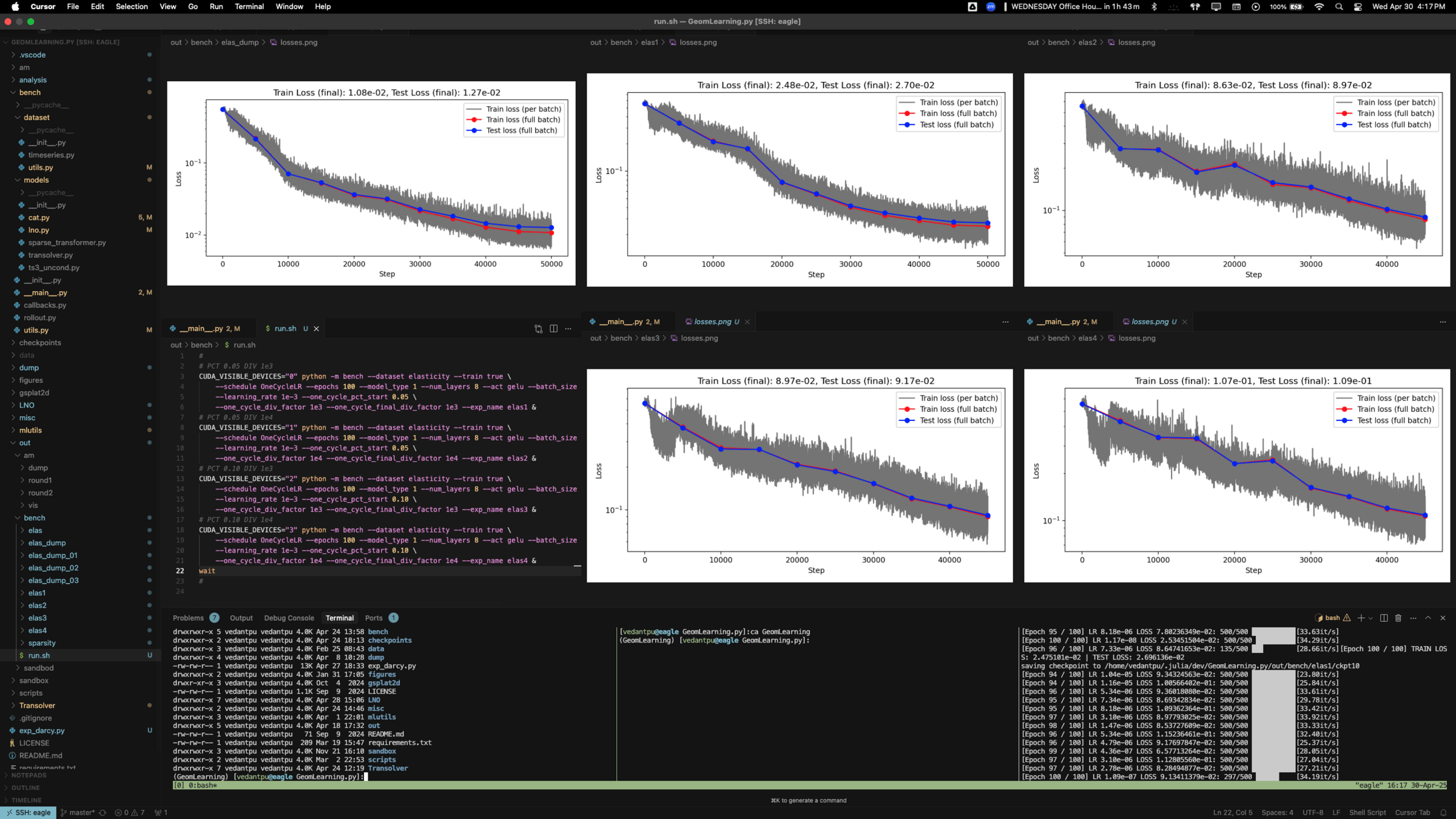
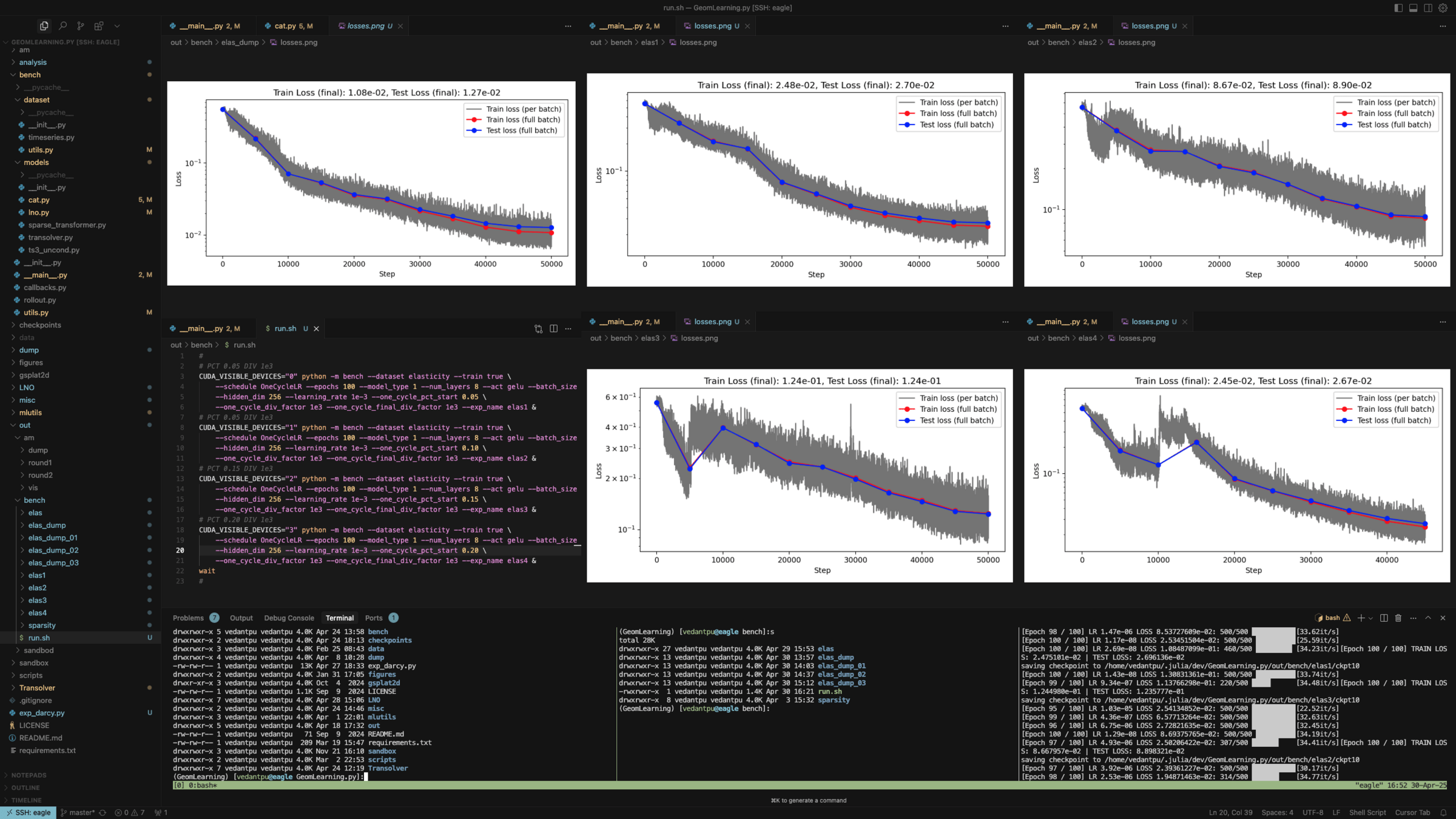
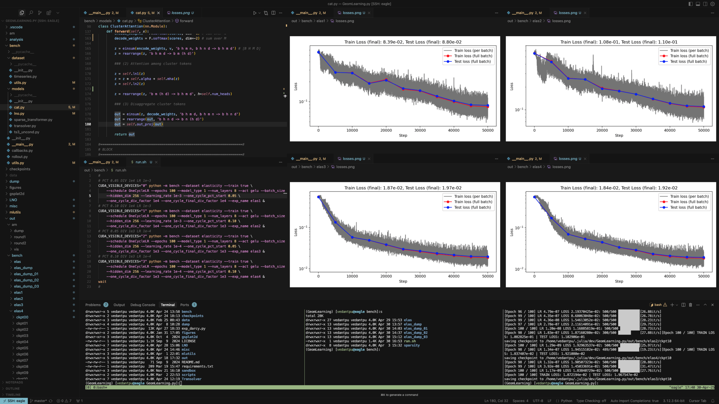
Loss curves
1000 train / 100 test
200 train / 50 test
140 train / 35 test
Transolver (physics attention)
Cluster Attention
| Dataset | CA + Concat | CA + AdaLN | CA + Q-Cond | TS + Concat | TS + AdaLN | UPT | GINO |
|---|---|---|---|---|---|---|---|
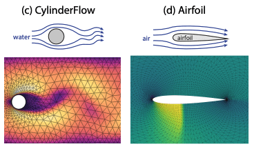
| Cylinder Flow | |||||||
| Airfoil | |||||||
| ... | |||||||
| AM Dynamic |
| Dataset | Cluster Attention (CA) | Transolver (TS) | UPT | GINO |
|---|---|---|---|---|
| Elasticity | ||||
| Darcy | ||||
| ... | ||||
| AM steady |
Dynamic rollout comparison
Steady state comparisons
Maybe we should forego Adaptive layer-norm for the same of time
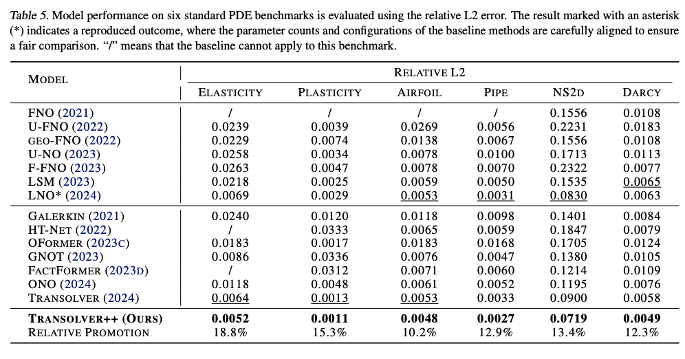
| LNO (from their paper) | 0.0052 | 0.0029 | 0.0049 | 0.0026 | 0.0845 | 0.0049 |
|---|
| Cluster Attention (ours) | 0.0040 | - | - | - | - | - |
|---|
| Our impl of transolver | 0.0064 | - | - | - | - | - |
|---|
| unified_pos \ deriv_loss | True | False |
|---|---|---|
| True | 0.005969 | 0.00638390 |
| False | - | 0.00679797 |
Darcy experiments with transolver (conv2D) on transolver repo
| unified_pos \ deriv_loss | True | False |
|---|---|---|
| True | 0.00612938 | 0.0070930 |
| False | 0.0075420 | 0.0076147 |
Darcy experiments with transolver (conv2D) on transolver repo with max_grad_norm=None
| Setup | Train MSE | Test MSE | Train Rel Error | Test Rel Error |
|---|---|---|---|---|
| TS conv BS 4 OCLR 1e-3 E 500 CGN 1e-1 | - | - | - | 0.0057543 |
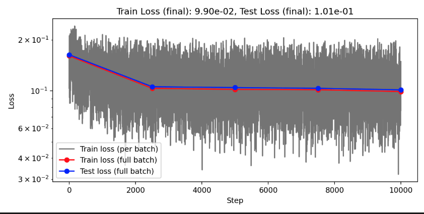
| CA conv BS 4 OCLR 1e-3 E 500 CGN 1e-0 | 9.48e-4 | 2.52e-3 | 0.0048791 | 0.0072914 |
| CA conv BS 4 OCLR 5e-4 E 500 CGN 1e-0 | 7.03e-4 | 2.68e-3 | 0.0042424 | 0.0073877 |
| CA conv BS 2 OCLR 5e-4 E 500 CGN 1e-0 | - | - | - | |
| CA conv BS 2 OCLR 1e-4 E 500 CGN 1e-0 | 4.45e-4 | 2.07e-4 | 0.0032965 | 0.005795 |
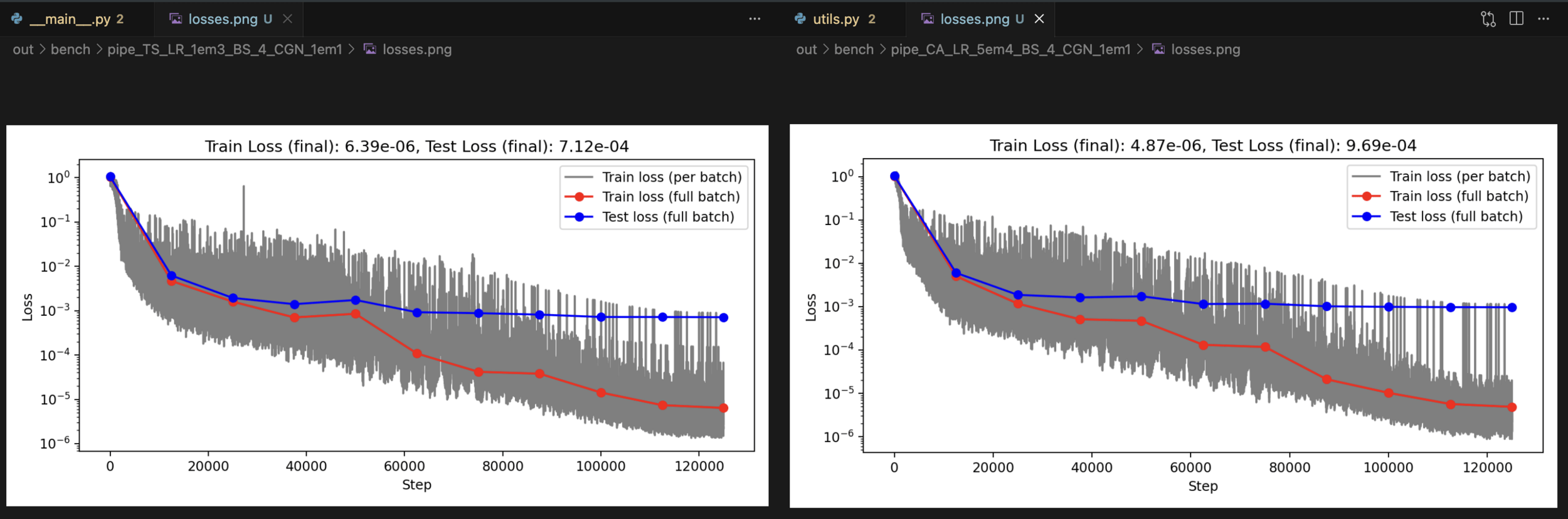
Cluster Attention w/o conv
Transolver w/o conv
| Setup | Train MSE | Test MSE | Train Rel Error | Test Rel Error |
|---|---|---|---|---|
| TS conv BS 2 LR 1e-3 E 500 CGN 1e-1 WD 1e-5 | 0.0045 | |||
| TS conv BS 4 LR 1e-3 E 500 CGN 1e-1 WD 1e-5 | 6.39e-6 | 7.12e-4 | 0.000998 | 0.00462 |
| CA conv BS 4 LR 1e-3 E 500 CGN 1e-0 WD 1e-5 | 3.62e-4 | 1.82e-3 | 0.007495 | 0.011562 |
| CA conv BS 4 LR 5e-4 E 500 CGN 1e-0 WD 1e-5 | 7.38e-6 | 8.94e-4 | 0.0010101 | 0.00565 |
| CA conv BS 4 LR 5e-4 E 500 CGN 1e-1 WD 1e-5 | 4.87e-6 | 9.69e-4 | 0.000840 | 0.00576 |
| CA conv BS 2 LR 5e-4 E 500 CGN 1e-1 WD 1e-5 | ||||
| CA conv BS 2 LR 1e-4 E 500 CGN 1e-1 WD 1e-5 | ||||
| CA conv BS 2 LR 1e-4 E 500 CGN 1e-1 WD 1e-4 |
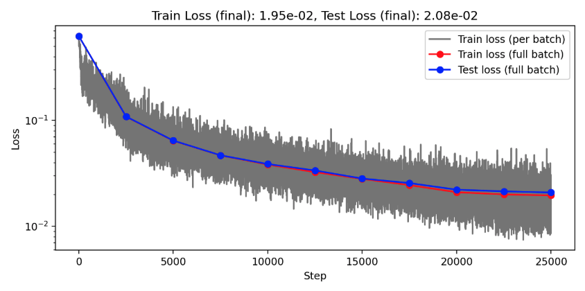
Transolver H = 128, Conv2D = False
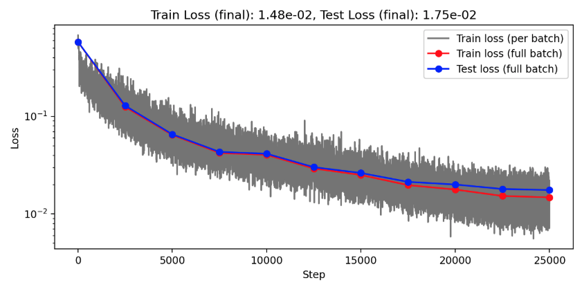
Cluster Attention H = 128, Conv2D = False
Transolver H = 256, Conv2D = False
Cluster Attention H = 256, Conv2D = False
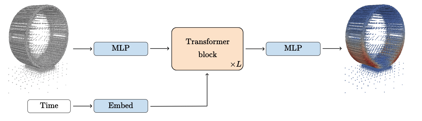
Modeling dynamical deformation in LPBF with neural network surrogates
Spatial Discretization
Temporal Discretization
GNN / Transformer
Transformer embedding
Neural implicits
Naive next step prediction
LSTM
Transformer next step prediction
Nonlinear kernel parameterizations for Neural Galerkin
Status and plan
Potential new contributions and timeline
Parameterized Tanh kernels
Nonlinear kernel parameterizations for Neural Galerkin
Status and plan
Potential new contributions and timeline
Parameterized Tanh kernels
Parameterized Gaussian (OURS)
3 parameters
8 collocation points
Deep Neural Network (BASELINE)
~150 parameters
256 collocation points
Multiplicative filter network (MFN)
~210 parameters
256 collocation points
Error due to limited expressivity of this simple model
FAILED TO CONVERGE
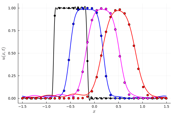
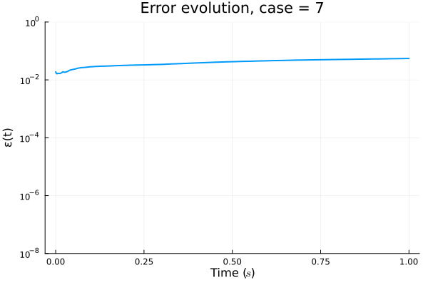
1 Kernel (6 params)
4 Kernel (21 params)
By Vedant Puri
Biweekly co-advisor meeting


