

Vedant Puri
PhD student at Carnegie Mellon University
SEPT 8, 2022
Vedant Puri
Advisor: Venkat Viswanathan
Mechanical Engineering PhD Qualifying Examination
Carnegie Mellon University
LinearSolve.jl
Need analytical forms of all sources and sinks!
Residual physics
Ground truth
Analytical form
Goal: Embed symmetry-representing functions (neural networks) inside conservation laws to learn residual physics.
Conservation Laws
Symmetries (Noether's theorem)
| Conservation Law | Symmetry |
|---|---|
| Linear momentum | Translation |
| Angular momentum | Rotation |
| Time | Energy |
Navier-Stokes system
(Pandya, 2013)
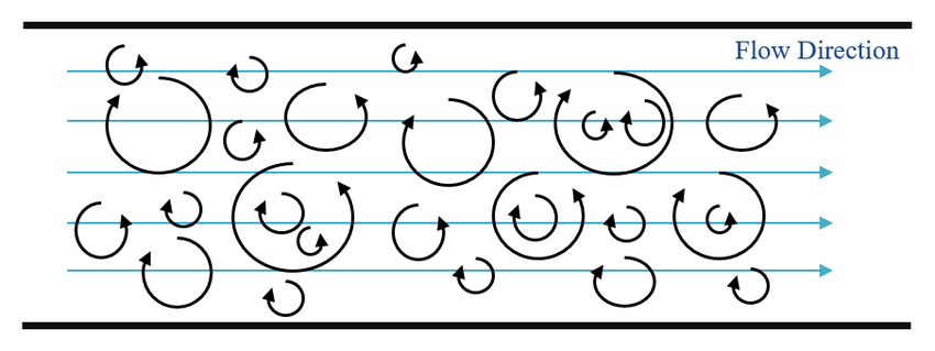
Mode coupling
Closure model
Filtering
Large Eddy Simulation equations
Aim: Develop a framework to embed symmetry-respecting functions inside governing equations to improve closure models.
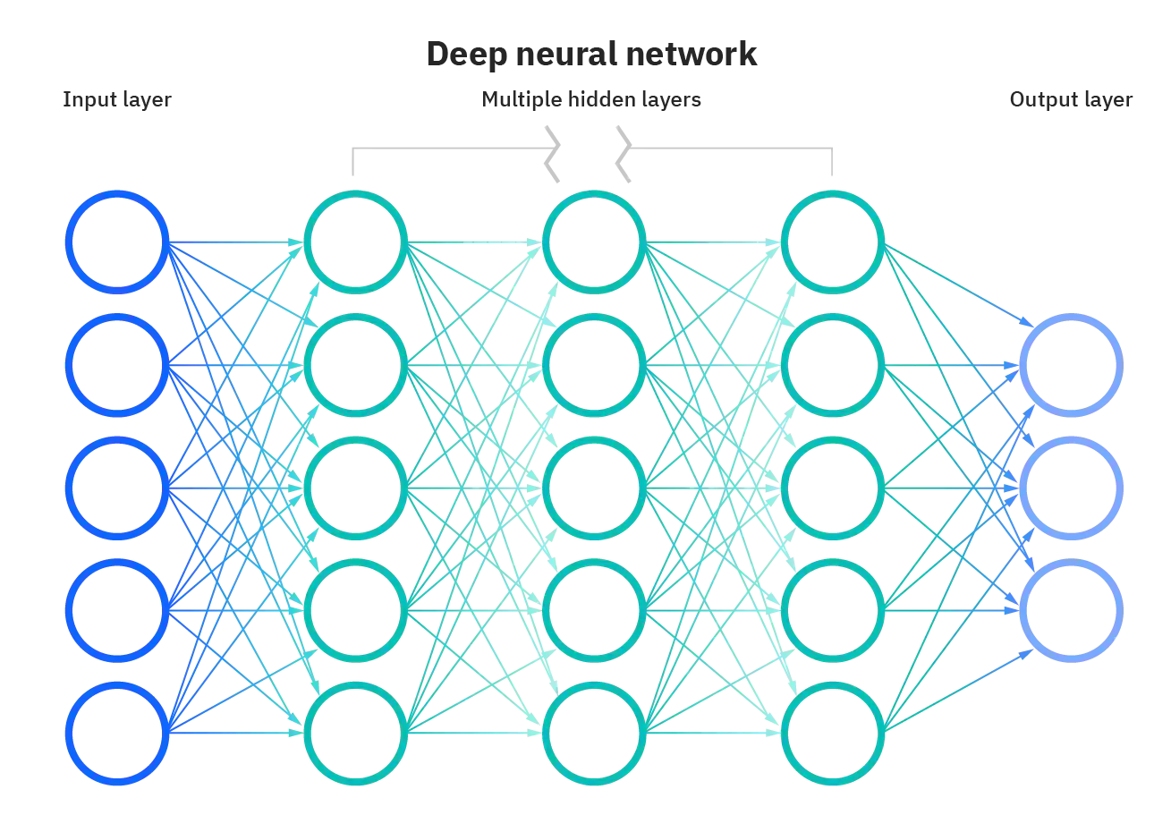
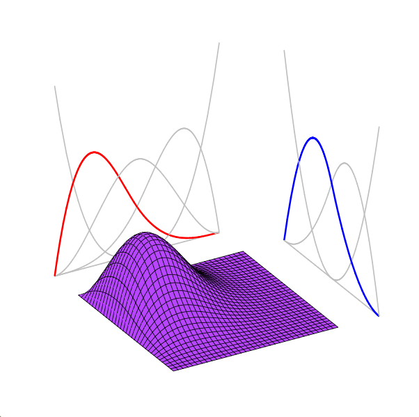
| Orthogonal Functions | Deep Neural Networks |
|---|---|
|
|
|
|
|
|
|
|
\( N \) parameters, \(M\) points
\( h \sim N^{-c/d} \)
\( h \sim 1 / N \) (for 2-layer networks)
\( N \) points
\( \dfrac{d}{dx} \tilde{f}\sim \mathcal{O}(N^2) \) (exact)
\( \dfrac{d}{dx} \tilde{f} \sim \mathcal{O}(N) \) (exact, AD)
\( \int_\Omega \tilde{f} dx \sim \mathcal{O}(N) \) (quadrature, exact)
(Weinan, 2020)
\( \int_\Omega \tilde{f} dx \sim \mathcal{O}(M) \) (Monte-Carlo, approx)
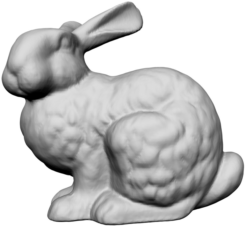
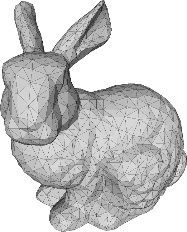
Mesh
Challenge: Embed ML inside PDE problems
\(A\underline{u} = M\underline{b} \)
Domain
Governing Equation
Boundary Constraint
\( NN_\theta \)
Discretization
\( \dfrac{d}{dt} \underline{u} = f(\underline{u}) \)
Solving
Discrete Problem
\(u(\underline{x},t) \)
\(u(\underline{x}) \)
Time-Stepper
Linear Solver
Solution
Loss
Backpropogation
Ground truth
\( NN_\theta \)
\( NN_\theta \)
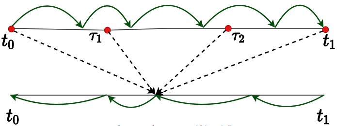
Interpolating Adjoint Method for ODEs
Forward pass
Backward pass
(Daulbaev, 2020)
(Johnson, 2006)
Adjoint Method for linear systems
AD tools are incomplete
Meshing
Linear System
A\(Mf)
Sparse
Structured
+
+
PDE System
Boundary Data
Function Space
Solve Scheme
Iterative Solver
Enforce Locality
Cheap
Domain
Strategy: Build out a unified PDEs ecosystem for Julia SciML!
Abstractions
Composable
AD support
Fast solvers
DL ecosystem
Large (NNs + solvers)
Multiple discretizations
Wants
Fast adjoints
Method
Interoperability
Optimized methods
High performance
High level
General unified interface
Wrap SOTA solvers
ML based discrs
using LinearSolve, LinearAlgebra
A = rand(1000, 1000)
b = rand(1000)
prob = LinearProblem(A, b; u0=zero(1000))
sol = solve(prob)
sol = solve(prob, LUFactorization())
sol = solve(prob, IterativeSolversJL_GMRES())
Pl = Diagonal(A)
sol = solve(prob, KrylovJL_CG(), Pl=Pl,
            abstol=1e-8, maxiters=20)

cache = init(prob)
sol = solve(cache)

cache = LinearSolve.set_b(rand(1000))
sol2 = solve(cache)

using OrdinaryDiffEq, LinearSolve
prob = ODEProblem(A, rand(1000), (0, 1))
sol = solve(prob, SBDF2(
                        linsolve=KrylovJL_GMRES(),
                        precs=incompletelu,
                        tol=1e-8,
                        maxiters=20,
                       )
Unified, general, interface over linear solvers in Julia
\(\texttt{LinearSolve.jl}\) sped up large stiff PDEs solves in \(\texttt{SciML}\) ecosystem!
Adjoint support over interface
Cache reuse
Wraps it all!
Expose solver choice to user in downstream packages
using AbstractPDEInterfaces, NodalPolynomialSpaces

N = 64
ν = 0.01

xdom = IntervalDomain(-1, 1, boundary_tags=(:left, :right))
ydom = IntervalDomain(-1, 1, boundary_tags=(:lower, :upper))
dom = xdom ⊗ ydom

space = GaussLobattoLegendreSpace(N, N; dom=dom)
(x, y,) = points(space)

bcs = Dict(
           :left => NeumannBC(),
           :right => DirichletBC(),

           :lower => DirichletBC(),
           :upper => NeumannBC(),
          )

discr = Galerkin()
lhsOp = diffusionOp(ν, space, discr)

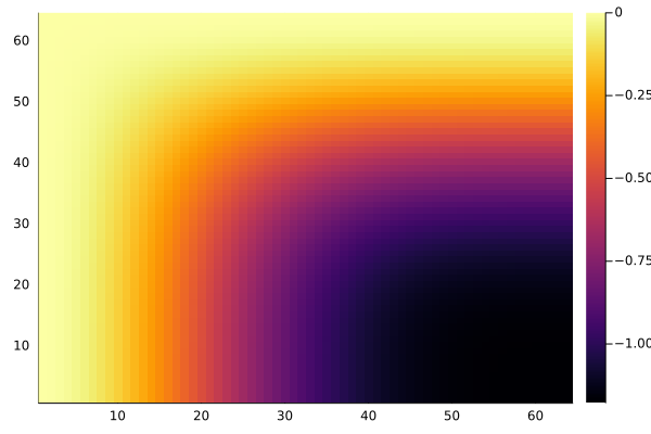
f = @. 0*x + 1

prob = BoundaryValueProblem(lhsOp, f, bcs, space, discr,
                            abstol=1e-8, reltol=1e-8)

alg  = LinearBoundaryValueAlg(linalg=KrylovJL_CG())

@time sol = solve(prob, alg; verbose=false)
# 0.201703 seconds (39.71 k allocations: 49.417 MiB)
@test sol.resid < 1e-8
# Test Passed
Plug & play
modular
Domains
Function Spaces
\( \texttt{FourierSpaces.jl} \)
Solve schemes
Boundary constraint
Galerkin
Collocation
Rectangular
Mapped
Dirichlet
Neumann
\( \texttt{CalculustCore.jl} \)
*wip
Meshed*
Implicit*
\( \texttt{SpectralElementSpaces.jl} \)*
Periodic*
Robin
\( A \underline{u} = M \underline{b} \)
\( \dfrac{d}{dt}\underline{u} = f(\underline{u}) \)
\( \texttt{NodalPolynomialSpaces.jl} \)
\( \texttt{SciMLOperators.jl} \)
\( \texttt{LinearSolve.jl} \)
\( \texttt{OrdinaryDiffEq.jl} \)
CalculustJLClosure Model
Deterministic
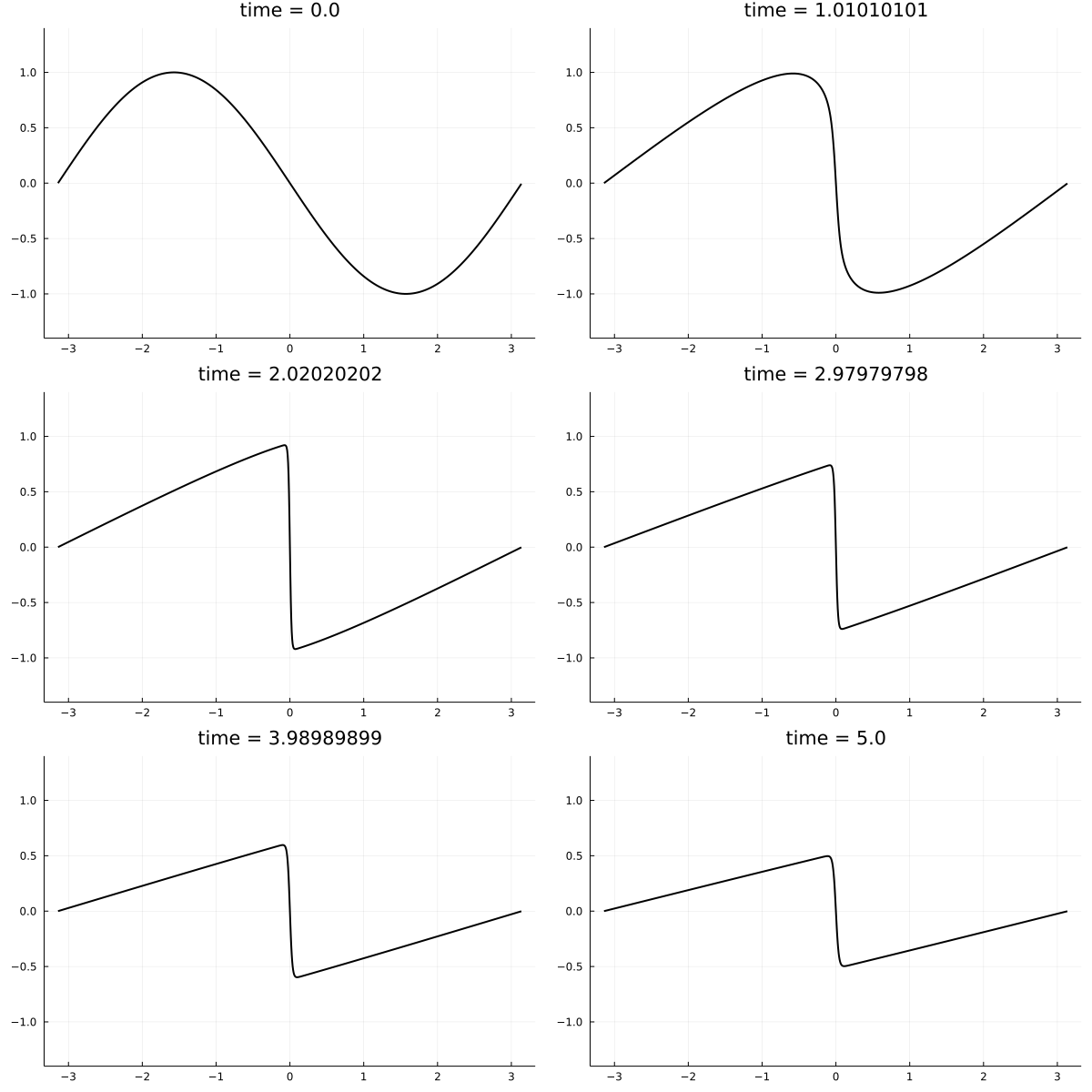
Shocks
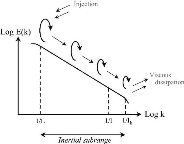
Energy Cascade
Eddy Viscosity Model
Vanilla Neural Network
Eddy Viscosity Model
Transport Equation Model
Eddy Viscosity with Transport
Vanilla Neural Network
SciMLOperators.jlI see \(\texttt{CalculustJL}\) as the overarching outcome of my PhD. Plan to have future work compatible with and extend the interface
Governing System
Boundary Data
Time Domain
** stationary
* continuum scale
Space Domain
- Setting up is hard because you have to read geometry from CAD/ scans.
- Mesh has to accurately represent geom
- Obtaining physically correct initial and boundary conditions from data
- Solving is hard because we end up with large linear systems
- Critically, quality of mesh dictates time to solution. Mesh iteration is time consuming. Geom respecting meshes are v large
- Asserting BC is nontrivial
- Massive systems of equations. Large compute requirements
Autodiff: compiler magic that gives bwd pass based on chain rule. Lets you modify parameters past nonlinearities
Tackle deeply nested, high dim problems in computational workflows with DiffPhys
By Vedant Puri
Turbulence closure modeling with differentiable physics