
On Generating Orthogonal Polynomials

DEC 7, 2022

Vedant Puri

https://github.com/vpuri3

Mechanical Engineering, Carnegie Mellon University

Agenda

  • Motivation: PDE Solvers
  • Polynomial Interpolation
  • Orthogonal Polynomials
  • Properties
  • Generating polynomials

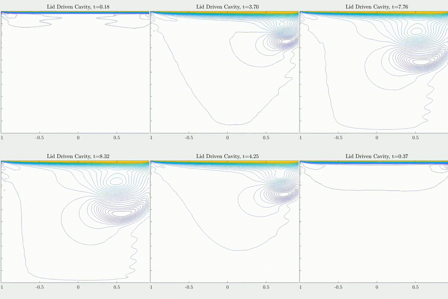
PDEs solvers are needed for predictive modeling

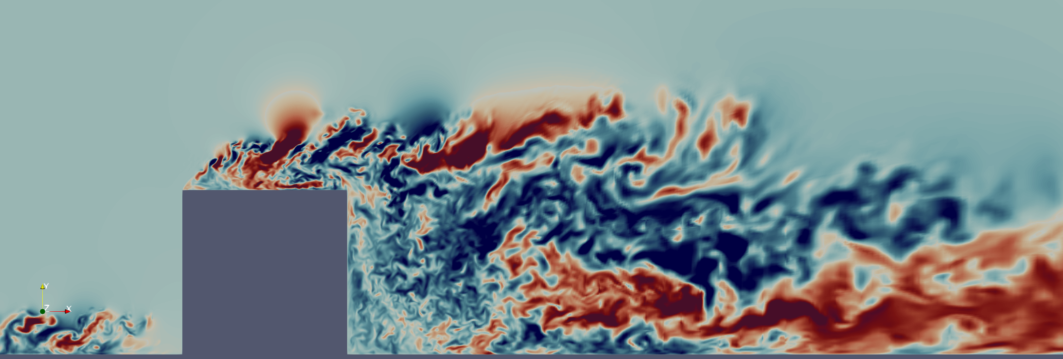
\partial_t \vec{v} + (\vec{v}\cdot\nabla)\vec{v} = -\nabla p + \frac{1}{\text{Re}}\Delta \vec{v} + f\\ \nabla\cdot\vec{v} = 0

Navier-Stokes Equations

(Flow past bluff body \( Re = 3900 \))

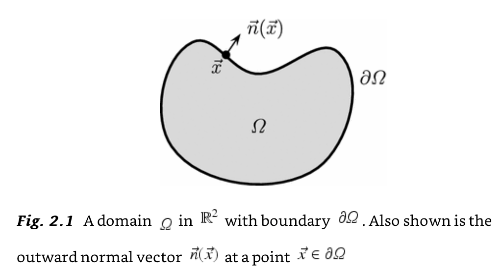
Need high quality function representation over (complex) geometry.

Main operations: \(\nabla, \, \int_\Omega\)

High-order interpolation is the underlying technology

With a basis over \(\Omega\),

\{ \phi_0(x), \, \phi_1(x), \cdots \phi_{N-1}(x) \}
\frac{\mathrm{d}}{\mathrm{d} x} f(x) = \Sigma_{n=0}^{N-1} f_i \frac{\mathrm{d}}{\mathrm{d} x} p_n(x)
\int_\Omega f(x) \mathrm{d} x = \Sigma_{n=0}^{N-1} f_n \int_\Omega p_n(x) \mathrm{d} x

Functions can be written as expansions

f(x) = \Sigma_{n=0}^{N-1} f_i p_n(x)

\(\nabla, \, \int\) can be done on the basis

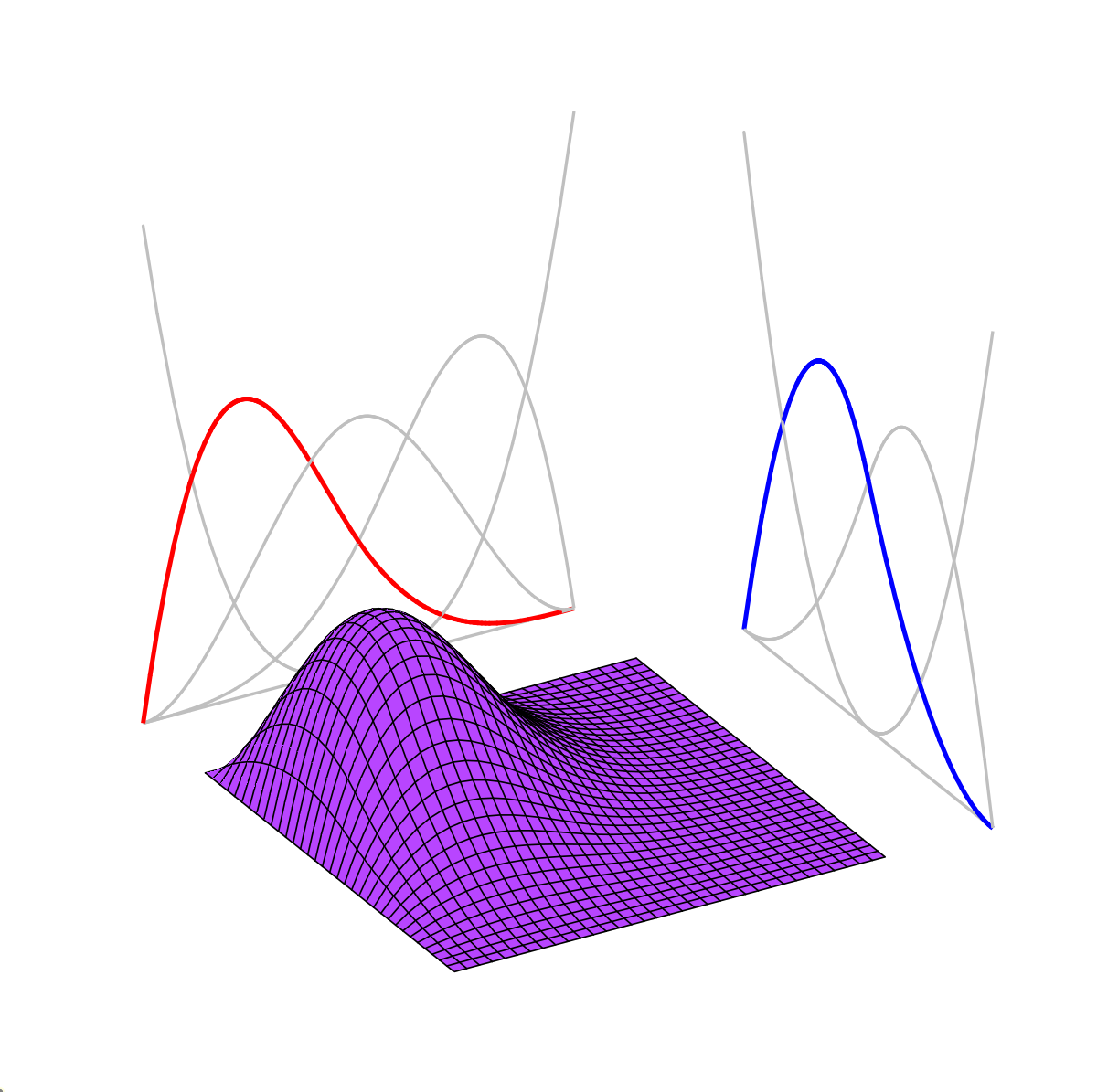
(Tensor-product basis)

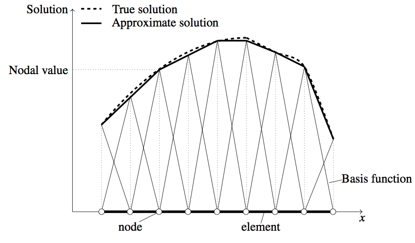
(Linear Finite Element basis functions)

Exact

Fast

Properties of the basis are endowed on to the function

Well-conditioned

Lagrange interpolants and Gauss Quadrature are all we need

For a set of nodes

\{ x_0, \, x_1, \, \cdots, x_{N-1} \}

Lagrange Polynomials can be defined

\ell_i(x) = \frac{\prod_{j\neq i}x - x_j}{\prod_{j\neq i} x_i - x_j}
\ell_i(x_j) = \delta_{ij}

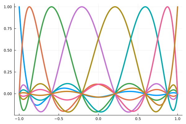
(Lagrange Polynomials over Gauss-Lobatto-Legendre nodes)

Differentiation

Interpolation

What about integration?

For a special set of nodes

\int_\Omega w(x)f(x) \mathrm{d} x = \sum_{n=0}^{N-1} w_n f(x_n)

Integration

Gauss Quadrature

\(\{x_n\}_n\) are roots of the \(n^\text{th}\) orthogonal polynomial generated by \(w(x)\) in \(\Omega\).

Conditioning

Orthogonal Polynomials

\{ 1, x, x^2, x^3, \cdots, x^{N-1} \}
\langle p_i, p_j \rangle = \int_a^b p_i(x) p_j(x) \underbrace{w(x) \mathrm{d}x}_{\mathrm{d}\alpha}

Orthogonalization

(Gram-Schmidt)

Start with the monomials

Orthogonal WRT inner product on \( C(\mathbb{R}) \)

\{ p_0(x), p_1(x), \cdots, p_{N-1}(x) \}

\(w(x)\) generates a unique family of orthogonal polynomials (up to normalization)

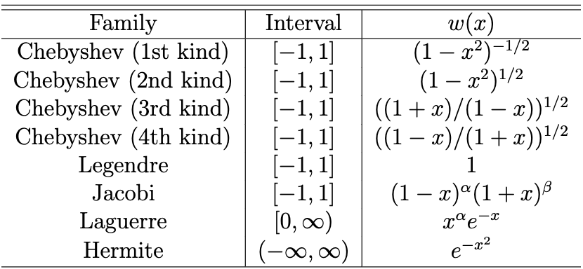
(Classical Orthogonal Polynomials)

Sturm-Louisville Theory

\frac{\mathrm{d}}{\mathrm{d} x}\left( p(x) \frac{\mathrm{d} }{\mathrm{d} x}\phi(x) \right) + q(x) \phi(x) = -\lambda w(x)\phi(x),\\ x\in\Omega, + \,\text{BC}

Classical Orthogonal Polynomials emerge as solutions to the Sturm-Louisville problem

Example: Fourier (trigonometric) polynomials are the eigenfunctions of the Laplace equation

-\frac{\mathrm{d}^2}{\mathrm{d}x^2}\phi(x) = \lambda \phi(x), \, x\in(-1,1)\\ u|_{-1} = u|_{1}
\phi_{n}(x) = \sin(n\pi x) + \cos(n\pi x)\\ \lambda_n = n^2

But boundary condition is embedded in the interpolants. So they are not general purpose.

Trigonometric polynomials have fast transforms: \( \mathcal{O}(N\log(N)) \)

GOAL: Finding orthogonal polynomials is arbitrary geometries

Want to do calculus in arbitrary geometries

Need orthogonal basis over \(\Omega\):

  1. Gauss quadrature nodes and weights
  2. Interpolation, differentiation operators
  3. Matrices should be sparse, well-conditioned
  4. Method to impose boundary condition

Aim

  1. Develop method to generate orthogonal polynomials in 1 dimension
  2. Extend to multiple dimensions

Problems

  1. High-order polynomials (except in special cases) are nasty for numerical computation
  2. No known recurrence relation in 2D/3D

The three-term recurrence relation

(Favad, 1935) All families of orthogonal polynomials follow a 3-term recurrence relation

T_0(x) = 1\\ T_1(x) = x\\ T_{n+1}(x) = 2x T_n(x) - T_{n-1}(x)

Example: Chevyshev polynomials (first kind)

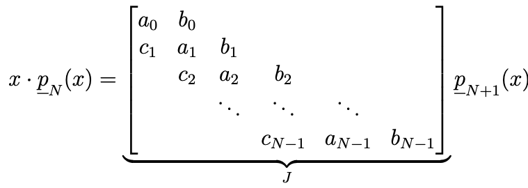
x p_n(x) = c_n p_{n-1}(x) + a_n p_n(x) + b_n p_{n+1}(x)

In general, for \( \{p_n\}_{n=0}^{N-1} \)

In matrix form, we have a tridiagonal system

(Golub & Welsch, 1968) eigenvalues of \(J\) correspond to zeros of \(p_n(x)\).

(Mysovskih, Gautschi) \(J\) is uniquely determined by \(w(x)\)

(Mysovskih, Gautschi) \(J\) is uniquely determined by \(w(x)\)

The moments of the \( w(x) \)

\mu_k = \int_\Omega w(x) x^k \mathrm{d}x

(Golub & Welsch) eigenvalues of \(J\) correspond to zeros of \(p_n(x)\)

Graphs Corresponding to Orthogonal Polynomials

\(p_n(x)\) is the Characteristic poly

Graphs Corresponding to Orthogonal Polynomials

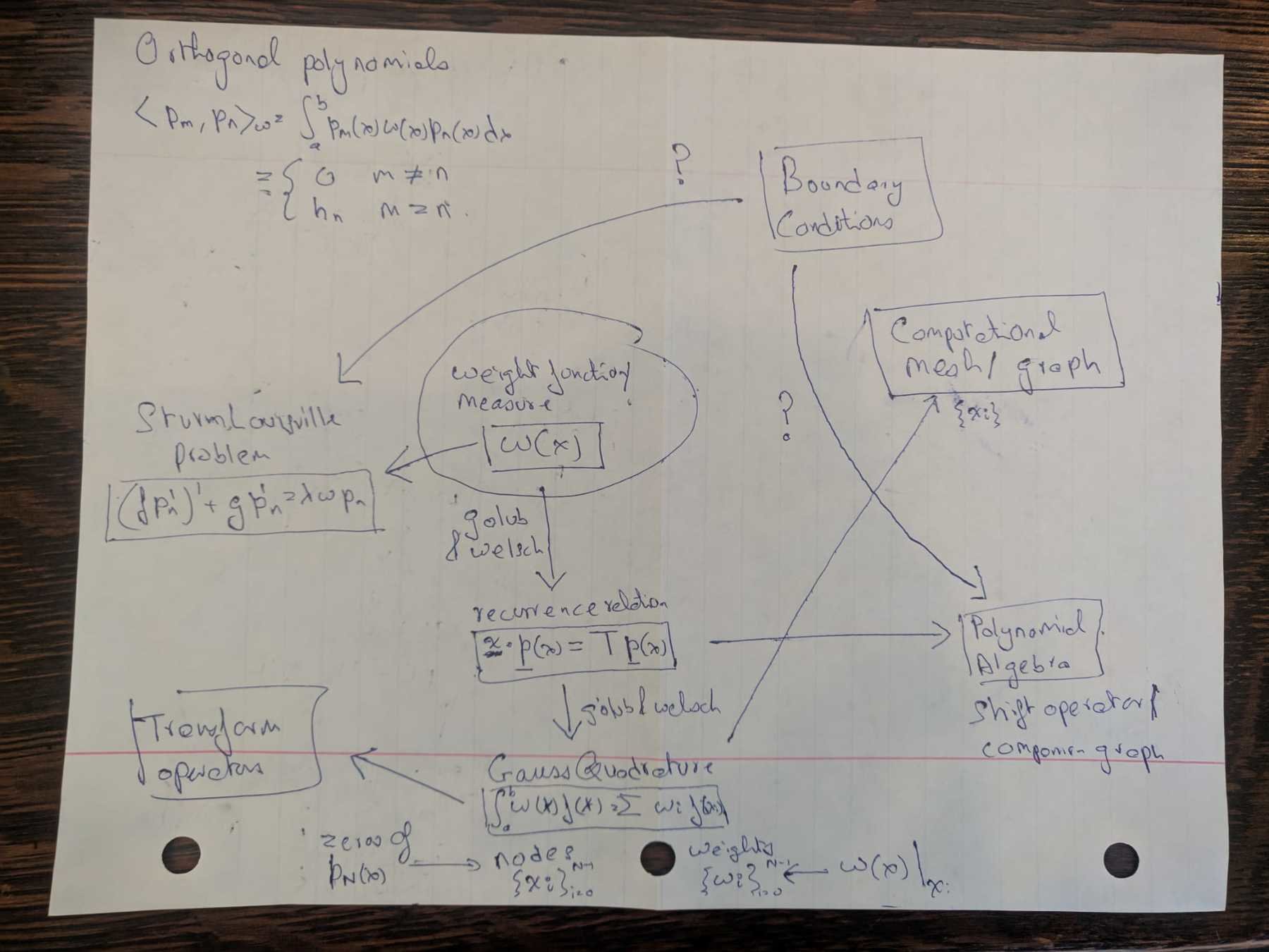
Method

w(x)

Recurrence relation

Gauss Quadrature

Calculus

Conclusions

Implementation Problems

  1. Implementation
    1. High-order polynomials are notoriously ill-conditioned
    2. Gram-Schmidt failing for N > 20
    3. There are methods to get past numerical instability
  2. No guarantee on conditioning of interpolation, differentiation matrix
  3. Mysovskih, Gautschi - algorithm requires moments computation


    Chicken and egg problem - to get Gauss quadrature for integration, you have to do integration

\mu_k = \int_\Omega w(x) x^k \mathrm{d}x

Thanks

orthogonal_polynomials

By Vedant Puri

orthogonal_polynomials

Orthogonal Polynomials

  • 33