Fluid Dynamics and Turbulence Modeling

SEPT 8, 2022

Vedant Puri


Mechanical Engineering, Carnegie Mellon University

Agenda

  • Fluid Dynamics
    • Navier-Stokes
    • Turbulence
  • Turbulence Modeling
    • Subgrid Stress

Introduction

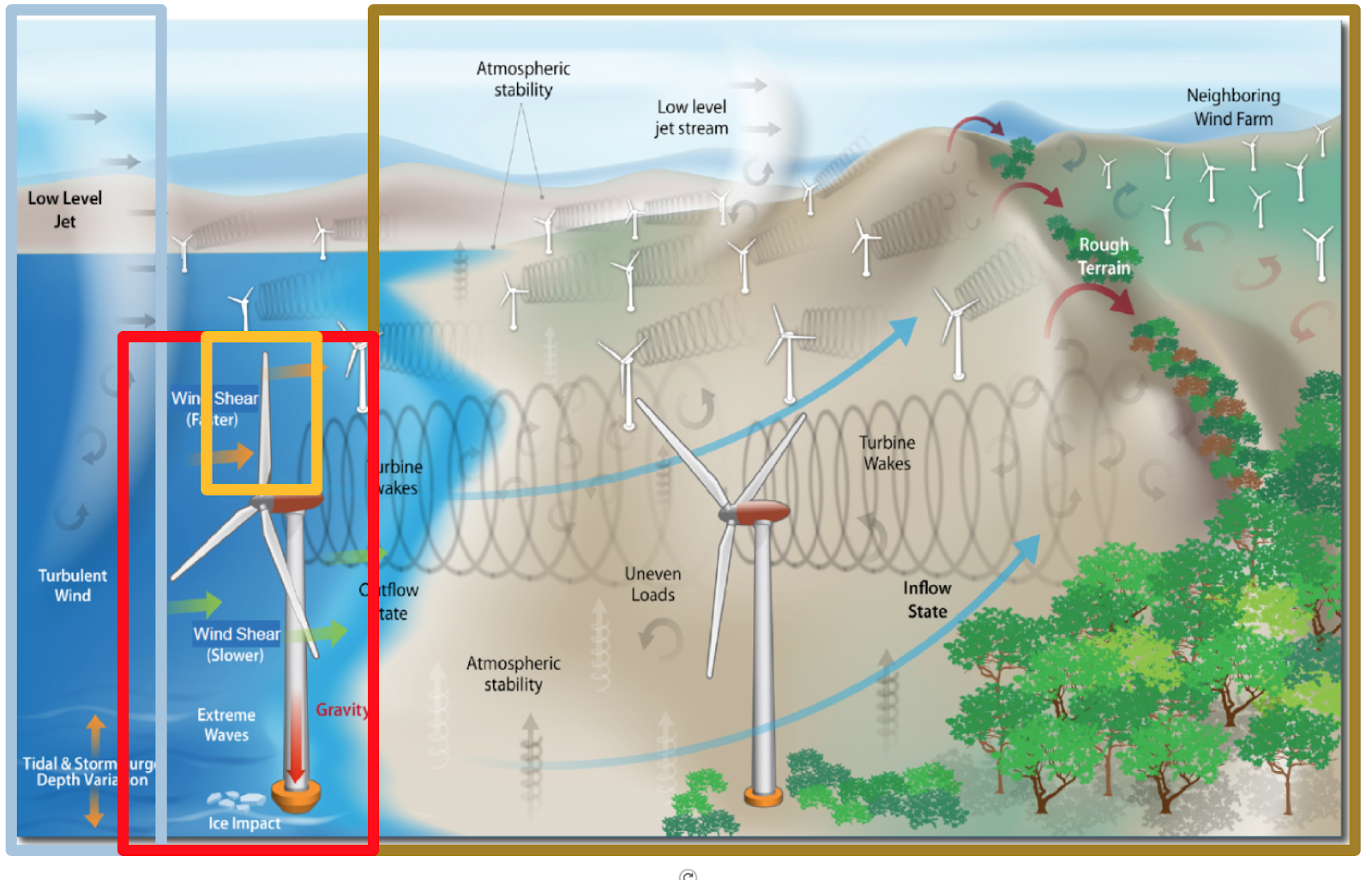
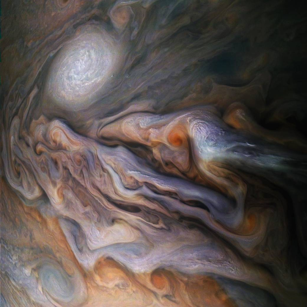
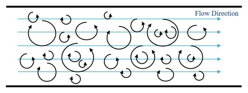
Turbulence is a multiscale phenomena

Mesosphere

Wind farm

Turbine

Blade

(eere.energy.gov)

1000\,\mathrm{km}
10\,\mathrm{km}
100\,\mathrm{m}
10\,\mathrm{m}

Fluid flow is governed by the Navier-Stokes model

\partial_t \vec{v} + (\vec{v}\cdot\nabla)\vec{v} = -\nabla p + \frac{1}{\text{Re}}\Delta \vec{v} + f\\ \nabla\cdot\vec{v} = 0
\rho(\partial_t\vec{v} + \vec{v}\cdot\nabla\vec{v}) = -\rho\nabla p + \mu\Delta \vec{v} + \rho f
\nabla\cdot\vec{v} = 0

Reynolds transport theorem

\rho \vec{f}

Lagrangian fluid particle

\rho \vec{v}
\overline{\overline{\tau}}\cdot\hat{n}
p

Incompressible flow

\( \nabla\rho = \vec{0},\, \partial_t\rho=0 \)

\Omega(t)

Newtonian flow

\( \overline{\overline{\tau}} = \frac{\mu}{2}(\nabla\vec{v} + \nabla\vec{v}^T) \)

Momentum conservation (\(F=ma\))

Mass conservation

\text{Re} = \frac{\text{inertial forces}}{\text{viscous forces}} = \frac{U L}{\nu}

Nondimensionalize

Lagrangian \(\iff\) Eulerian

Navier-Stokes is a hard system to solve

\partial_t \vec{v} + (\vec{v}\cdot\nabla)\vec{v} = -\nabla p + \frac{1}{\mathit{Re}}\Delta \vec{v} + f\\ \nabla\cdot\vec{v} = 0,\\ x\in\Omega,\, \mathrm{IC/BC}\\

Simulation

Energy Cascade

Chaotic system

No theory!

Statistical treatment

Singularly perturbed

Thin boundary layers

Geometric nonlinearity

(nasa.gov)

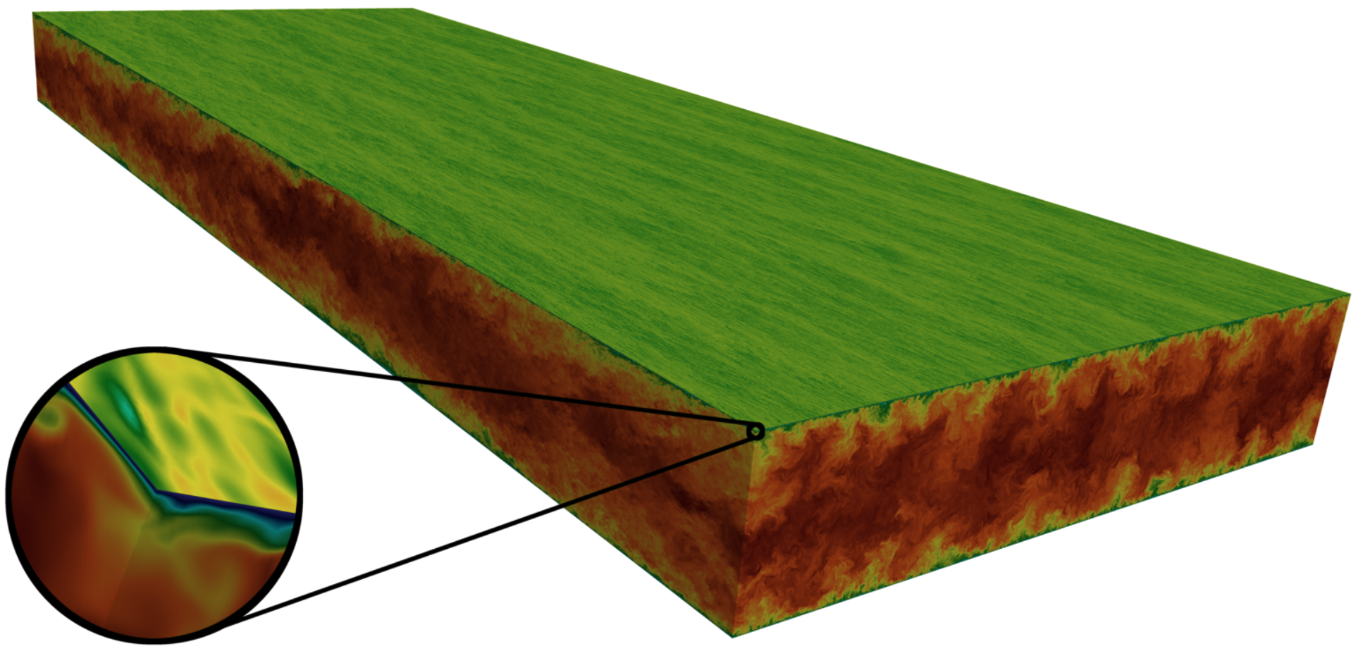
Channel flow at \( \text{Re}=12,500\) (Lee, 2015)

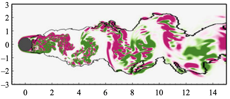
Flow past cylinder at \( \text{Re}=3900\) (Li, 2020)

???

Long time evolution

( wikipedia.org)

Navier-Stokes and Reynolds transport theorem

\rho \vec{f}

Lagrangian fluid particle

\rho \vec{v}
\overline{\overline{\tau}}
p
\Omega(t)
\frac{\mathrm{d}}{\mathrm{d}t}\int_{\Omega(t)} \phi(\vec{x},t)\mathrm{d}\vec{x} = \int_{\Omega(t)}\partial_t \phi + (\vec{v}\cdot\nabla)\phi + \phi(\nabla\cdot\vec{v}) \text{d}\vec{x}

Reynolds transport theorem

Divergence theorem for moving domains

Multidimensional integration by parts

apply to Newton's second law

apply to conservation of mass

Chaos...

How to train chaotic systems? When you can't do trajectory fitting?

Chaos - sensitivity to initial conditions. no two trajectories are the same. must consider statistical averages

Incompressible - stiff pressure poisson solves

infinite speed pressure waves =>

all to all parallel communication =>

discretized system not block-diagonal

Thin boundary layers in advection-dominated limit

Steady advection equation

\partial_t u + v \cdot u_x = \nu u_{xx} + f, x\in[0,L]\\ u|_0 = u|_L = 0
\text{Pe} = \frac{\text{advection transport rate}}{\text{diffusive transport rate}}

boundary layer thickness ~ 1 / Re or something in advection model

\partial_t u + 1 \cdot u_x = \frac{1}{\text{Pe}} u_{xx} + 1, x\in[0,1]

show effect of increasing v at fixed f, Pe.

then show effect of decreasing Pe, fixed v

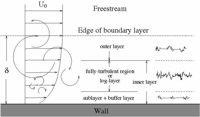
Turbulent boundary layer dynamics

Channel flow at Re=12,500 (Lee, 2015)

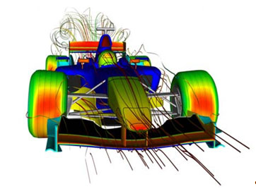
(cfd-online.com)

(su2code.github.io)

Nondimensionalize Navier-Stokes

\mathit{Re} = \frac{\text{inertial forces}}{\text{viscous forces}} = \frac{ma}{\tau_\mu A} = \frac{\rho V\cdot\frac{\mathrm{d} u}{\mathrm{d} t}}{\mu\frac{\mathrm{d} u}{\mathrm{d} y}\cdot A} \propto \frac{\rho L^3\cdot\frac{\mathrm{d} u}{\mathrm{d} t}}{\mu\frac{\mathrm{d} u}{\mathrm{d} y}\cdot L^2} = \frac{\rho L \frac{\mathrm{d} y}{\mathrm{d} t}}{\mu} \propto \frac{\rho U L}{\mu} = \frac{U L}{\nu}
\partial_t \vec{v} + (\vec{v}\cdot\nabla)\vec{v} = -\nabla p + \frac{1}{\text{Re}}\Delta \vec{v} + f\\ \nabla\cdot\vec{v} = 0
\rho(\partial_t\vec{v} + \vec{v}\cdot\nabla\vec{v}) = -\rho\nabla p + \mu\Delta \vec{v} + \rho f
\nabla\cdot\vec{v} = 0

(Nonlinear) advection leads to mode coupling

Inviscid Burgers problem

\partial_t u + u u_x = 0, \, x\in\mathbb{R}

Fourier decomposition

u(x,t) = \sum_{k \in\Z} \hat{u}_{k}(t) \mathrm{e}^{ikx}
\partial_t \hat{u}_k = - \sum_{k = r + s} (is) \hat{u}_r \hat{u}_s

Velocity spectrum interacts with itself!

\partial_t\vec{v} + (\vec{v} \cdot \nabla)\vec{v} = -\nabla p + \frac{1}{\mathit{Re}}\Delta\vec{v} + f

Momentum Equation

To evolve LARGE, you must evolve SMALL!

*energy containing

To resolve any lengthscale, you must resolve every* lengthscale

CFD problems are computationally intractable

Engineering problems are computationally intractable!

( wikipedia.org)

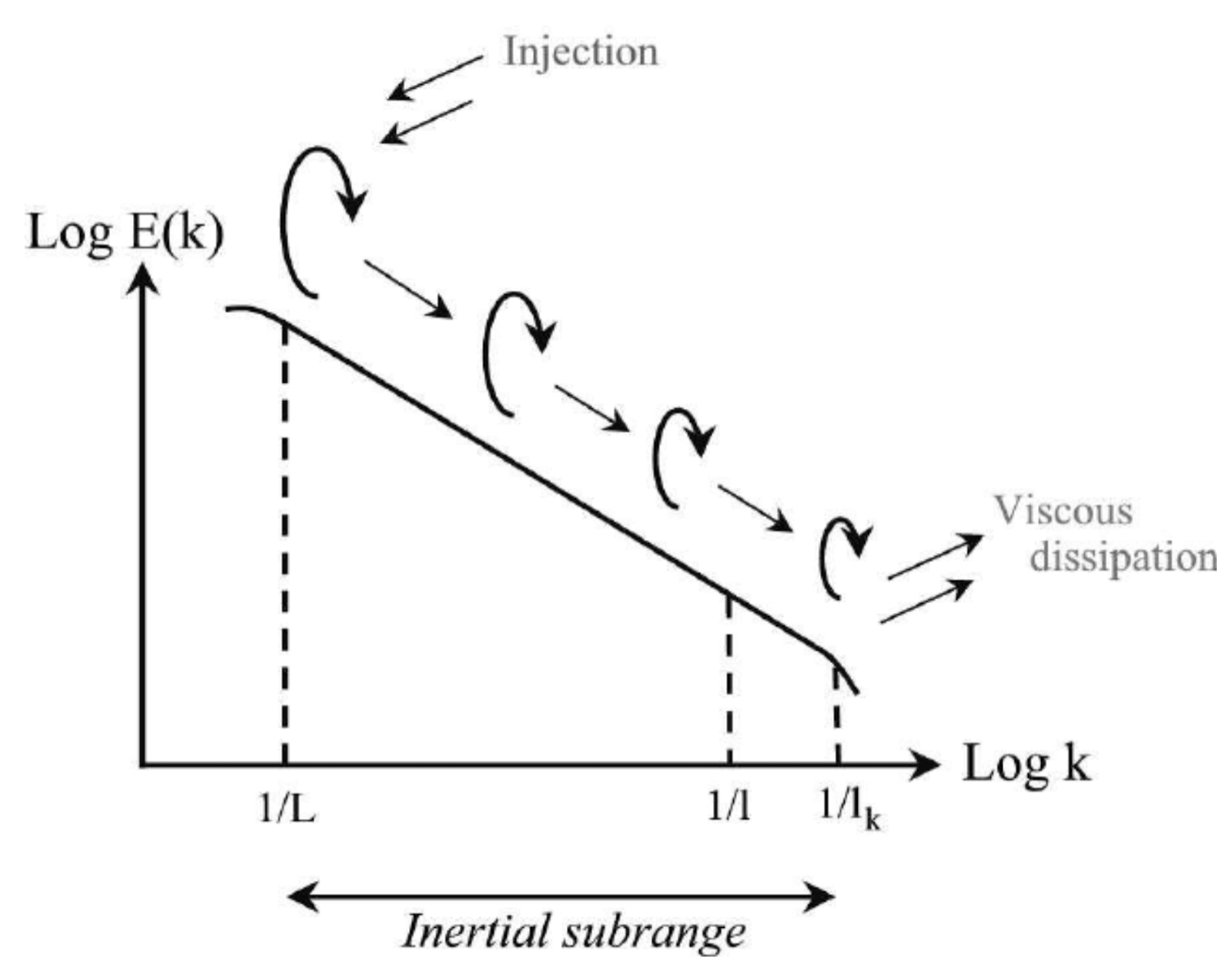
Energy cascade

\lambda
L
\frac{\lambda}{L} \sim \text{Re}^{-3/4}

(Kolmogorov, 1949)

(Pandya, 2013)

N_y \sim \text{Re}^{3/4}
N = N_x \cdot N_y \cdot N_z \sim \text{Re}^{9/4}

Curse of dimensionality!

Superlinear!

Nyquist

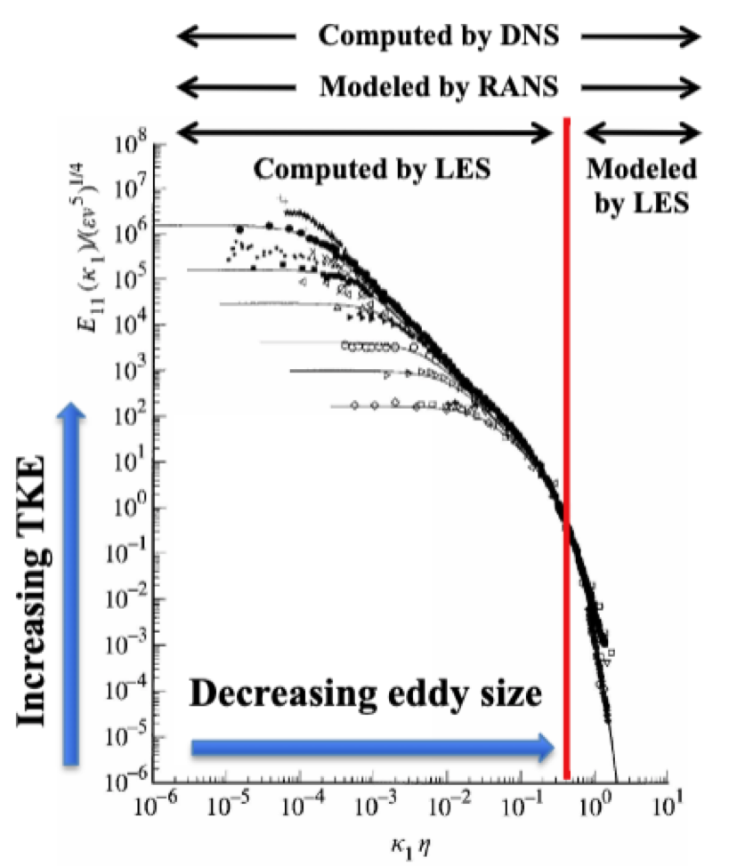
Modeling unresolved scales of turbulent motion

*assuming Moore's law holds

(Spalart, 2012)

\partial_t \bar{v}_i + \bar{v}_j \bar{v}_{i,j} = -\bar{p}_{,i} + \frac{1}{\mathit{Re}}\bar{v}_{i,jj} - \partial_j \overline{v'_i v'_j} \\ \bar{v}_{j,j} = 0
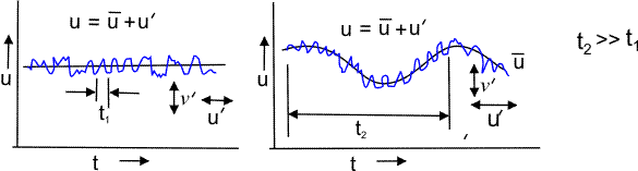
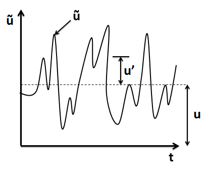
u = \bar{u} + u'

Model!

Modeling subgrid scales of turbulent motion

*assuming Moore's law holds

\partial_t \bar{v}_i + \bar{v}_j \bar{v}_{i,j} = -\bar{p}_{,i} + \frac{1}{\mathit{Re}}\bar{v}_{i,jj} - \partial_j \overline{v'_i v'_j} \\ \bar{v}_{j,j} = 0
u = \bar{u} + u'

Model!

Spalart, Reflections on RANS* Modeling, 2012

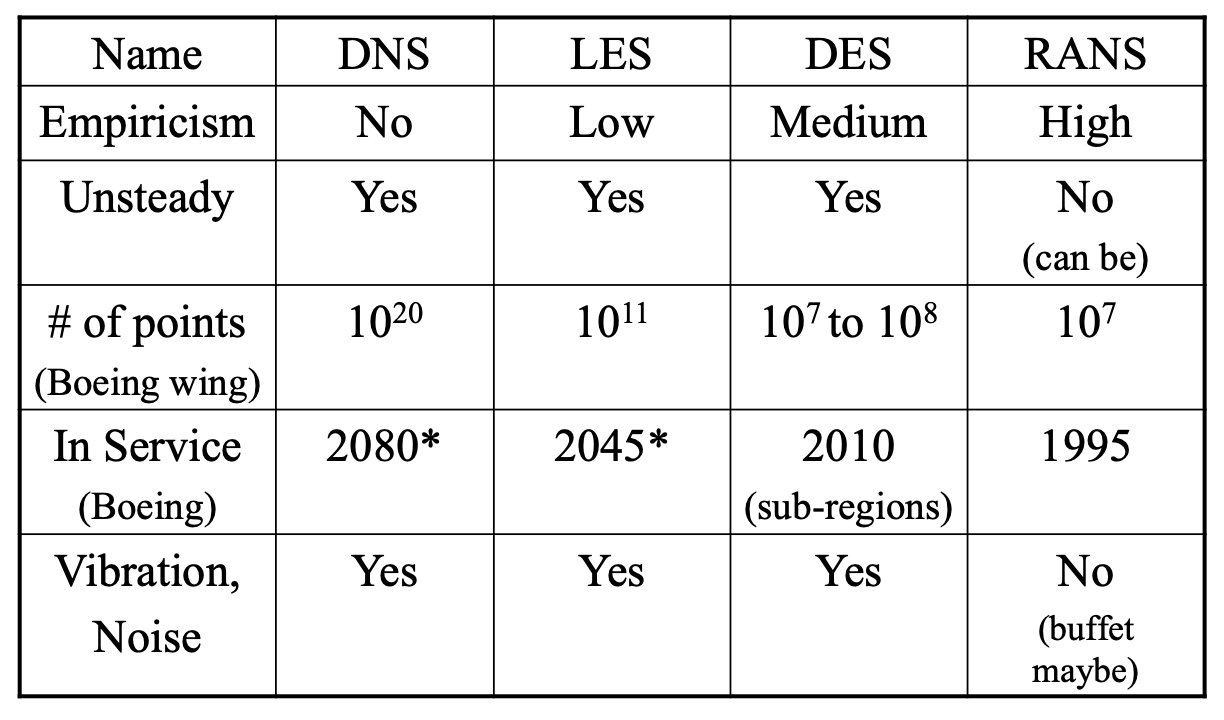
Spectrum of approaches to subgrid modeling

Turbulence Closure Modeling

Navier-Stokes system

\partial_t \vec{v} + (\vec{v}\cdot\nabla)\vec{v} = -\nabla p + \frac{1}{\mathit{Re}}\Delta \vec{v} + f\\ \nabla\cdot\vec{v} = 0

(Pandya, 2013)

Mode coupling

u = \bar{u} + u'
\partial_t \bar{v}_i + \bar{v}_j \bar{v}_{i,j} = -\bar{p}_{,i} + \frac{1}{\mathit{Re}}\bar{v}_{i,jj} - \partial_j \overline{v'_i v'_j} \\ \bar{v}_{j,j} = 0

Closure model

Filtering

Large Eddy Simulation equations

Aim: Develop a framework to embed symmetry-respecting functions inside governing equations to improve closure models.

Fluid Dynamics

By Vedant Puri

Fluid Dynamics

Navier-Stokes and turbulence modeling
  • 33