


Vedant Puri
PhD student at Carnegie Mellon University
1
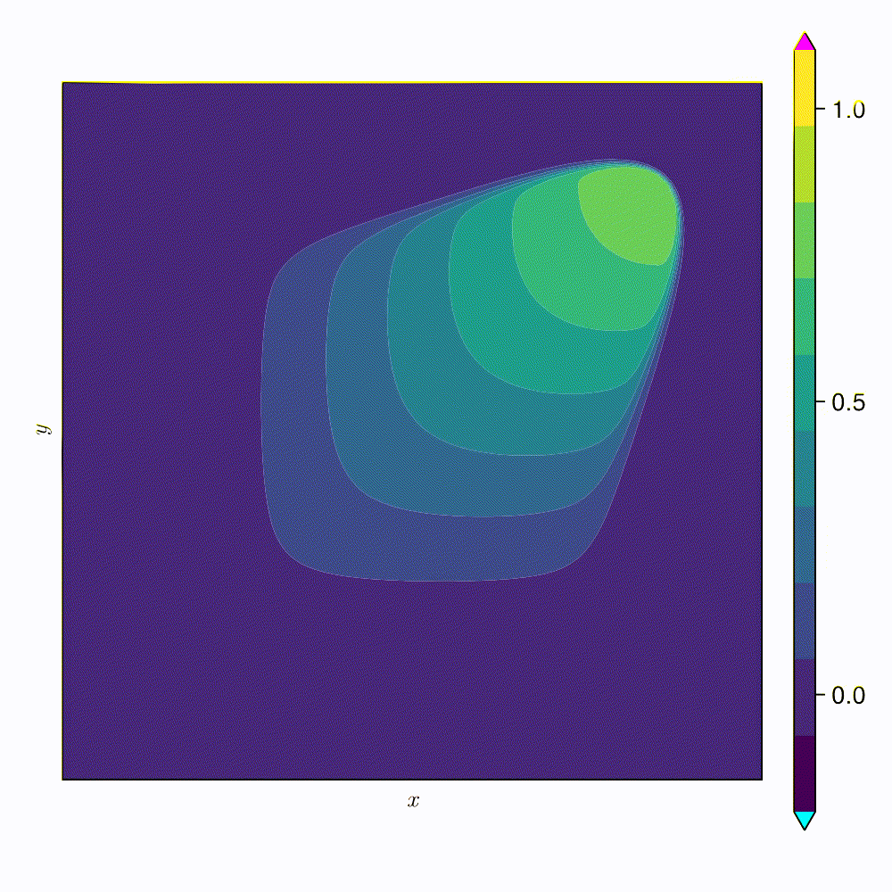
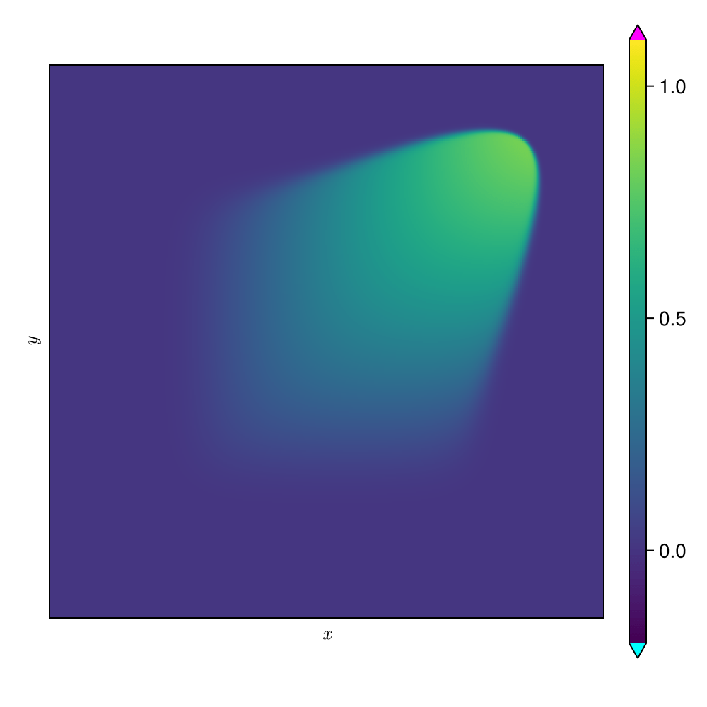
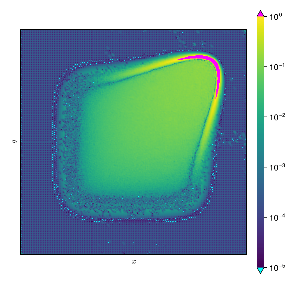
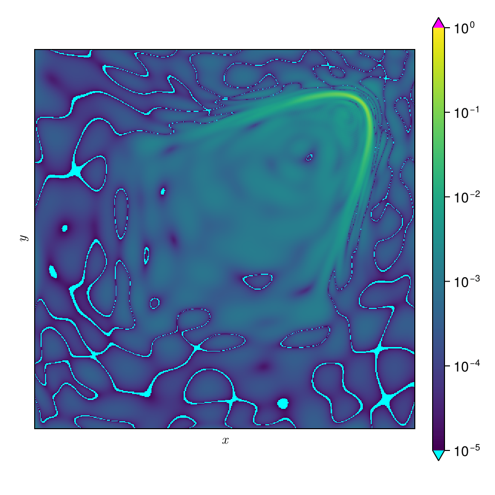
2D Viscous Burgers problem \( (\mathit{Re} = 1\text{k})\)
Smooth neural field ROM (SNF-ROM)
\(\text{Relative error: }0.37\%\)
\(\text{DoFs: }524~k \to 2\)
\(\text{Wall-time: }13.4~\text{s} \to 0.068~\text{s}\)
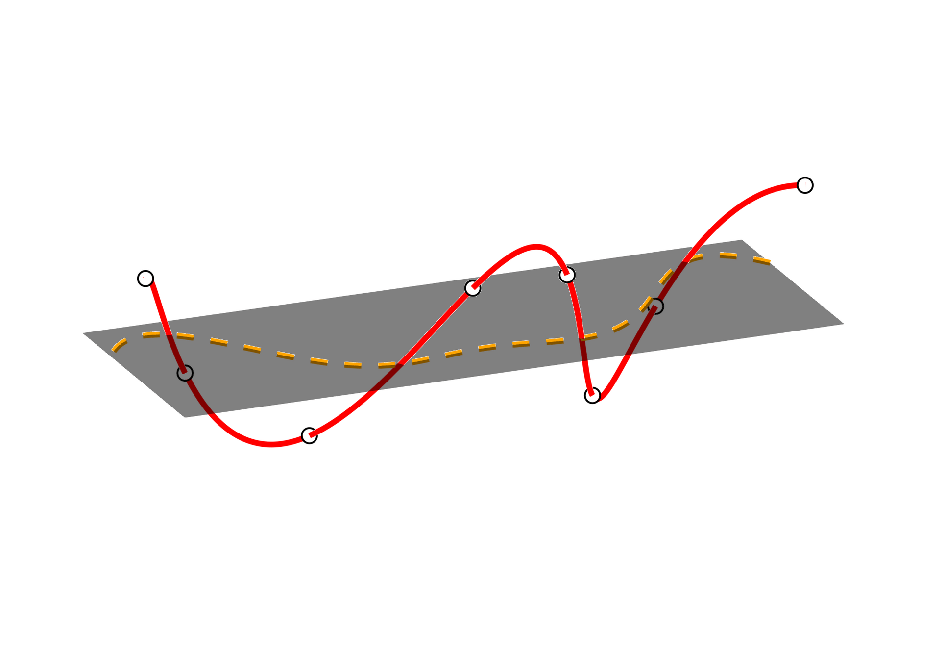
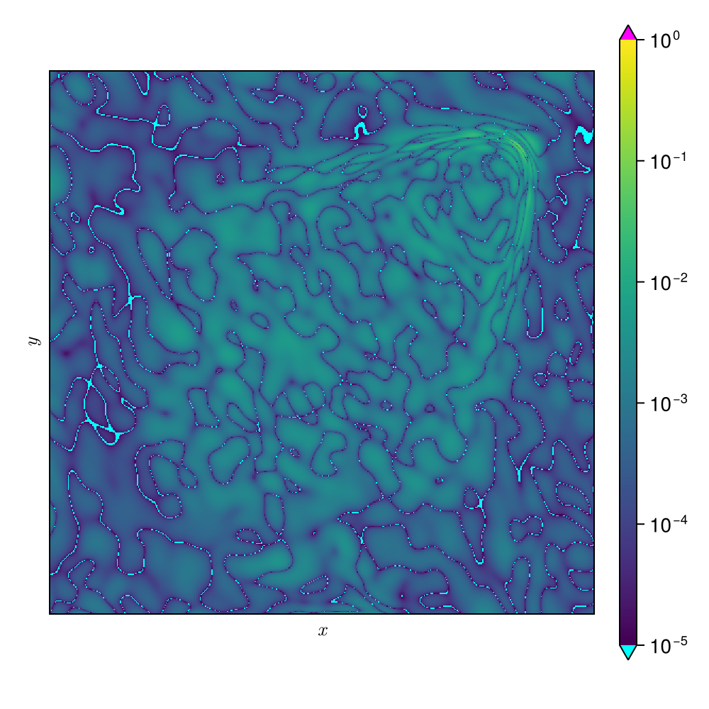
High freq. noise
Non-differentiable!
Accurately capture of dynamics with smooth neural fields
Large deviations!
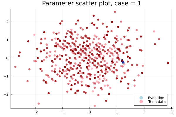
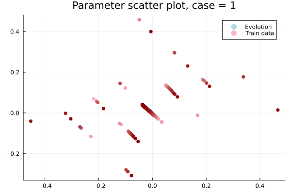
Learning smooth latent space trajectories
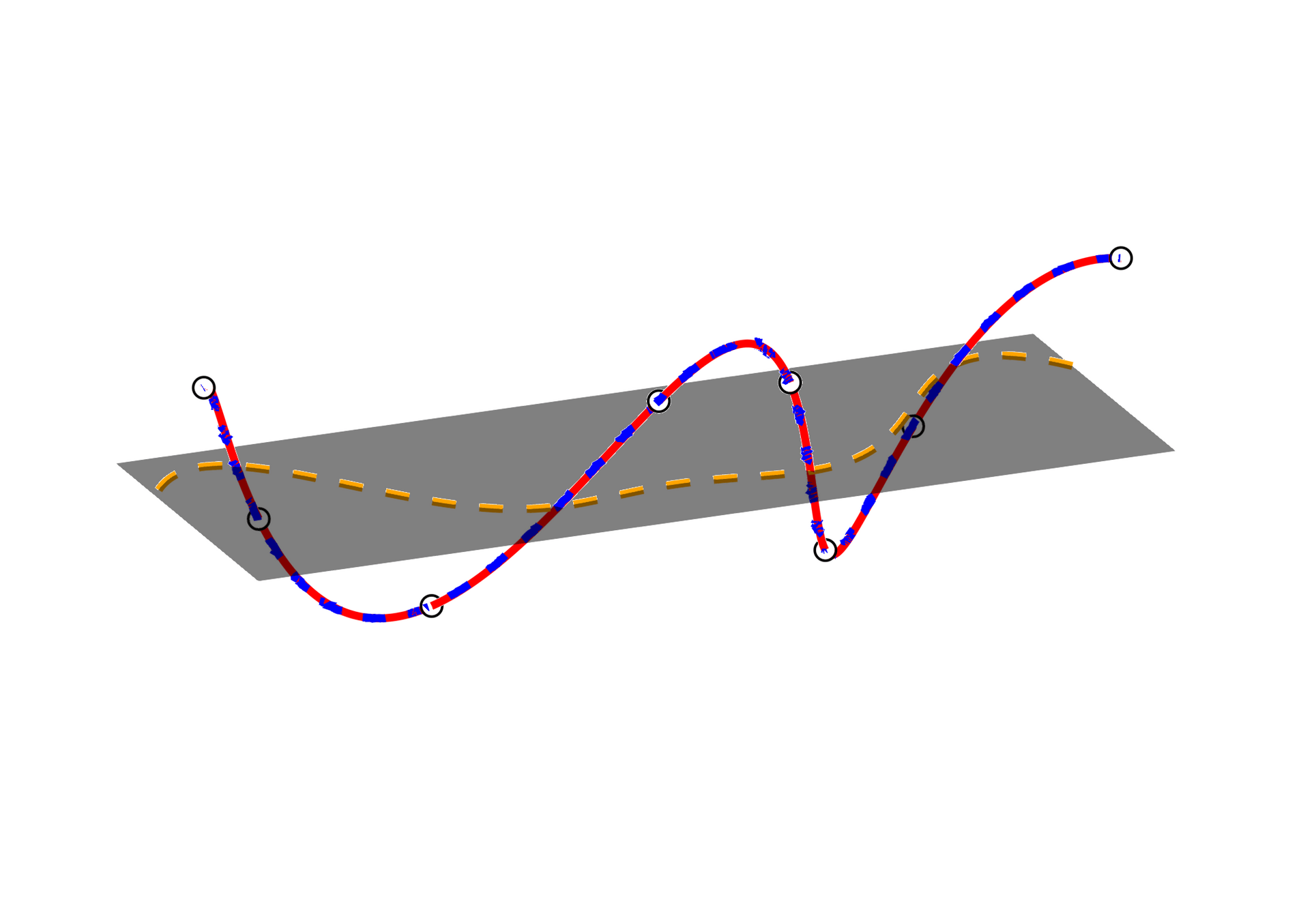
\(\text{Autoencoder ROM}\)
\(\text{SNF-ROM}\)
Evolution of ROM states
No deviation
SNF-ROM ensures accurate online dynamics evaluation.
Accurate capture of dynamics
2
Full order model (FOM)
Linear POD-ROM
Nonlinear ROM
Learn low-order spatial representations
Time-evolution of reduced representation with Galerkin projection
3
Autoencoder ROMs see a sharp rise in error due to deviation of the reduced states from the learned manifold.
Encoder-free ROMs have disjoint latent space representations which inhibit online evaluations.
Autoencoder ROMs
Auto-decoder ROMs
\(\text{Encoder}\)
\(\text{Decoder}\)
\(\text{Decoder}\)
\(\text{Loss }\)
\(\nabla_{\tilde{u}} L\)
4
\(\tilde{u}(t; \boldsymbol{\mu})\)
\(\Xi_\varrho\)
Q. What prior to place on the latent space to ensure smooth/accurate traversal?
Control the complexity of latent trajectories.
Supervised learning problem: \((\boldsymbol{x}, t; \boldsymbol{\mu}) \to \boldsymbol{u}(\boldsymbol{x}, t; \boldsymbol{\mu})\).
\(\text{Loss } (L)\)
\(\text{Backpropagation}\)
\(\nabla_\theta L\)
\(\nabla_\varrho L\)
\(\nabla_\theta L\)
\(\text{PDE Problem}\)
\((\boldsymbol{x}, t, \boldsymbol{\mu})\)
\(\text{ Parameters}\)
\( \text{and time}\)
\(\text{ Intrinsic ROM manifold}\)
\(\text{Coordinates}\)
\(\text{Smooth neural field MLP }(g_\theta)\)
\(\tilde{u}\)
\(\boldsymbol{x}\)
\(\boldsymbol{u}\left( \boldsymbol{x}, t; \boldsymbol{\mu} \right)\)
Learn \((t; \boldsymbol{\mu}) \to \tilde{u}(t; \boldsymbol{\mu})\) directly
5
Derivative calculation is carried out with automatic differentiation making the dynamics evaluation non-intrusive.
SNF-ROM with Lipschitz regularization (SNFL-ROM)
\(\text{Penalize the \textcolor{blue}{Lipschitz constant} of the MLP [arXiv:2202.08345]}\)
\(\text{[enwiki:1230354413]}\)
SNF-ROM with Weight regularization (SNFW-ROM)
\(\text{Directly penalize \textcolor{red}{high-frequency components} in }\dfrac{\text{d}}{\text{d} x}\text{NN}_\theta(x)\)
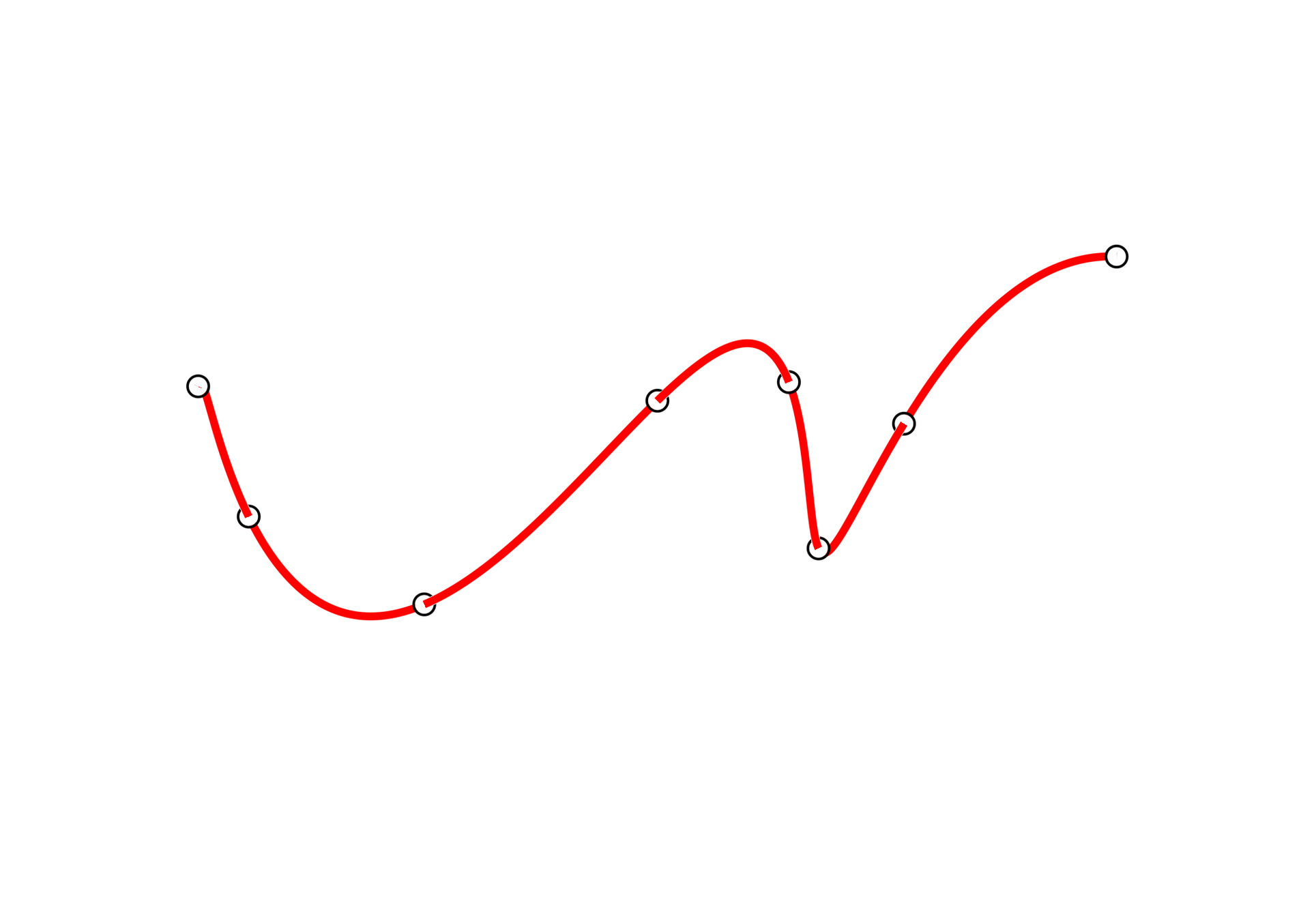
We present two approaches to learn inherently smooth and accurately differentiable neural field MLPs.
\({x}\)
\({u(x)}\)
Neural field MLPs are
non-differentiable
High freq. noise
8
Both Lipschitz regularization (SNFL) and weight regularization (SNFW) capture the 4-th order derivative accurately.
\(\text{Relative error } (\Delta t = \Delta t_0)\)
\(\text{Relative error } (\Delta t = 10\Delta t_0)\)
Oscillations due to variation in projection error
Highly diffusive; even POD with 2 modes
6
\(\text{CAE-ROM}\)
\(\text{SNFL-ROM}\)
\(\text{SNFW-ROM}\)
SNFL-ROM, SNFW-ROM effectively capture the traveling shock.
7
\(\text{CAE-ROM}\)
\(\text{SNFL-ROM}\)
\(\text{SNFW-ROM}\)
CAE-ROM has complex diverging trajectories, where as SNF-ROM has near linear and easy to follow ones
Online dynamics solve matches learned trajectories
Online evaluation deviates!
Distribution of reduced states \((\tilde{u})\)
By Vedant Puri
Presented at WCCM 2024


