


Vedant Puri
PhD student at Carnegie Mellon University
Vedant Puri
https://vpuri3.github.io/
MAY 04, 2026
1
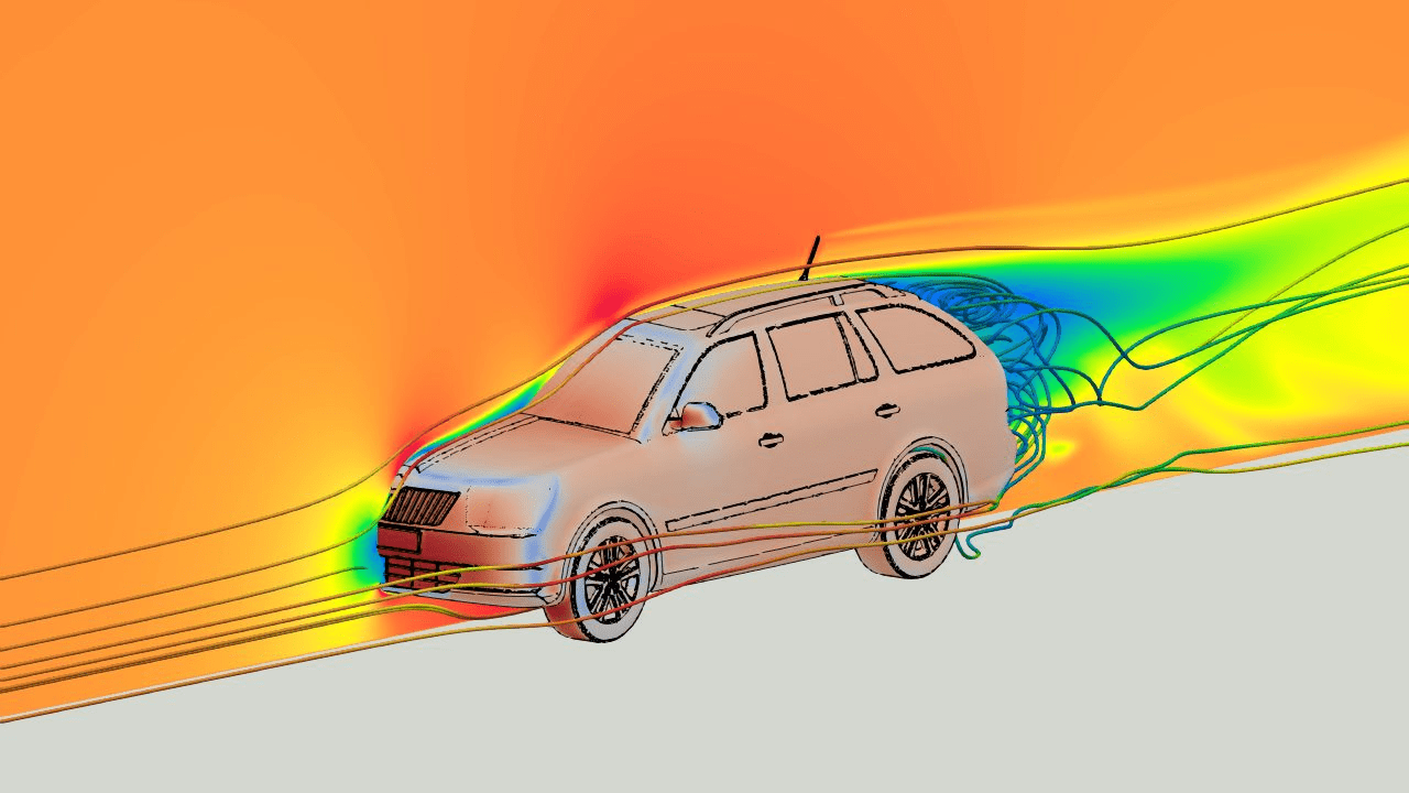
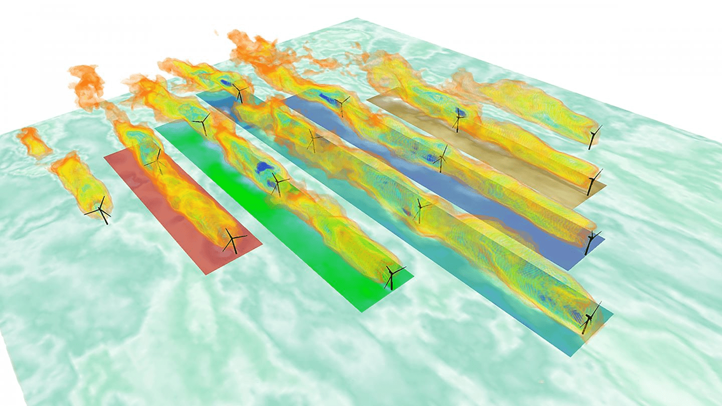
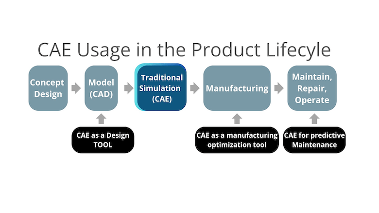
Predictive maintenance
Design space exploration
[2]
[1]
[3]
[1] CFD Direct / OpenFOAM – “OpenFOAM HPC on AWS with EFA”, cfd.direct
[2] EurekAlert — “New concrete system may reduce wind-turbine costs”
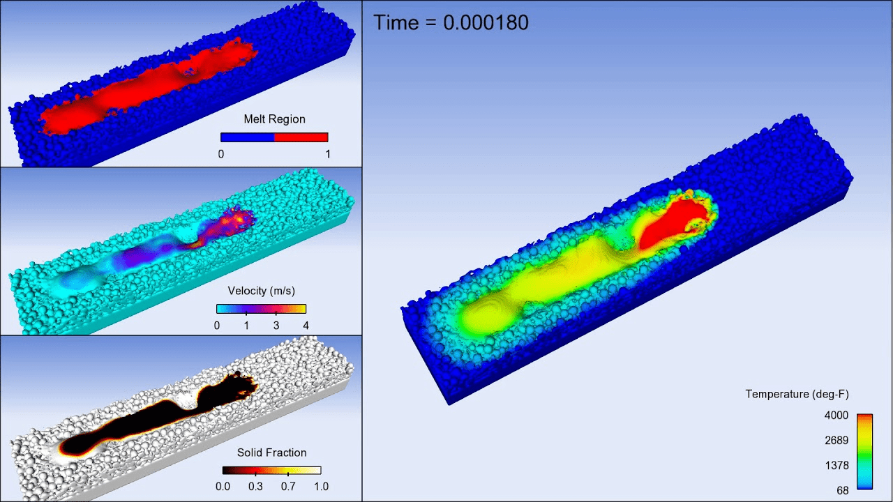
[3] Flow-3D, “FLOW-3D AM” product page, flow3d.com
Process optimization
[1]
2
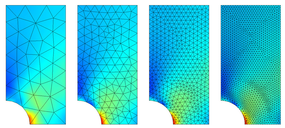
[1] COMSOL — “Mesh Refinement”
[2] Langtangen, H. P. — INF5620: Finite Element Methods (Lecture Notes)
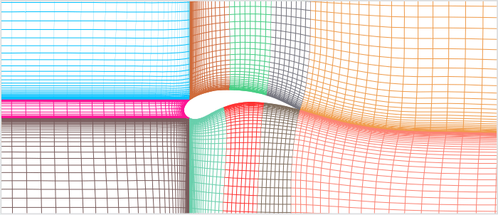
[3] GridPro Blog — “The Art and Science of Meshing Airfoil”
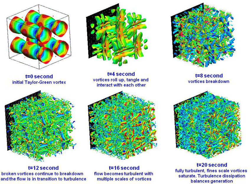
[4] ResearchGate — “Transition to turbulence of Taylor-Green Vortex at different time (DNS)” (figure)
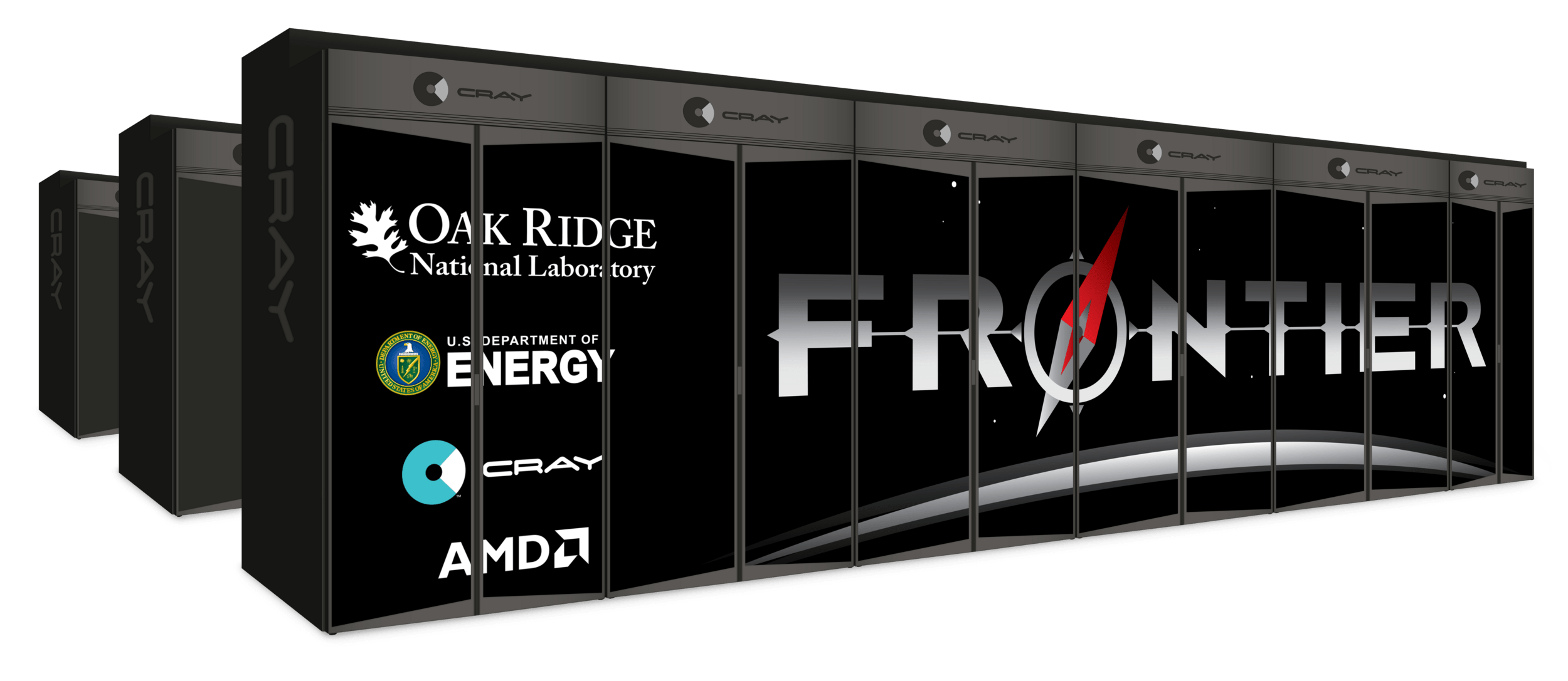
[5] ORNL / U.S. Department of Energy — “DOE and Cray deliver record-setting Frontier supercomputer at ORNL”
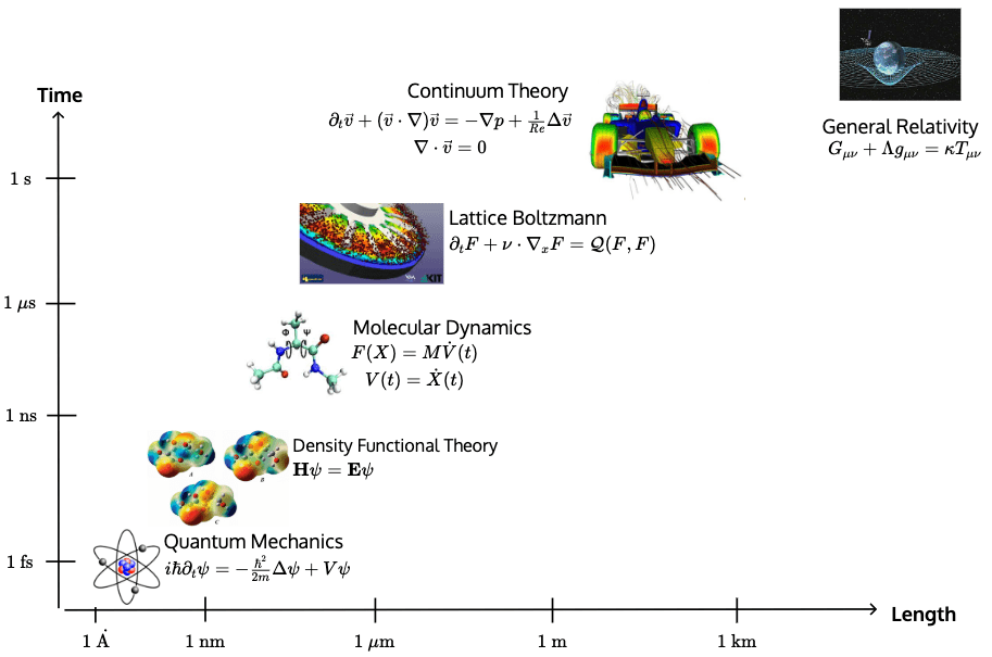
Governing Equations
[1]
[2]
Discretization machinery
Repeated large system solves
[5]
Multiscale physics \(\implies\) small \(\Delta t\)
[4]
Complex geometry \(\implies\) fine meshes
[3]
Complex geometry \(\implies\) fine meshes
The cost of this procedure scales poorly for several reasons.
3
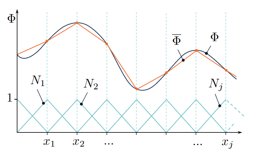
(Explicit) Weighted sum of polynomial interpolants
[1]
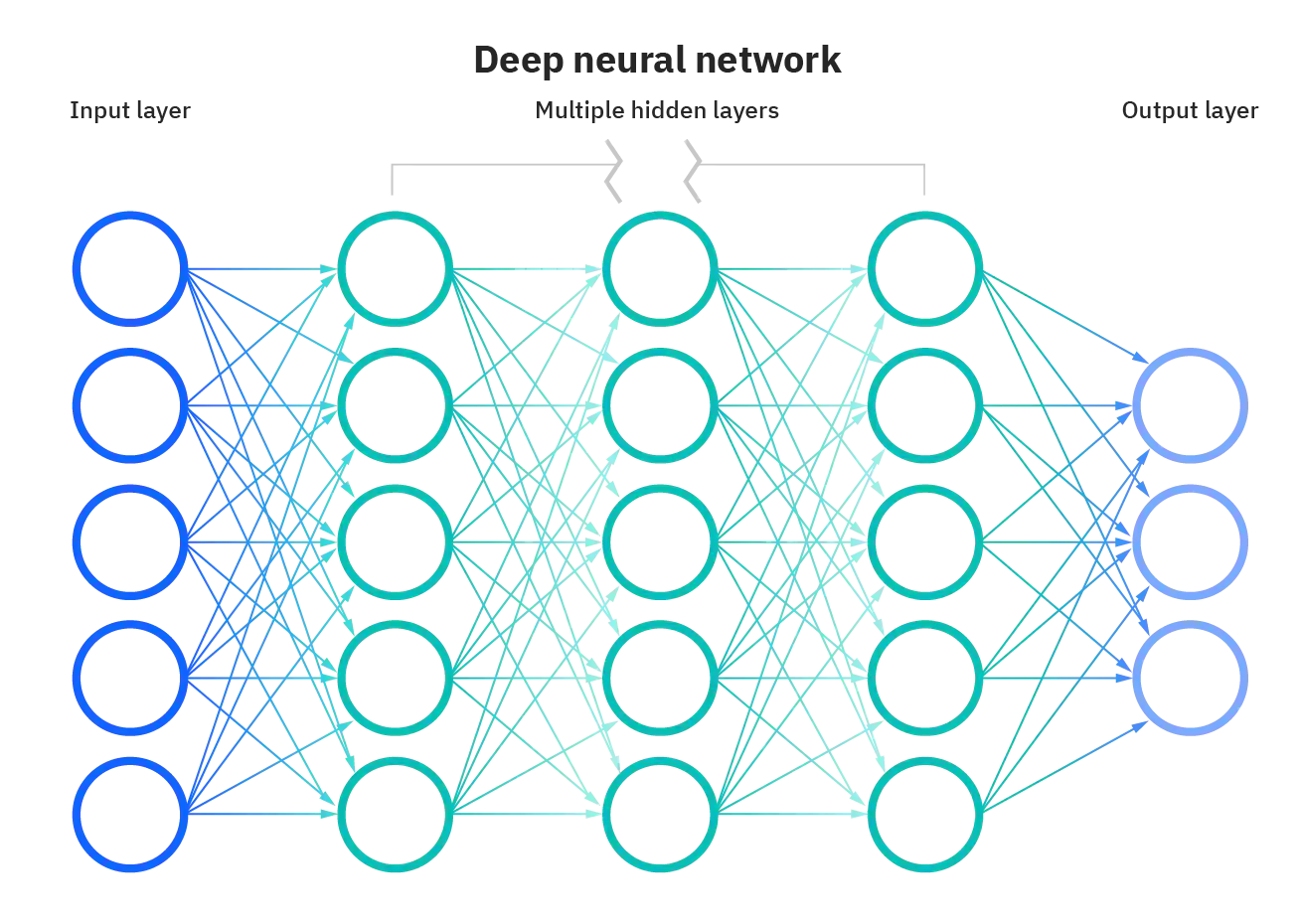
(Implicit) High-dim nonlinear feature learners
[2]
Cannot learn from data
Can learn from data
Large cost per simulation
Cheap evaluation after training
High-accuracy
Problem-specific
Robust
Up to \(0.1\%\) accuracy
[1] Math StackExchange — “Interpolation in Finite Element Method”
[2] ResearchGate — “Structure of a Deep Neural Network” (figure)
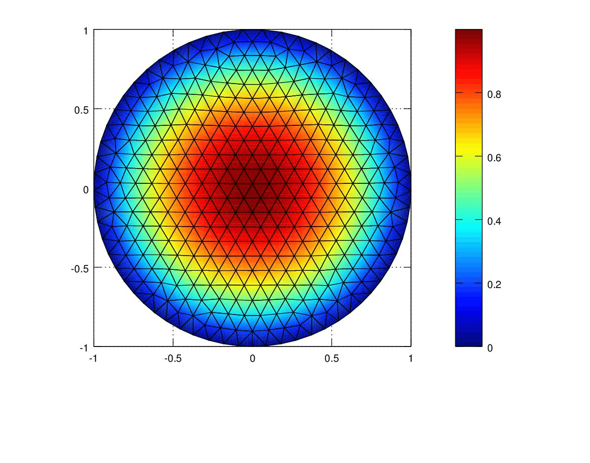
\(\text{Mesh ansatz}\)
\({u}(x)=\)
\(u(x) = \)
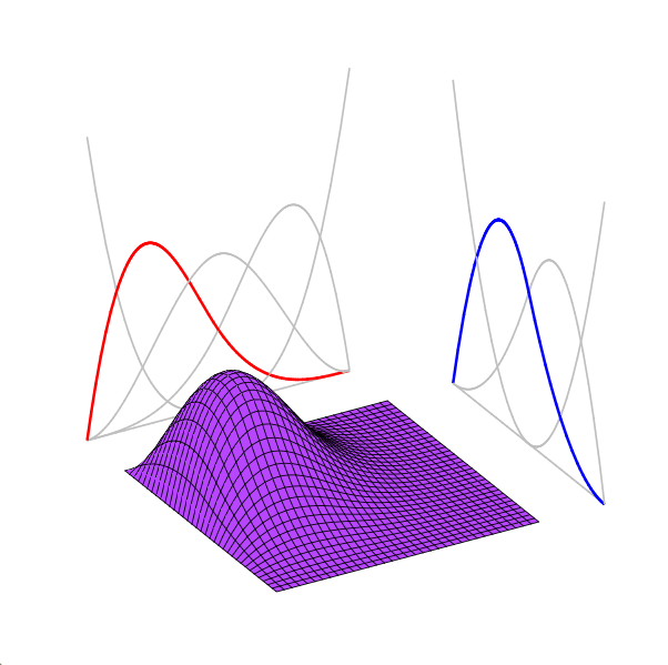
\(\text{Neural ansatz}\)
\(\text{Physics-based}\)
\(\text{Data-driven}\)
\(\text{Numerical}\)
\(\text{Simulation}\)
\(\text{Reduced Order}\)
\(\text{Modeling}\)
\(\text{Neural ROMs}\)
\(\text{Surrogate}\)
\(\text{Learning}\)
\(\text{Transformers}\)
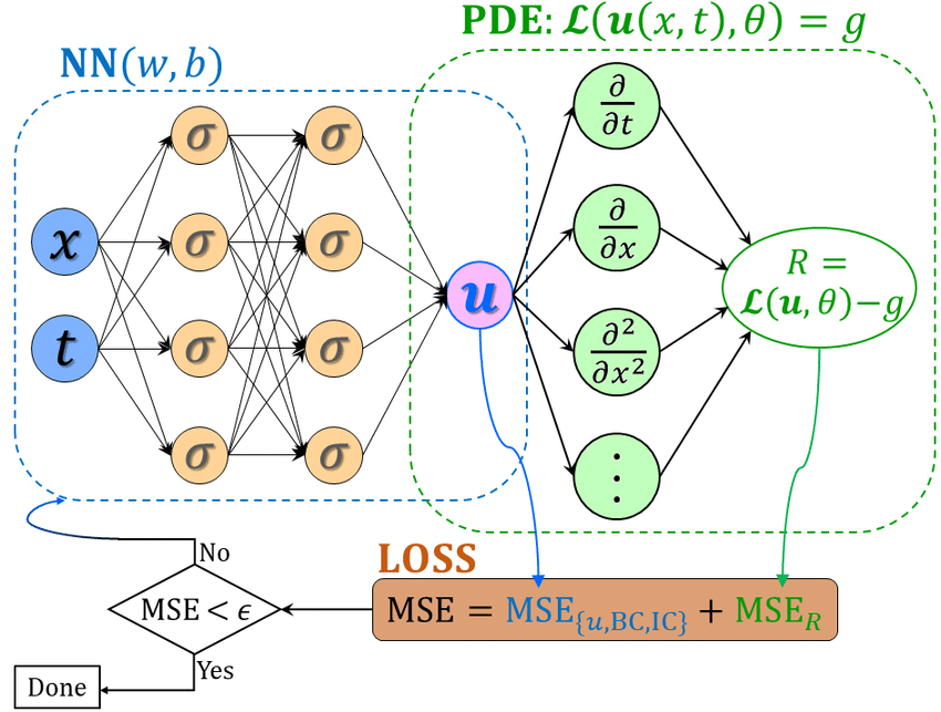
\(\text{PINNs}\)
\(\text{Finite Elements}\)
\(\text{PCA/POD}\)
\(\text{Graph Networks}\)
4
Scalable transformer models for large-scale surrogate modeling
[1]
[3]
[2]
[1] CFD Direct / OpenFOAM — “Introduction to Computational Fluid Dynamics”
[2] ResearchGate — “Schematic of a Vanilla Physics-Informed Neural Network” (figure)
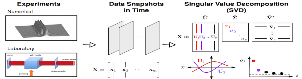
[3] Kutz, J. N. — “Data-Driven Modeling & Dynamical Systems” (UW)
5
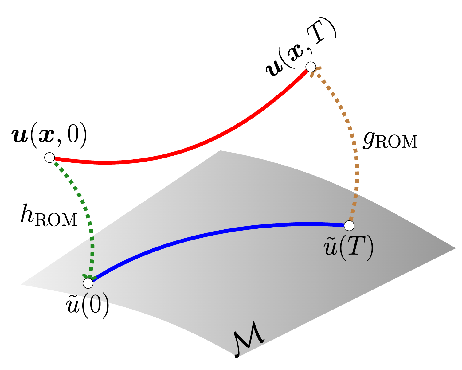
Large training cost is amortized over several evaluations
Model learns to predict \(\boldsymbol{u}\) over a distribution of \(\boldsymbol{\mu}\)
6
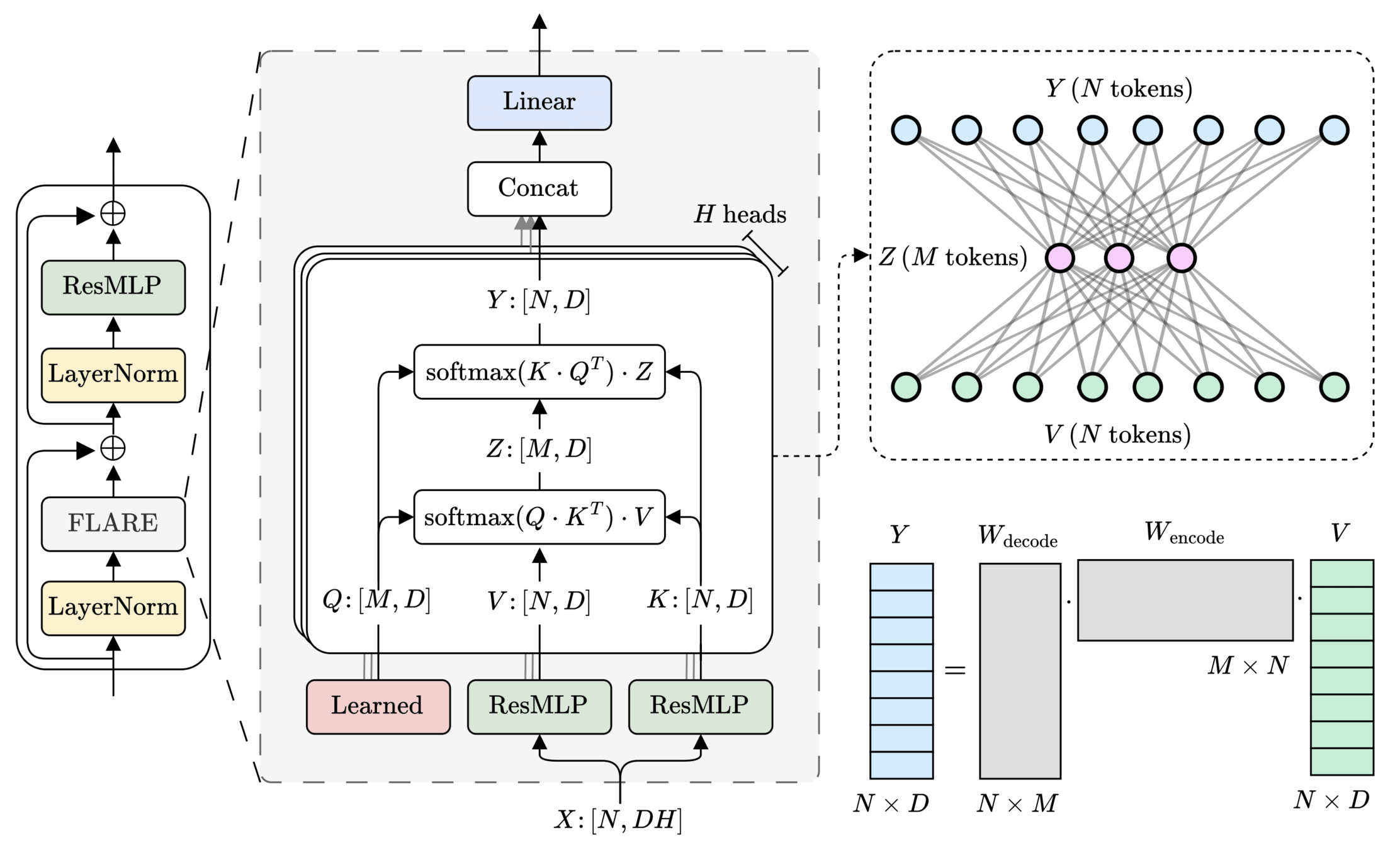
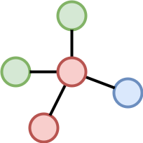
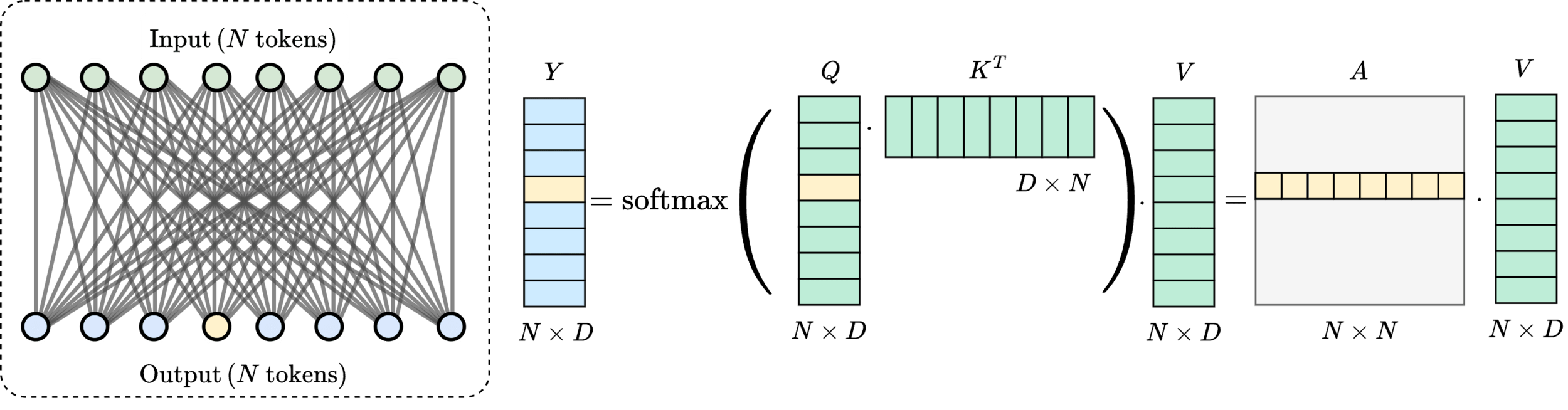
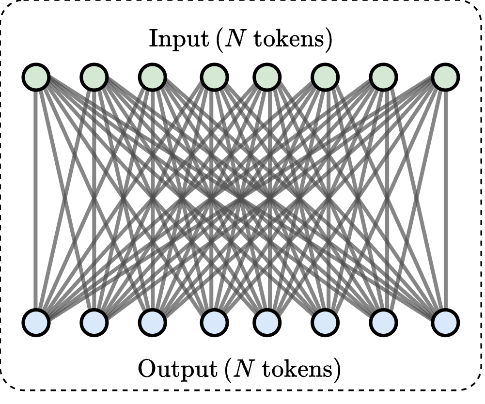
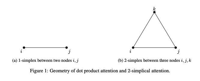
Message-passing on a dynamic all-to-all graph.
[1] Vaswani et al. — “Attention Is All You Need”, NeurIPS 2017
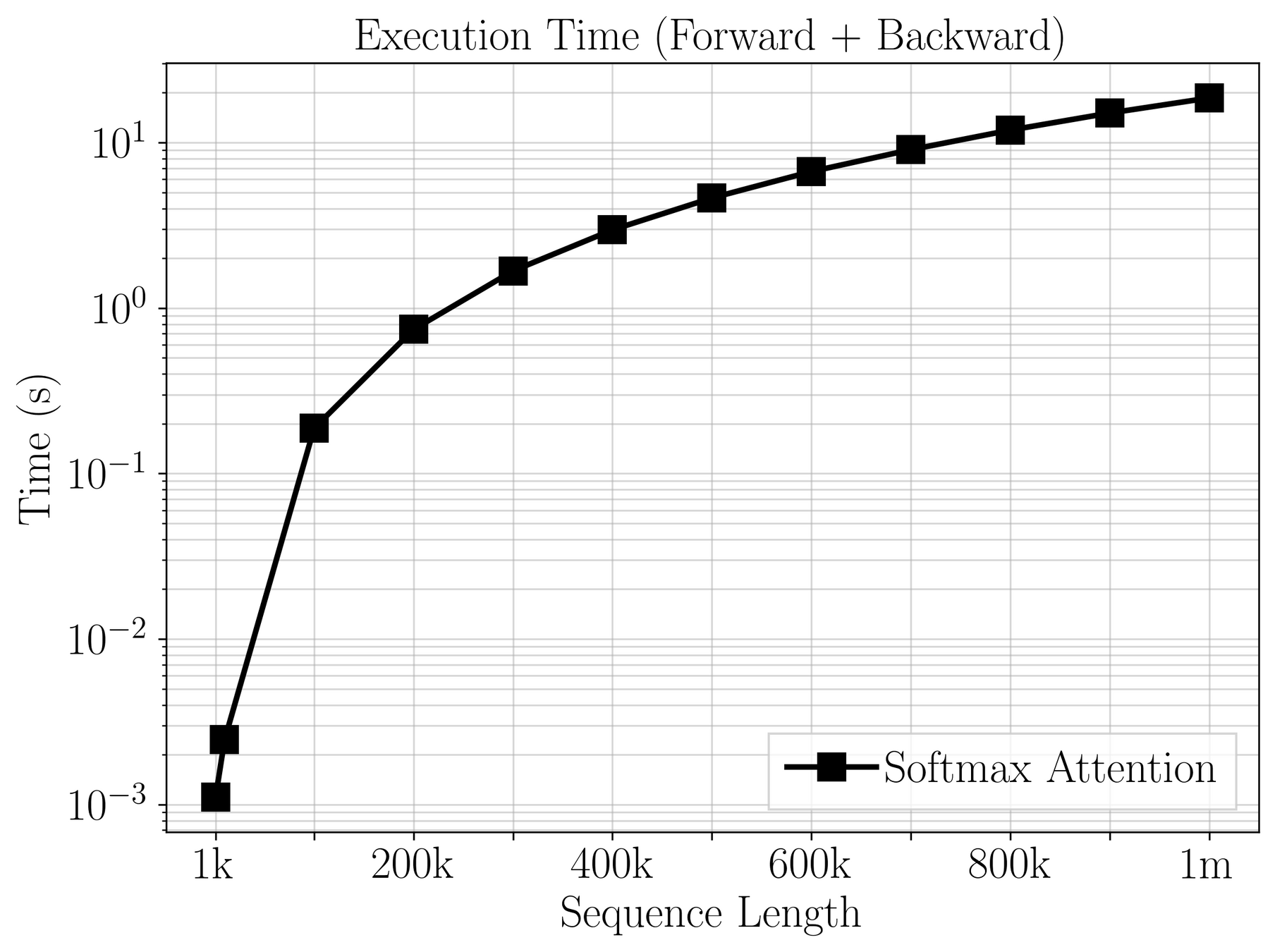
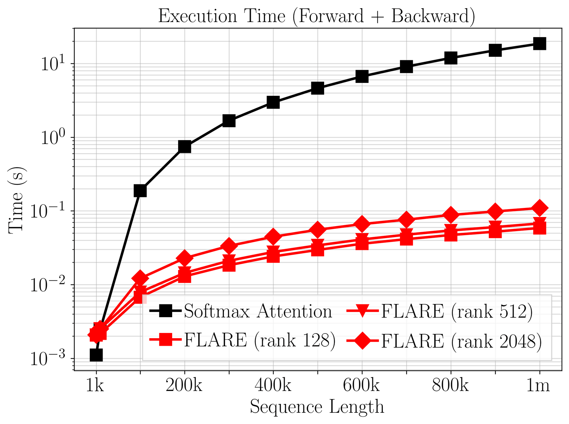
Quadratic (\(\mathcal{O}(N^2)\)) cost limits scalability
7
Over \(20~\text{s}\) per gradient step on a mesh of 1m poins!
Goal: enable transformer models on large meshes.
[1] Vaswani et al. — “Attention Is All You Need”, NeurIPS 2017
\([1]\)
8
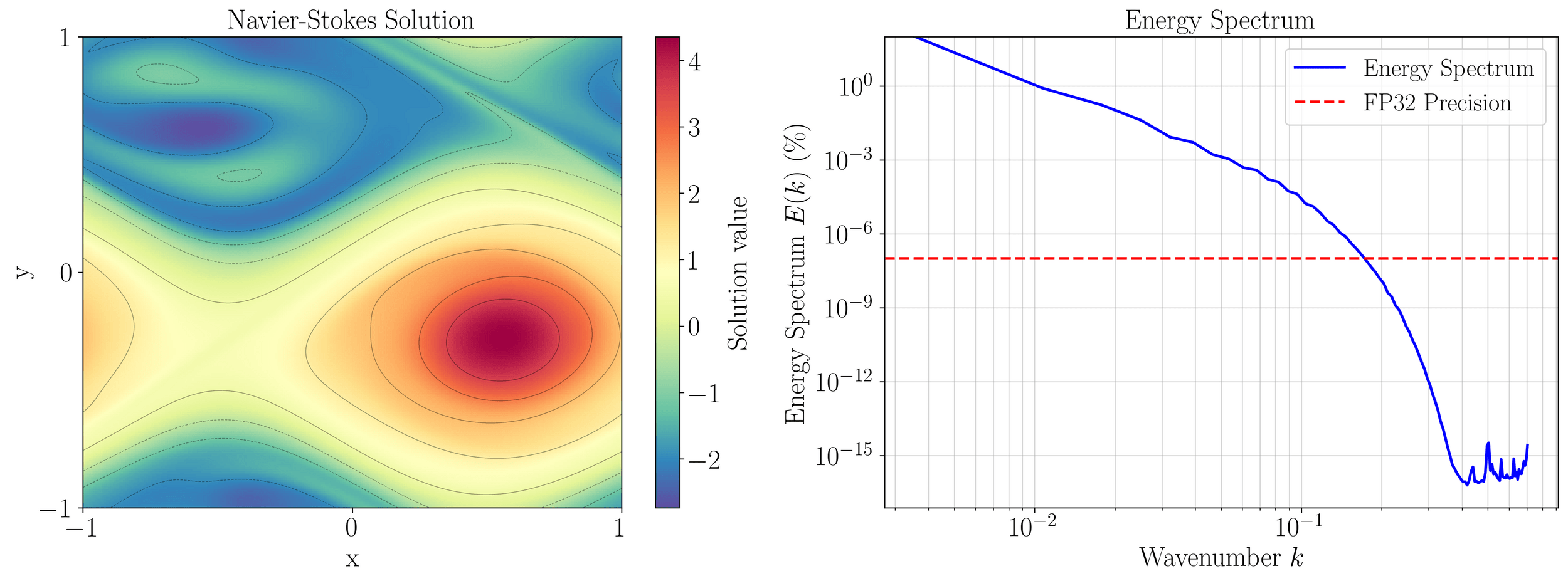
Solution operator requires global communication.
Forward operator is implemented with sparse, structured communication.
Need principled strategy for reducing communication cost.
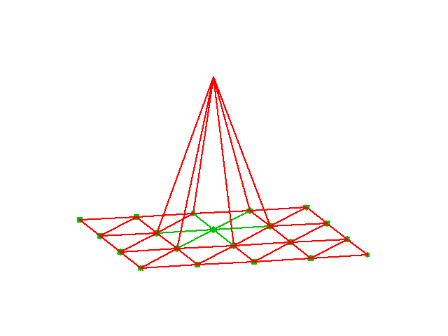
Detour: finite elements
[1] ParticleInCell.com — “Finite Element Experiments in MATLAB” (2012)
[1]
9
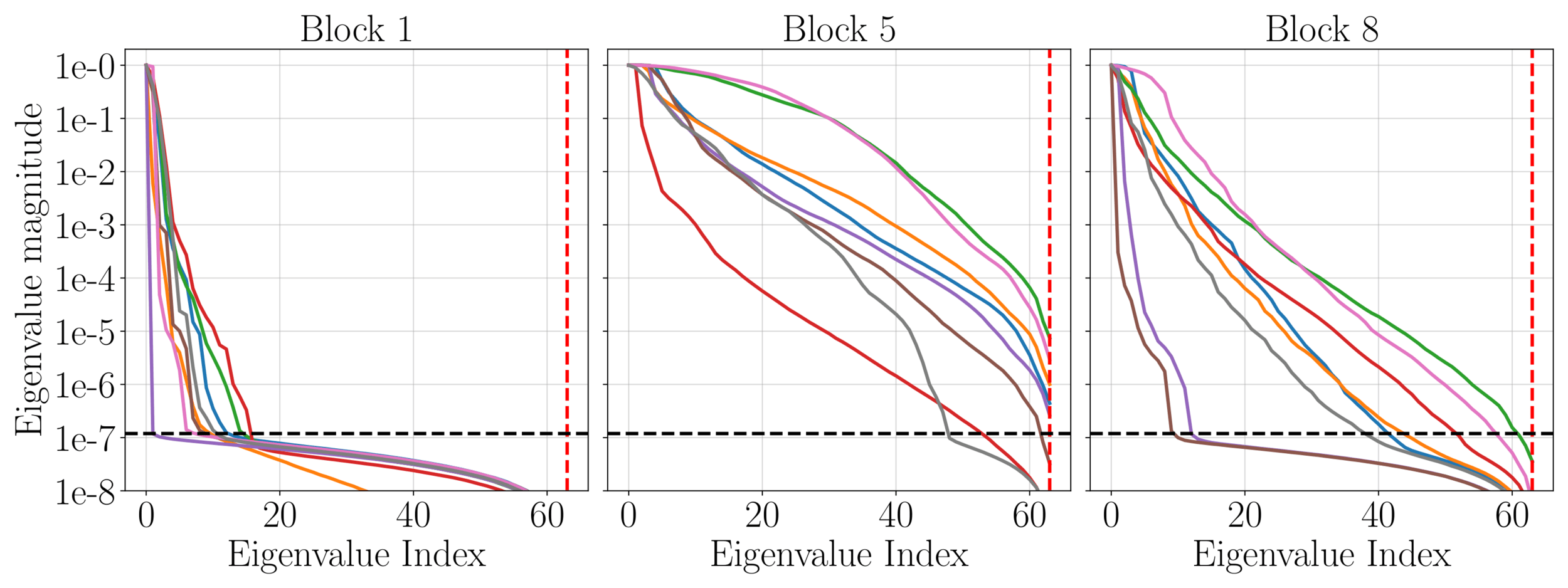
Smoothness implies redundancy in communication.
9
Smoothness implies redundancy in communication.
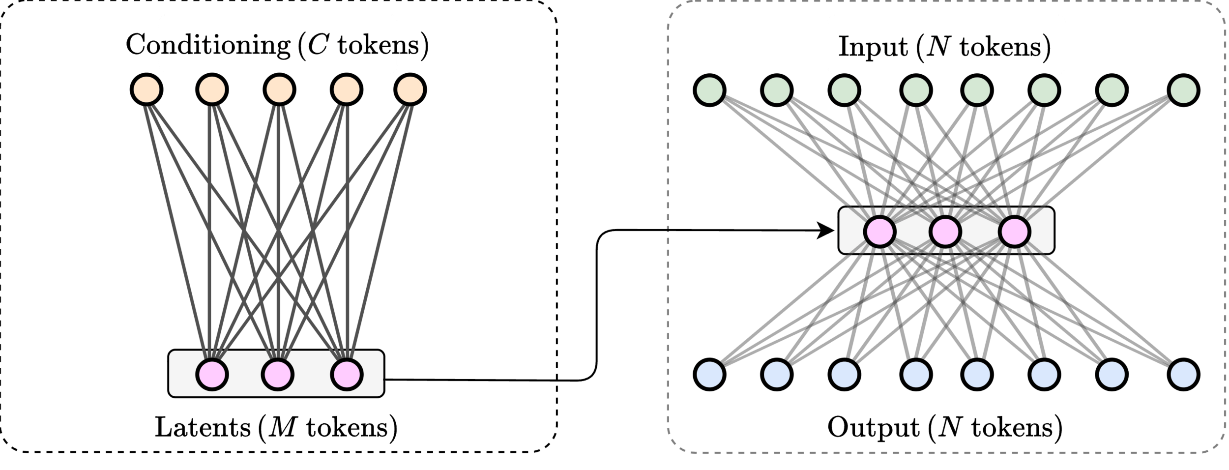
Method: club matching points to one cluster and communicate together.
10
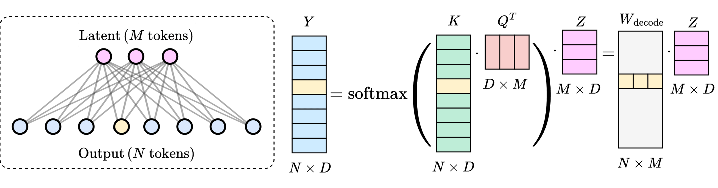
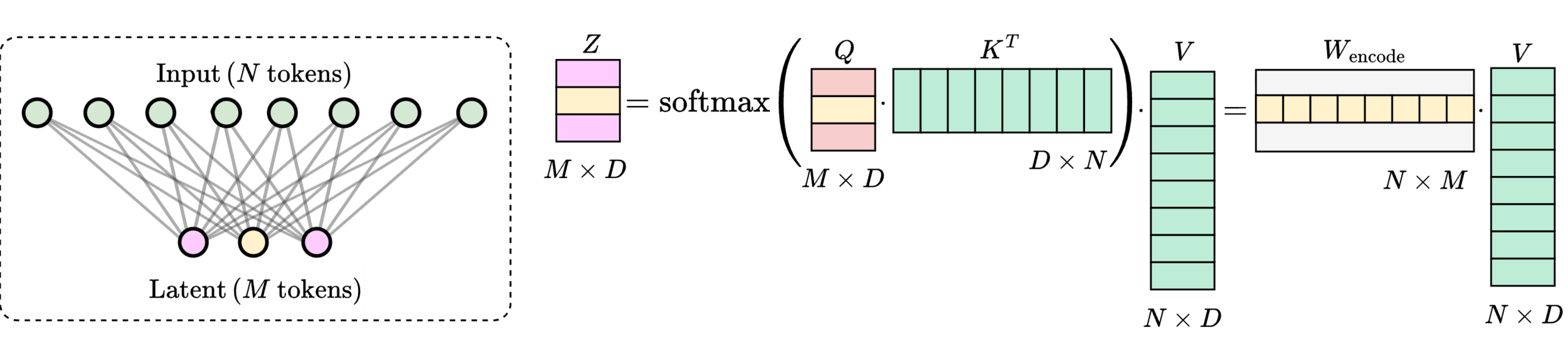
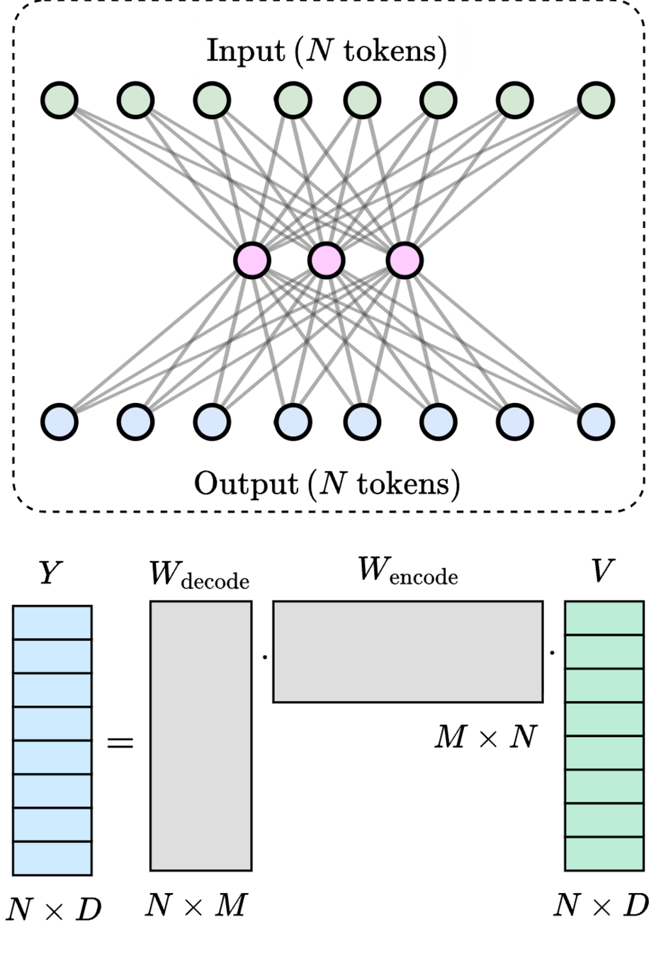
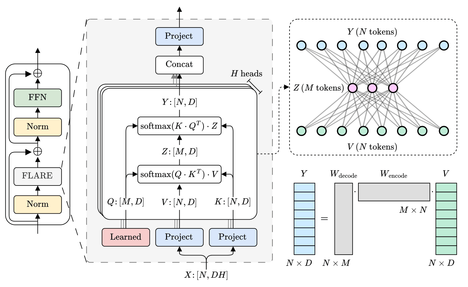
\(M\) learned queries
11
\(\mathcal{O}(2MN) \ll \mathcal{O}(N^2)\)
\(\text{rank}(W_\text{encode}\cdot W_\text{decode}) \leq M\)
\(>200\times\) speedup
\(\text{(} M \text{ tokens)}\)
\(\text{Latent}\)
[1] Vaswani et al. — “Attention Is All You Need”, NeurIPS 2017
\([1]\)
12
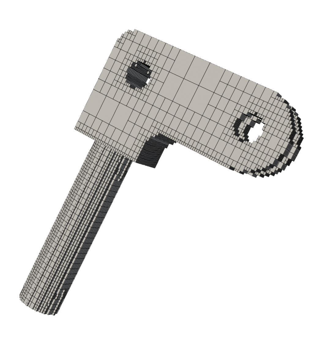
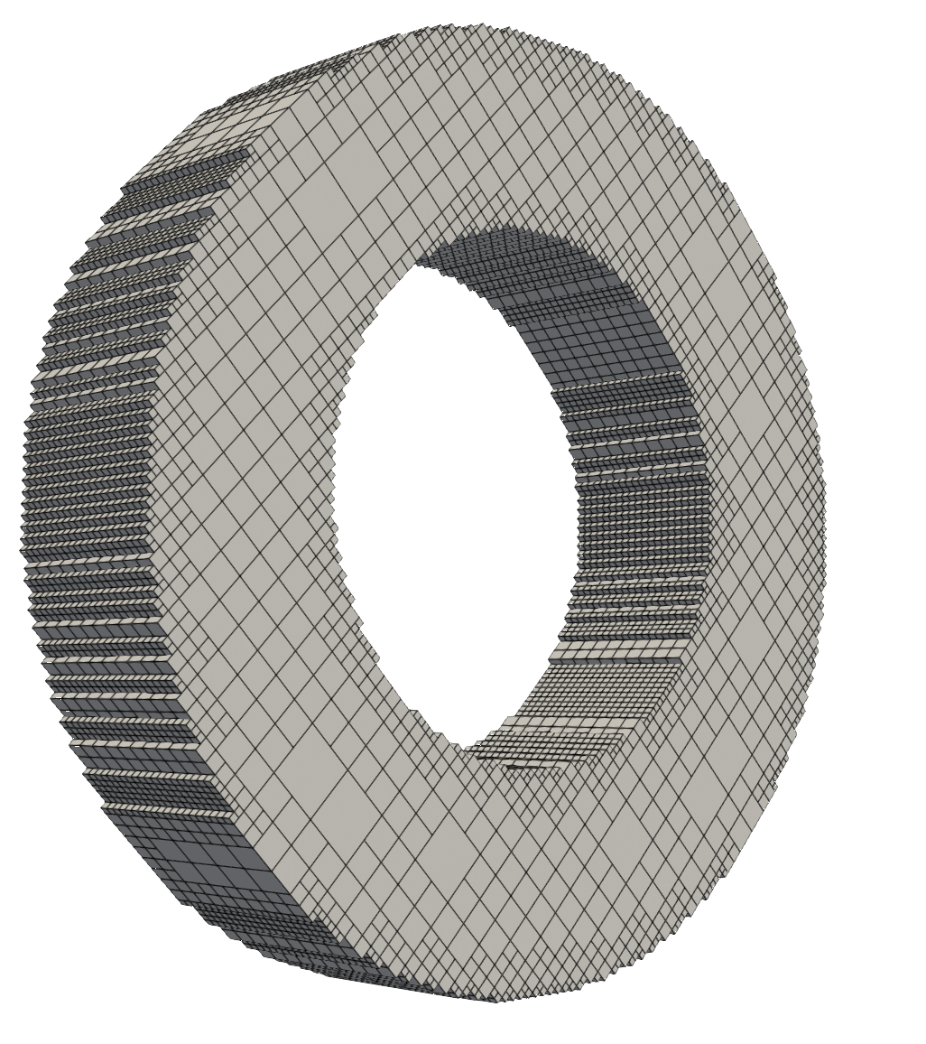
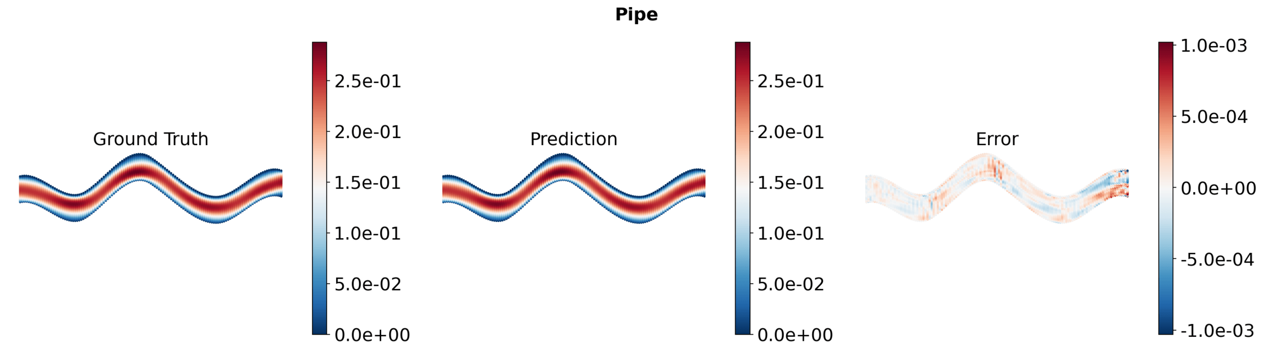
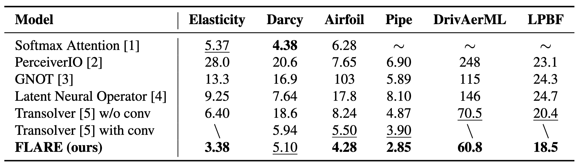
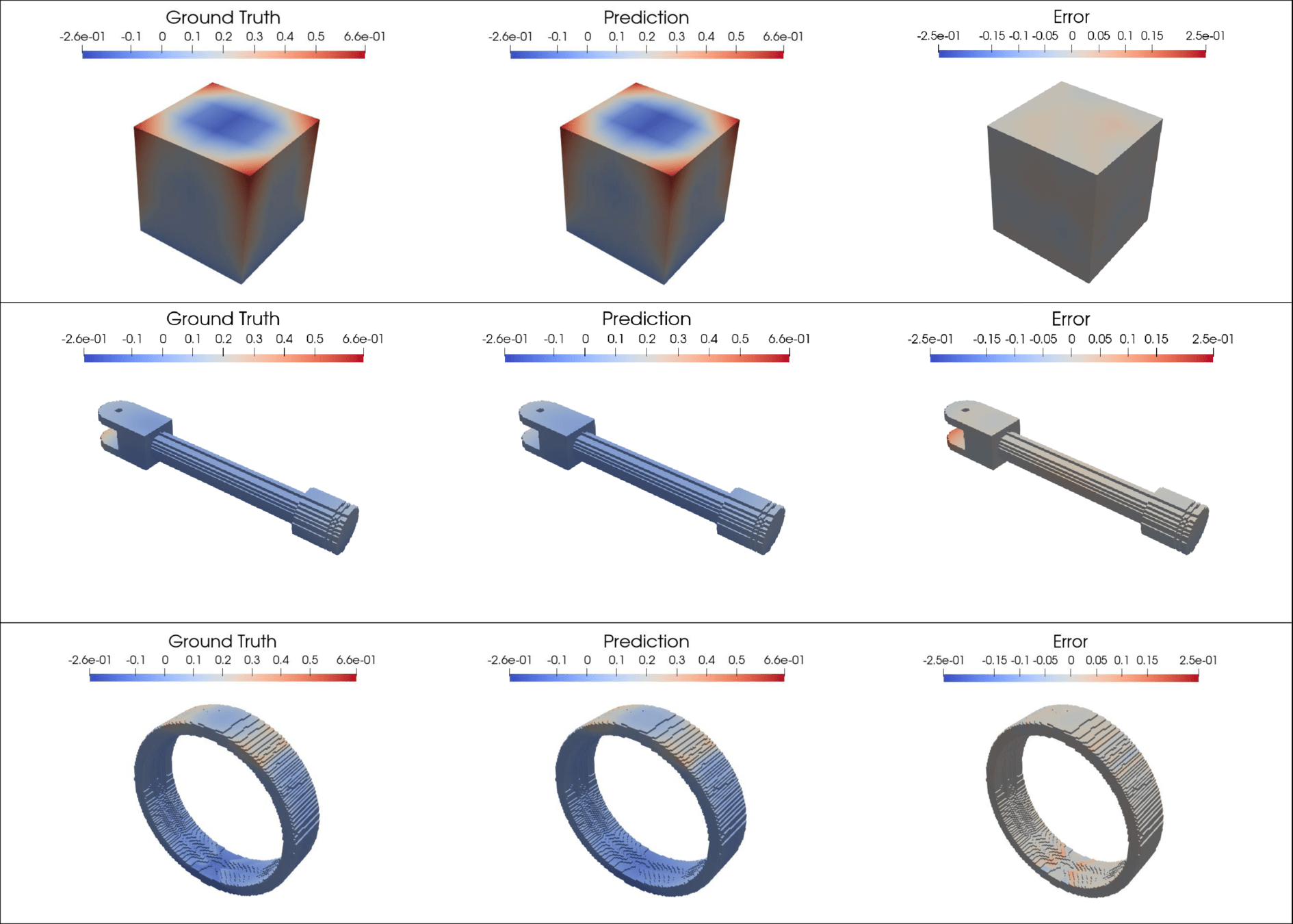
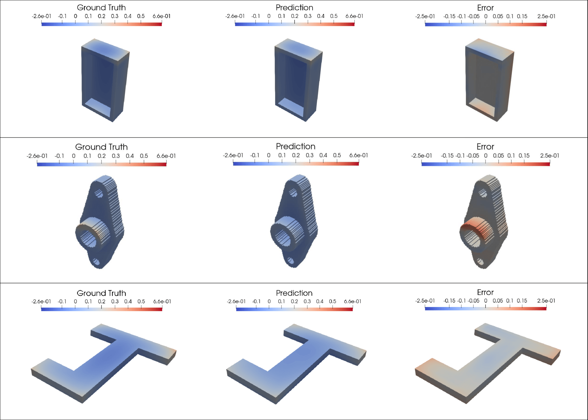
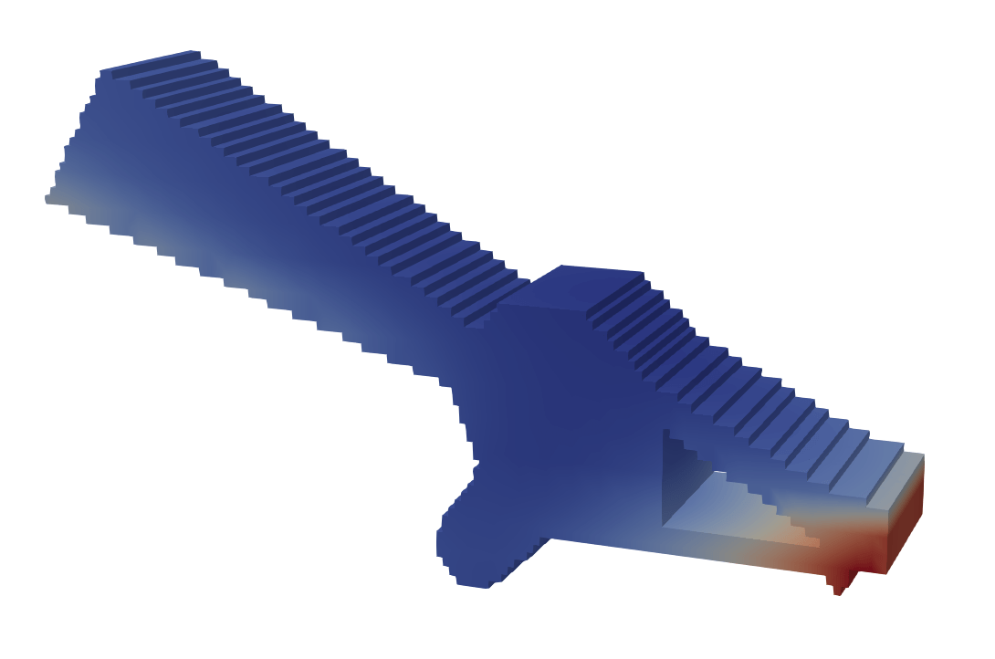
Pipe
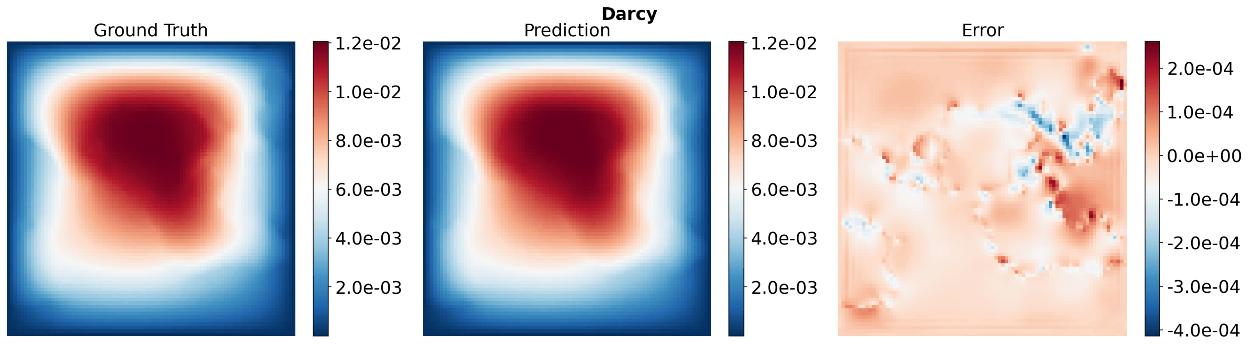
Darcy
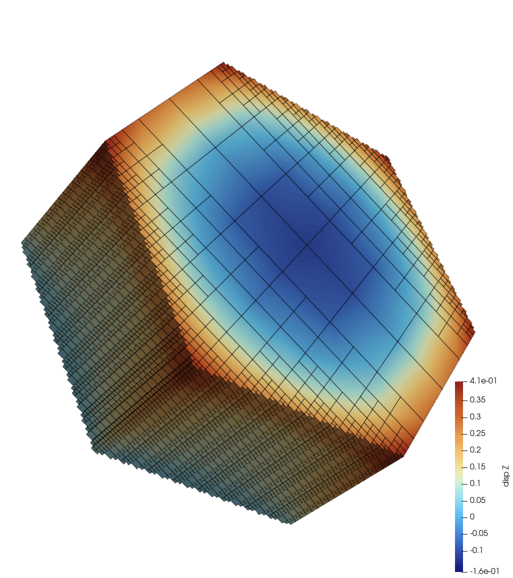
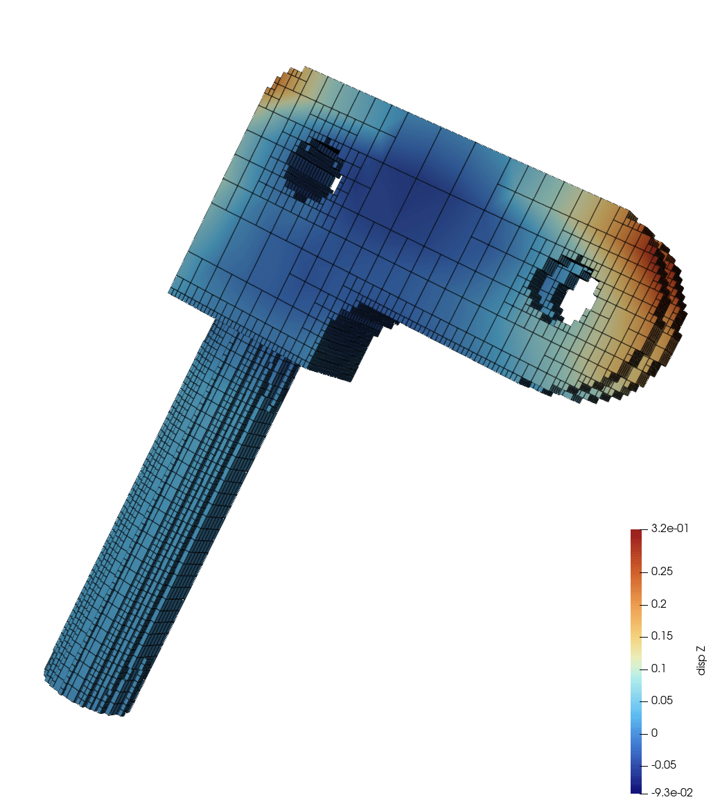
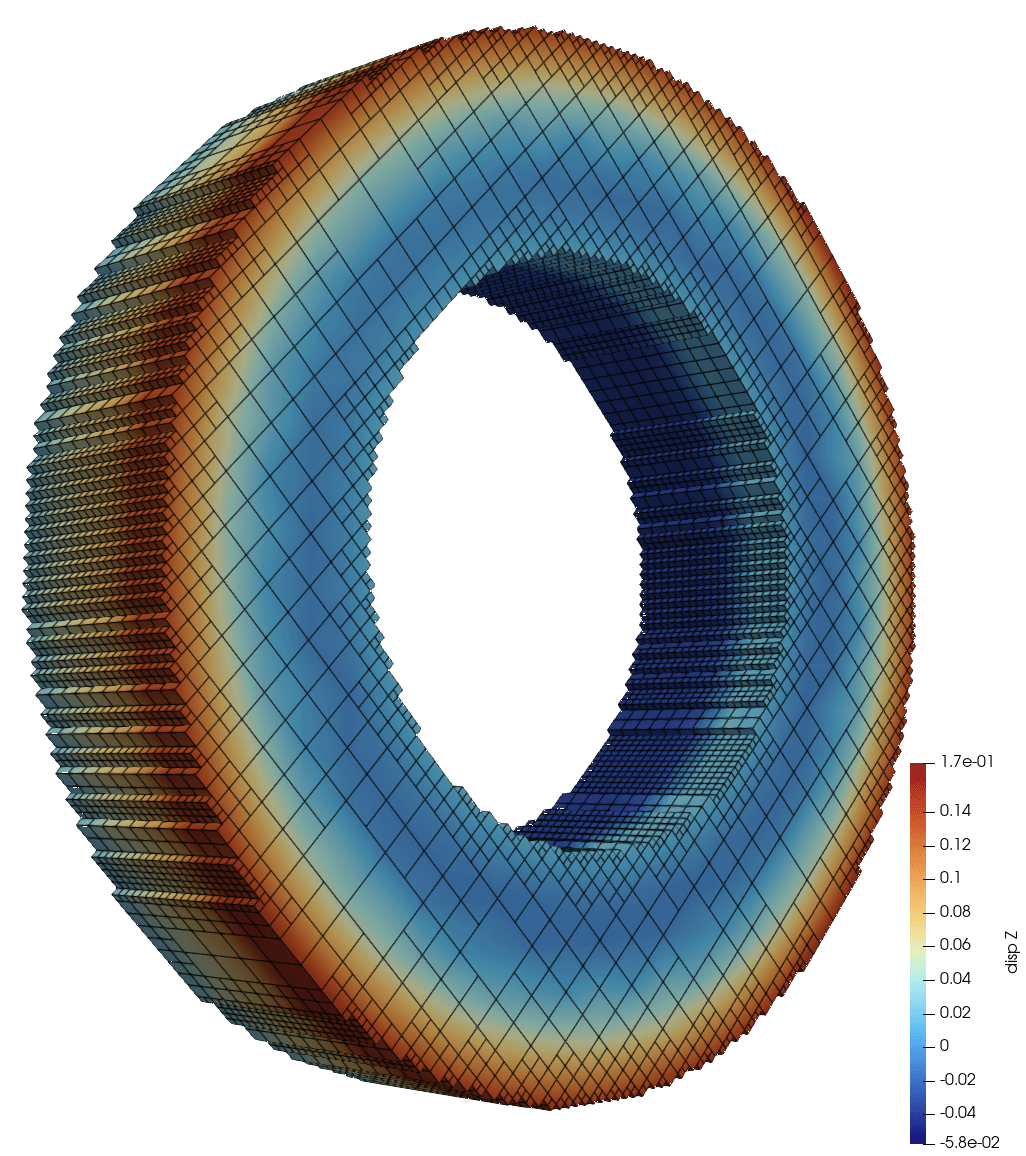
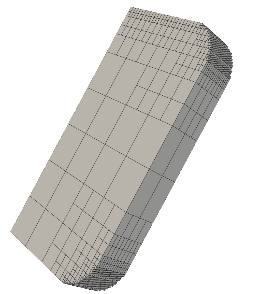
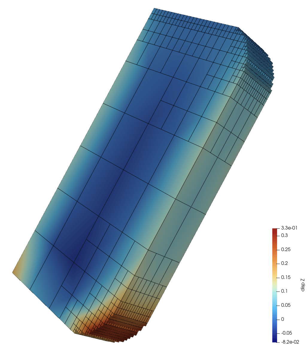
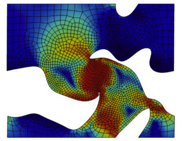
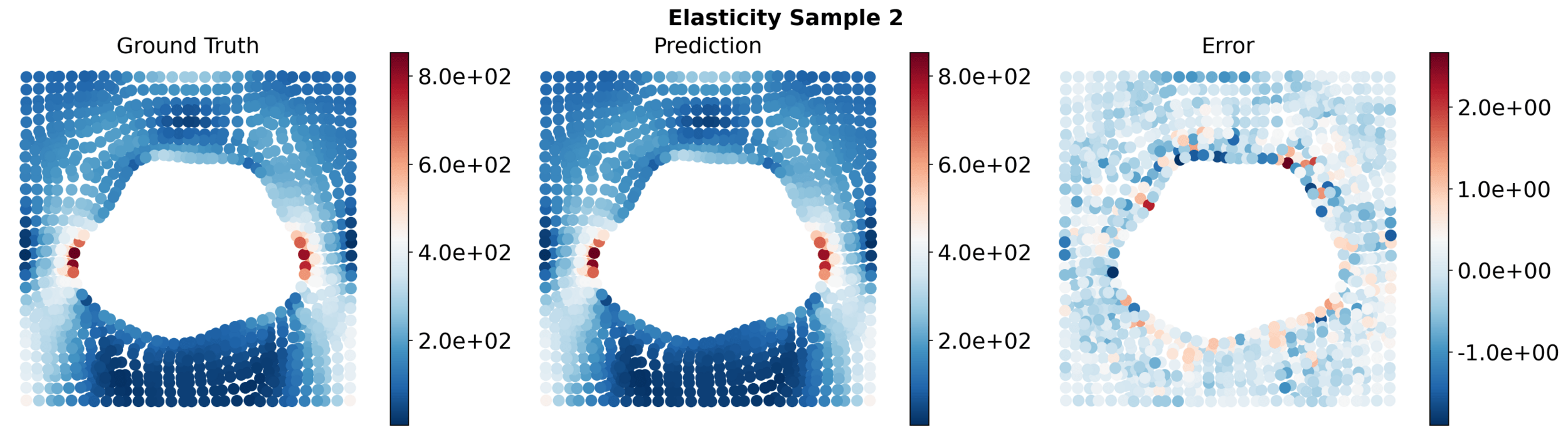
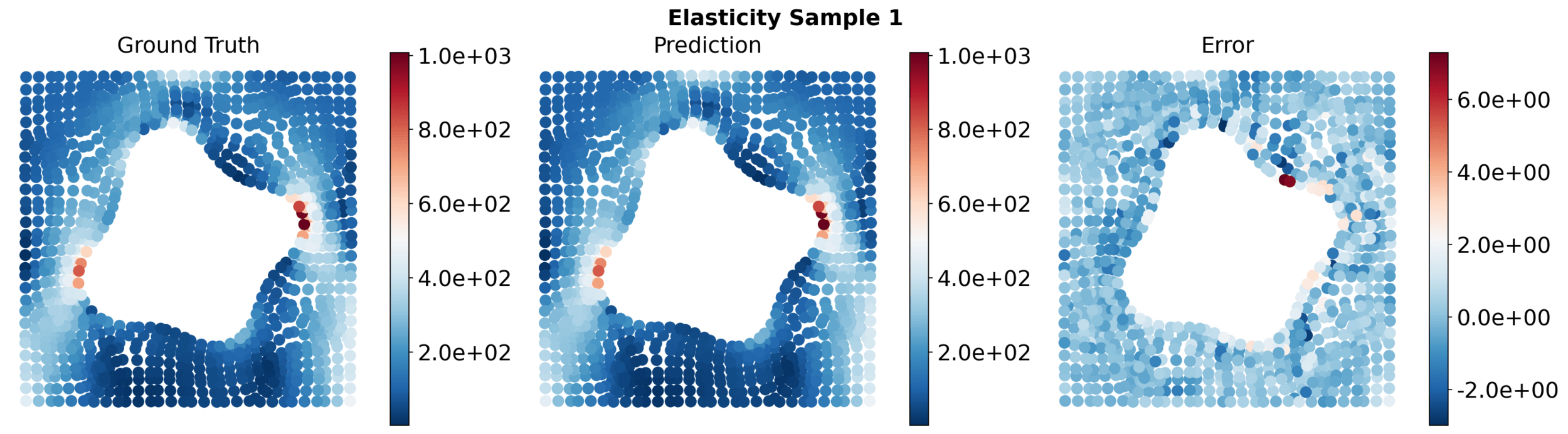
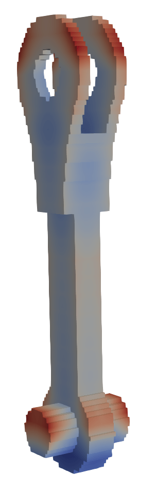
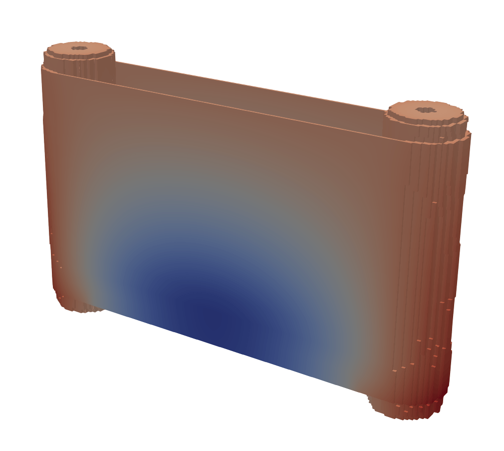
Elasticity
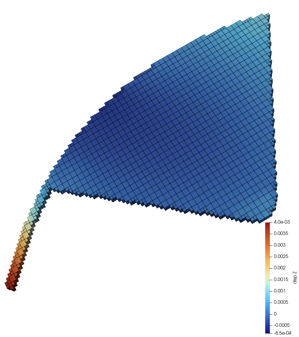
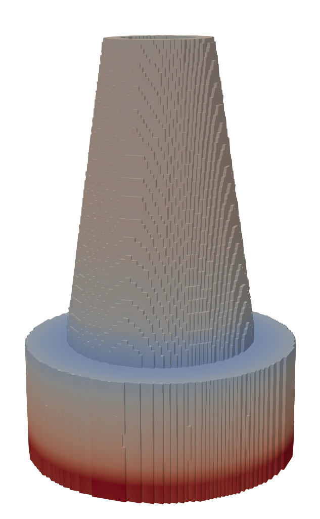
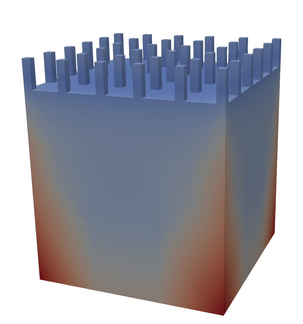
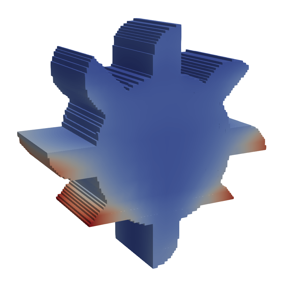
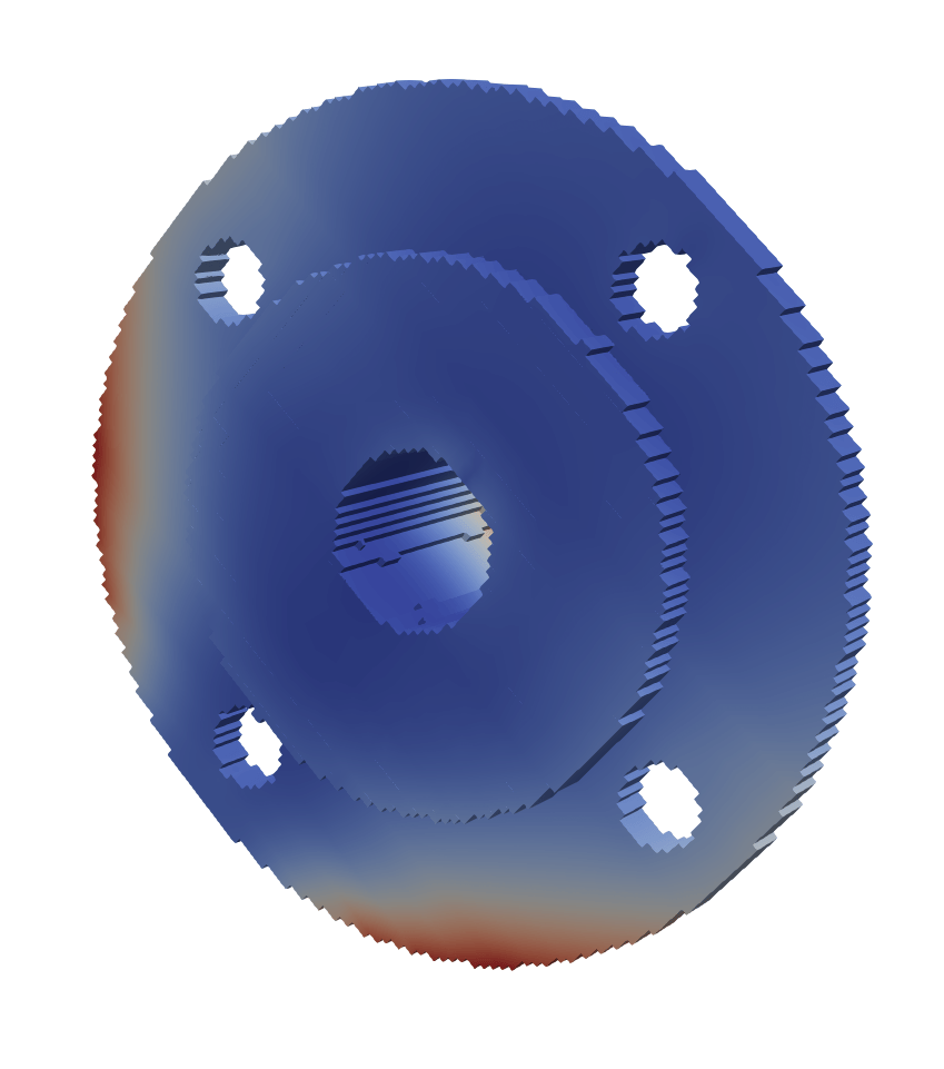
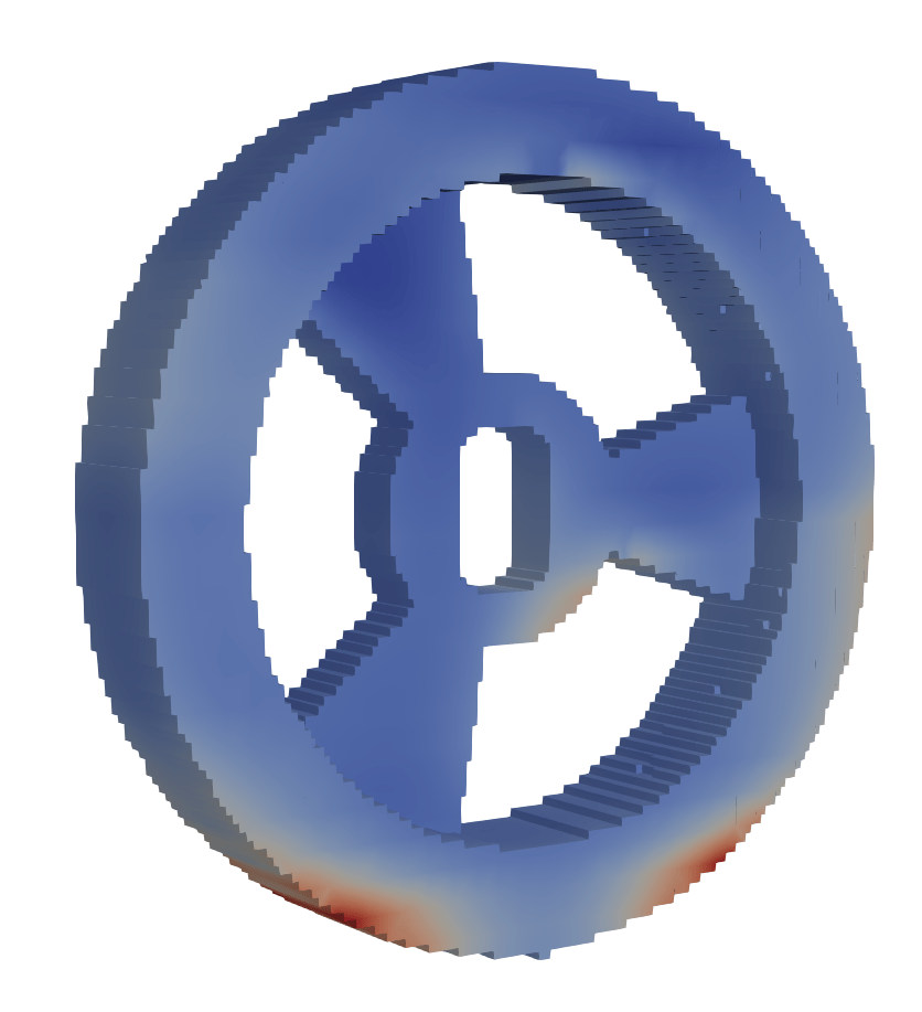
LPBF
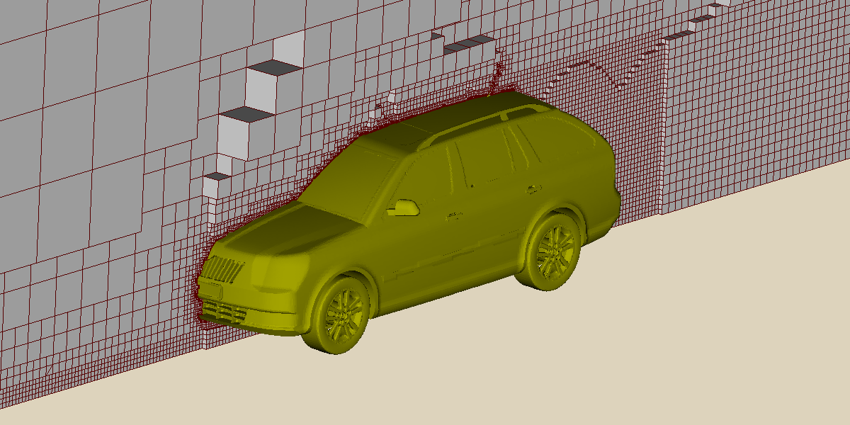
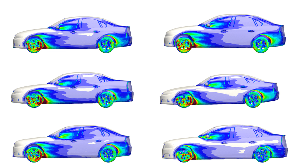
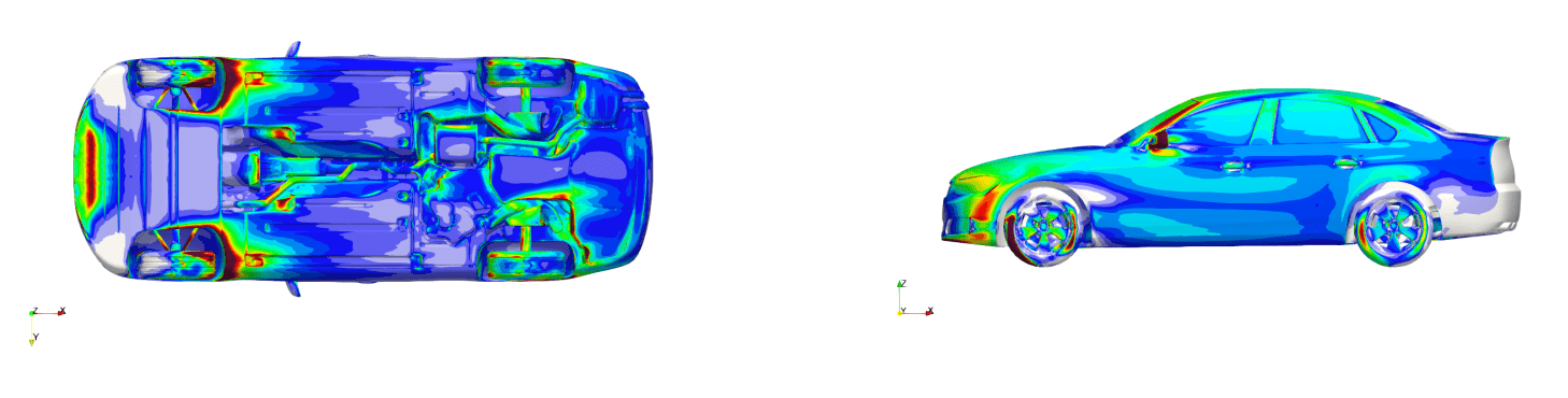
DrivAerML
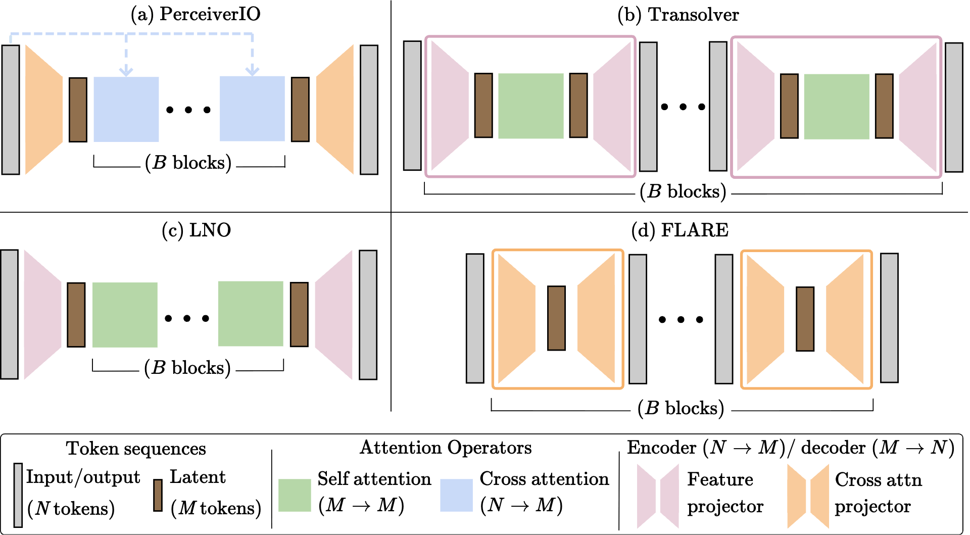
[1] Vaswani et al. — “Attention Is All You Need”, NeurIPS 2017
[2] Jaegle et al. — "PercieverIO: A General Architecture for Structured Inputs & Outputs", ICLR 2022
[3] Hao et al., — "GNOT: A General Neural Operator Transformer for Operator Learning", PMLR 2023
[4] Wang et al. —"Latent Neural Operator", NeurIPS 2024
[5] We et al. — "Transolver: A Fast Transformer Solver for PDEs on General Geometries", ICML 2024
13
14
15
16
import torch.nn.functional as F

def flare_multihead_mixer_inefficient(Q, K, V):
  	"""
    Args - Q: [H M D], K, V: [B H N D]
	Ret - Y: [B H N D]
	"""

	# [B H M N]
    scores = Q @ K. mT
    # [B H M N]
	W_encode = F.softmax(scores, dim = -1)
    # [B H M N]
	W_decode = F.softmax(scores.mT , dim = -1)

	Z = W_encode @ V
	Y = W_decode @ Z

	return Y
def flare_multihead_mixer (Q, K, V):

    Z = F.scaled_dot_product_attention(Q, K, V)
	Y = F.scaled_dot_product_attention(K, Q, Z)

    return Y
\(\mathcal{O}(2MN)\) compute
\(\mathcal{O}(2MN)\) memory
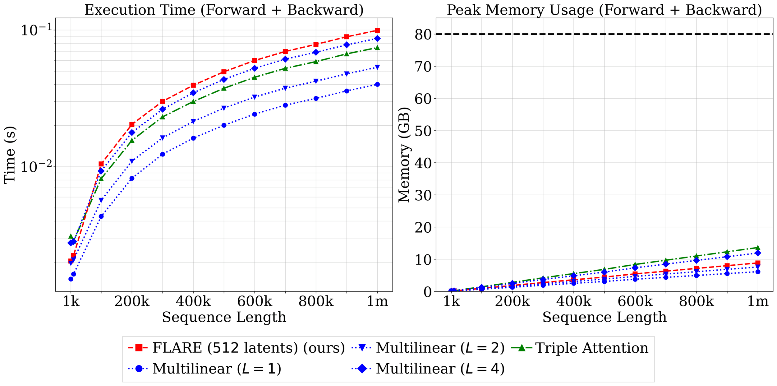
Largest experiment on a single GPU!
17
[1]
[1] Ashton et al. — “DrivAerML: High-Fidelity CFD Dataset for Road-Car Aerodynamics” (arXiv:2408.11969, 2024)
18
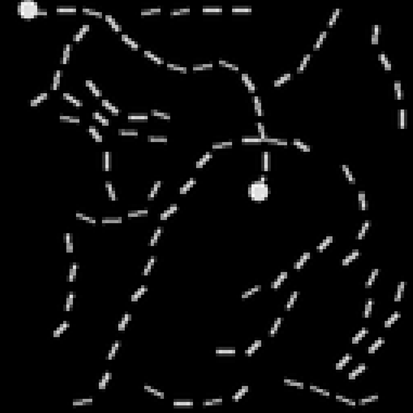
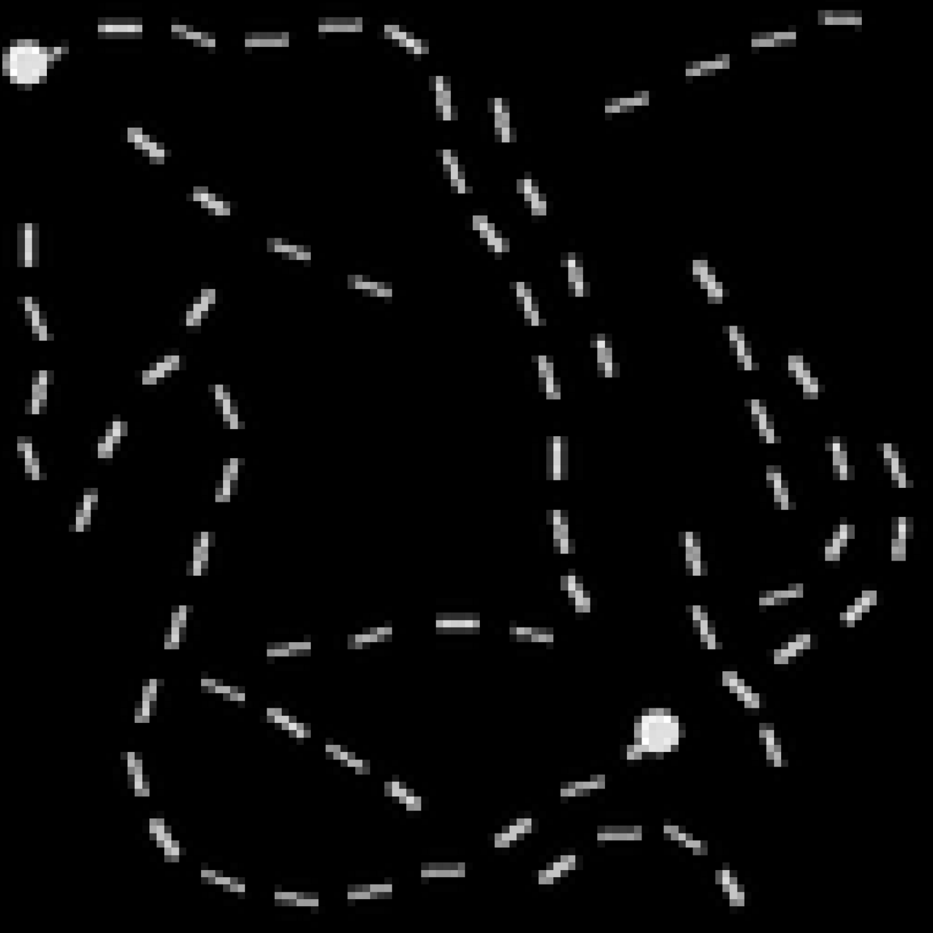
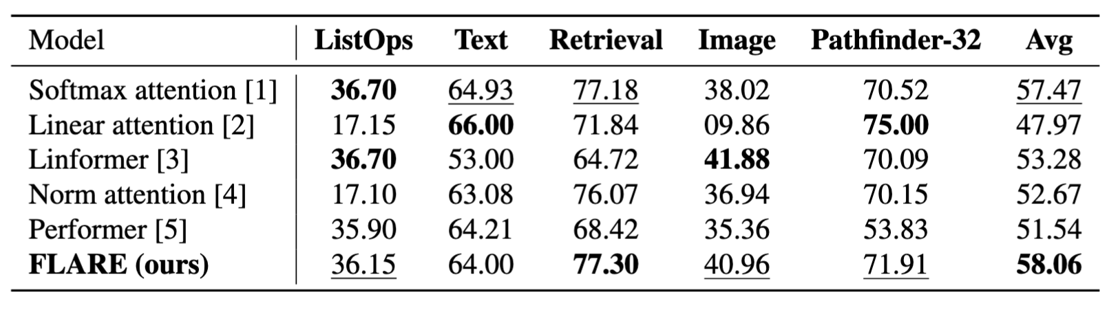
Pathfinder
Listops
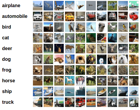
Image classification
Text sentiment analysis
[7]
[8]
[1]
[5]Choromanski et al. — "Rethinking Attention with Performers", ICLR 2021
[6] Tay, Y. et al. — “Long Range Arena: A Benchmark for Efficient Transformers” (arXiv 2020)
[7] Centric Consulting — “Sentiment Analysis: Way Beyond Polarity” (blog)
[8] Krizhevsky — CIFAR dataset homepage
[6]
Accuracy \((\%)\) (higher is better)
[1] Vaswani et al. — “Attention Is All You Need”, NeurIPS 2017
[2] Katharopoulos et al. — "Transformers are RNNs: Fast Autoregressive Transformers with Linear Attention", ICML 2020
[3] Wang et al. — "Linformer: Self-attention with linear complexity", arXiv:2006.04768 2020
[4] Qin et al. — "The devil in linear transformer", arXiv:2210.10340 2022
19
SOTA model for large scale encoder attention.
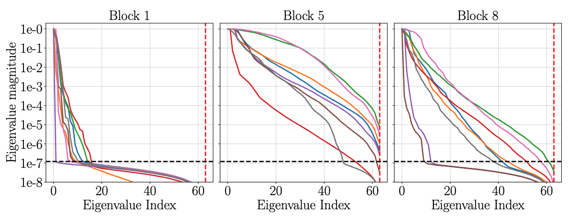
Comprehensive ablations, spectral analysis.
Now implemented in NVIDIA PhysicsNeMo
Ongoing work: decoder attention for transient problems.
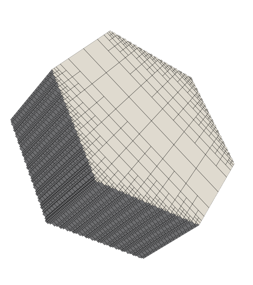
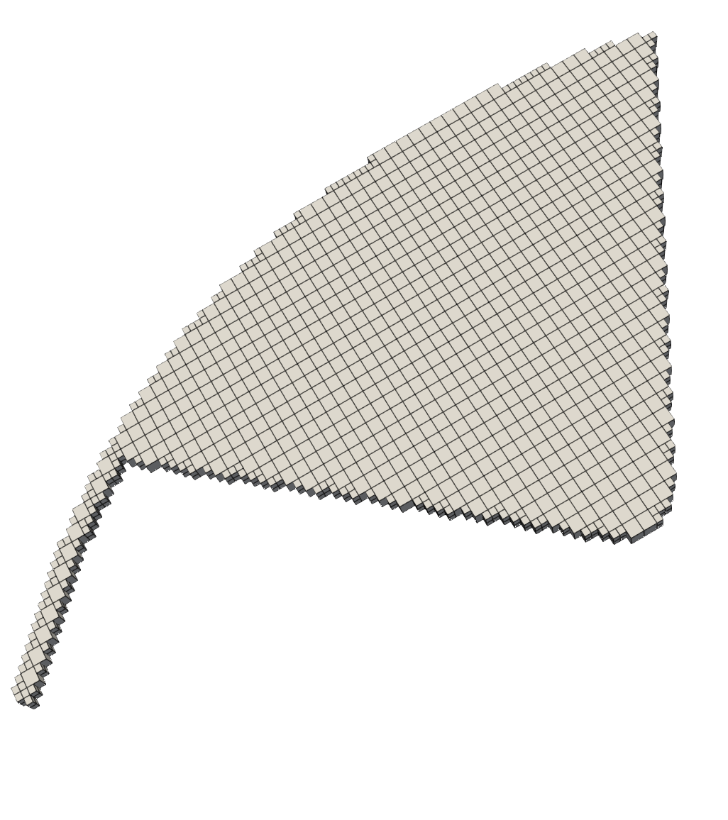
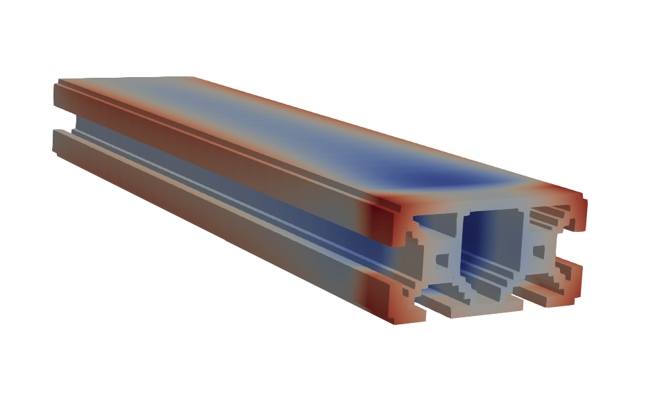
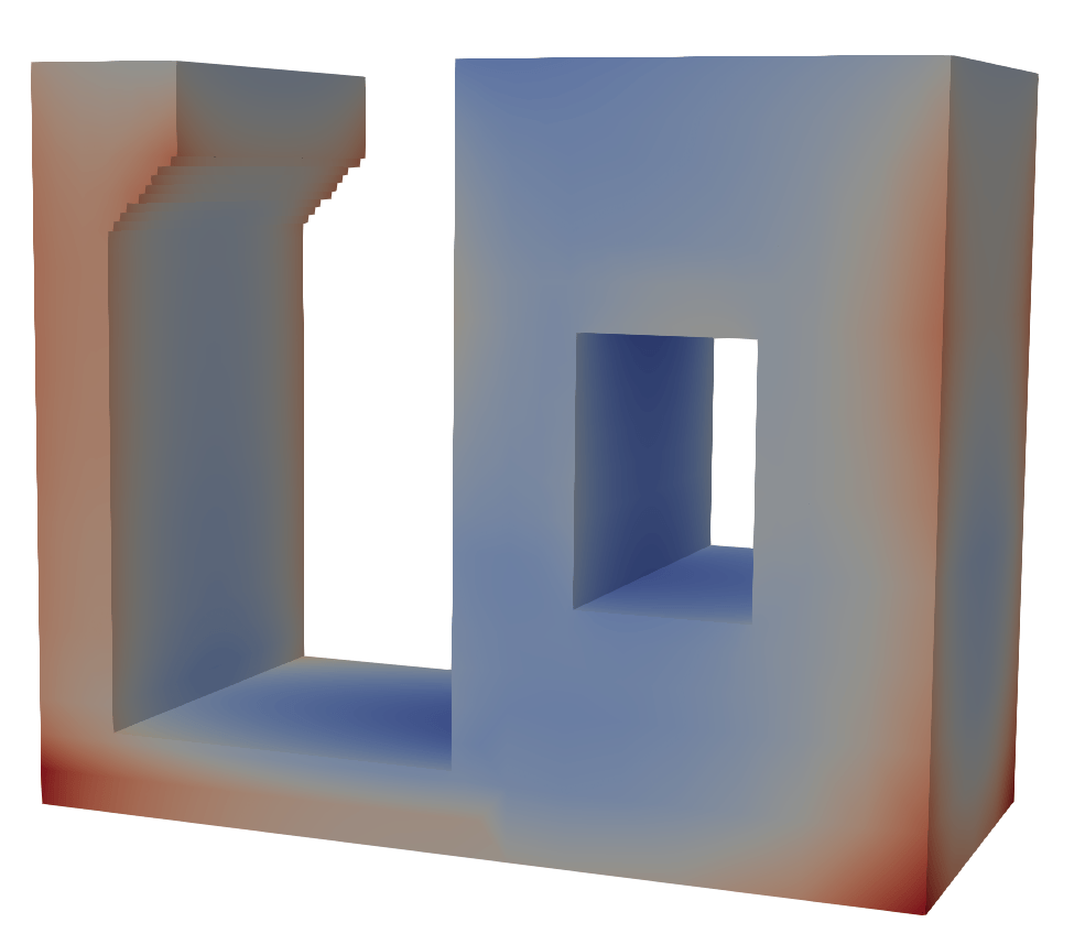
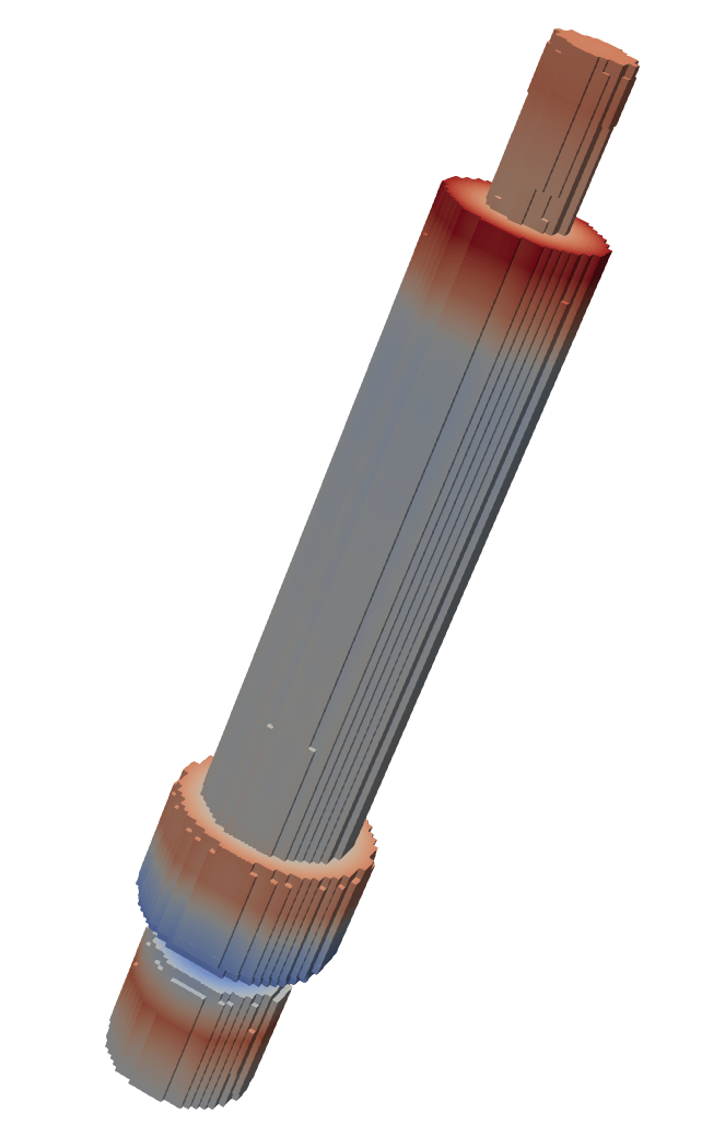
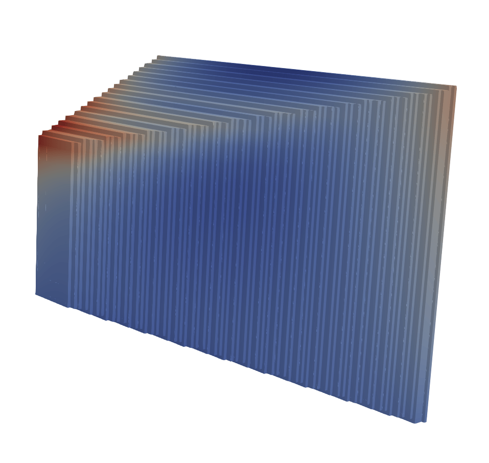
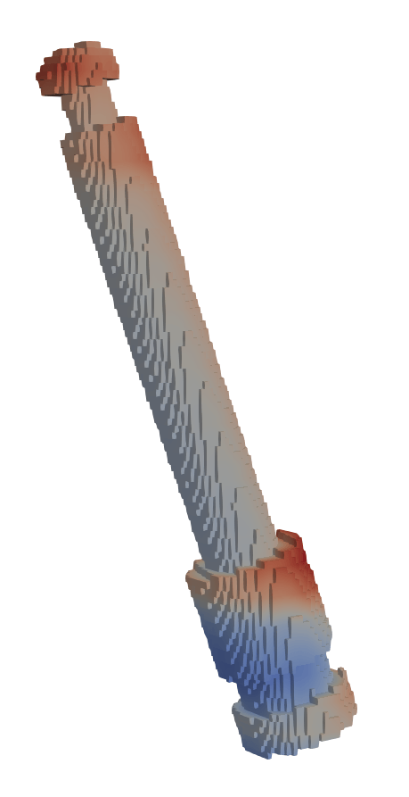
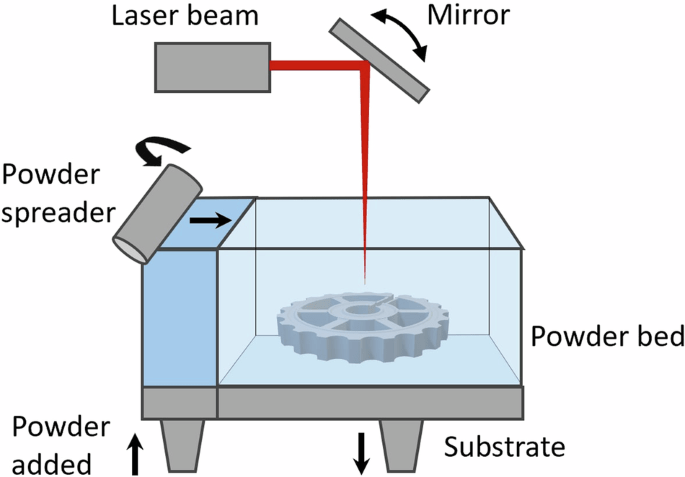
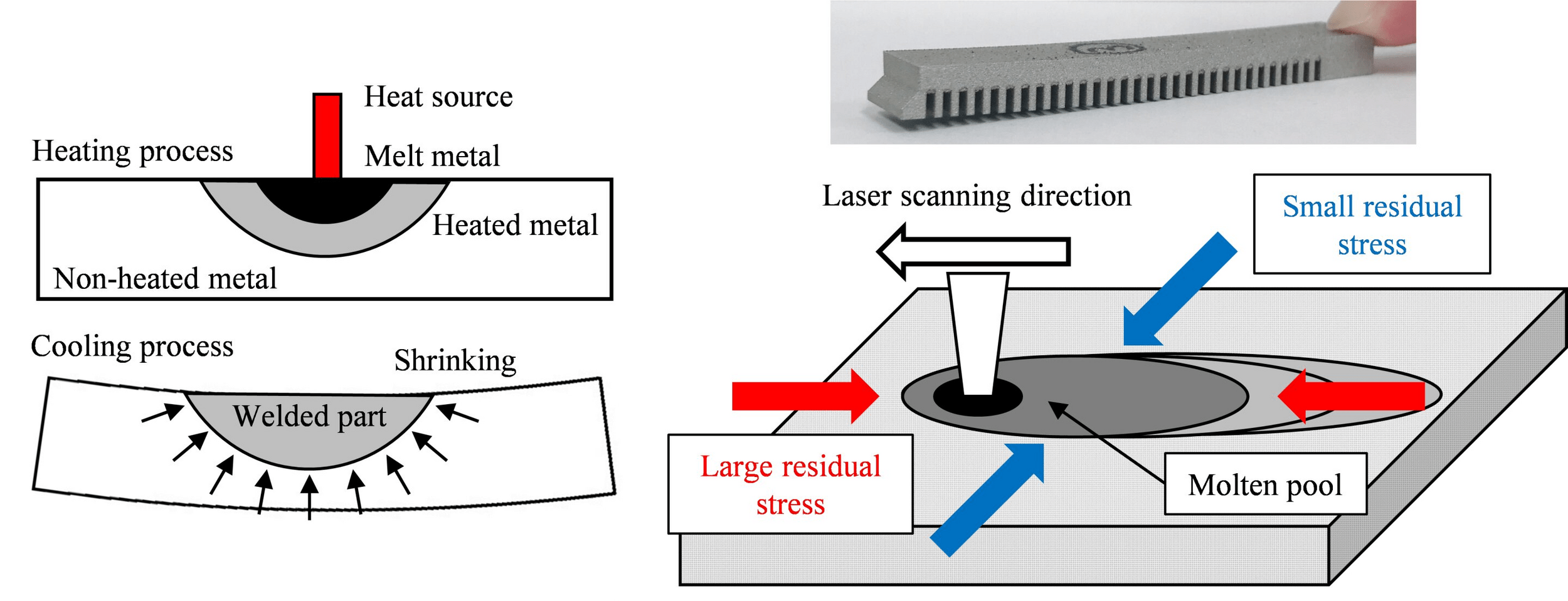
Laser Powder Bed Fusion (LPBF)
Dataset of 20k LPBF calculations
Goal: develop fast surrogate model to predict warpage during build
Governing equations
End results could be deployed as a valuable design tool for metal AM.
20
[1]
[2]
[1] Nature Scientific Data — High-resolution dataset (2025)
[2] TechXplore — “Synergetic optimization reduces residual warpage in LPBF” (2022)
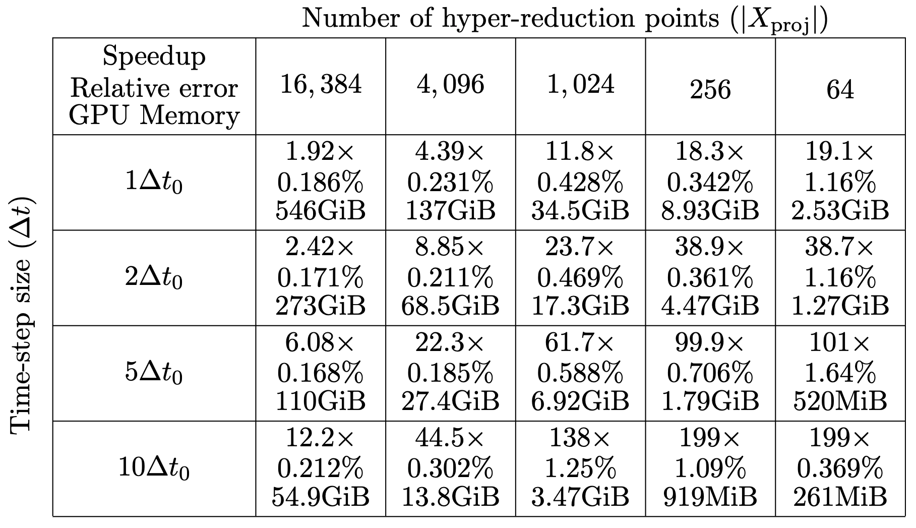
21
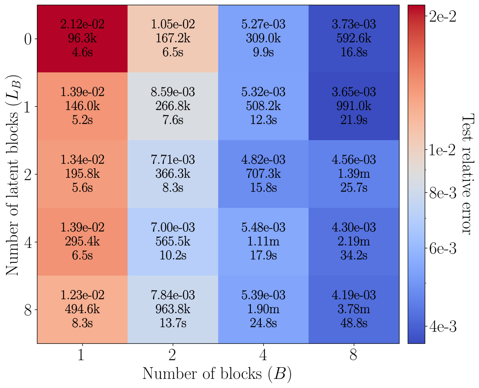
22
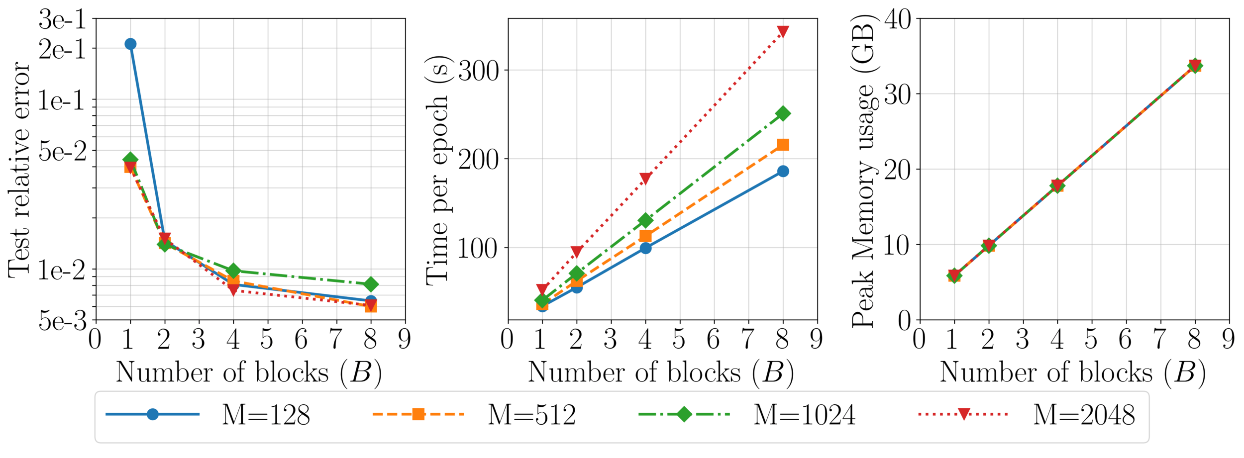
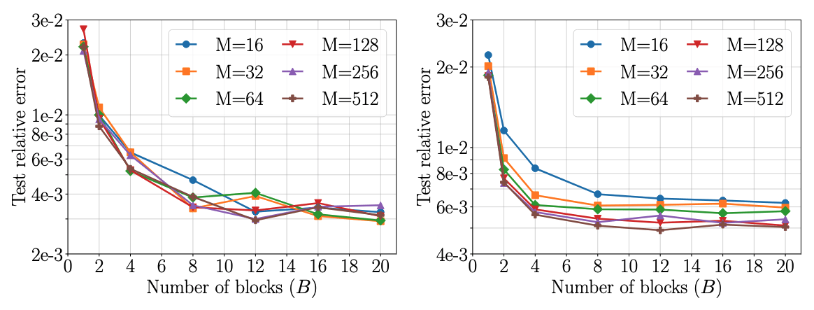
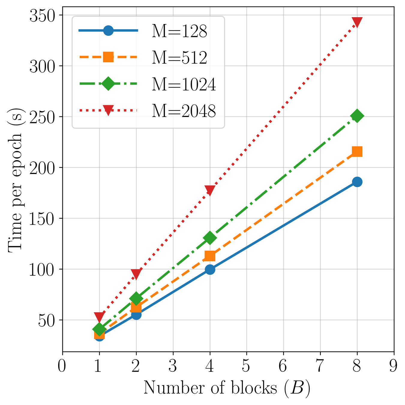
Complexity scales with latents (\(M\)): \(\mathcal{O}(2MN)\)
Accuracy increases with \(M\)
Method: progressively increase latents (\(M\)) through training.
Challenge: Minimize loss spikes, training instabilities.
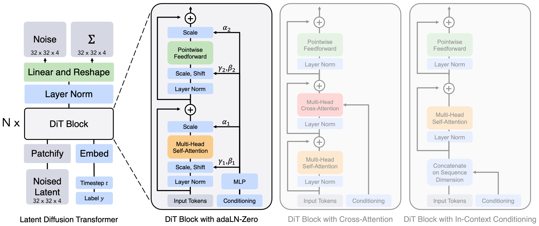
Token mixing [1] (\(\mathcal{O}(N^2)\))
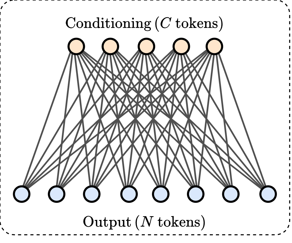
Conditioning [1] (\(\mathcal{O}(N\cdot C)\))
Token mixing
Token mixing
Conditioning
23
[1] Vaswani et al. — “Attention Is All You Need”, NeurIPS 2017
Key idea: Modulate token-mixing with conditioning tokens
Cross FLARE
24
\(\mathcal{O}(2MN + MC) \) complexity
All previous key/value \(\{k_\tau, v_\tau \}_{\tau \leq t}\) must be cached on the GPU.
Major memory and latency bottleneck!
25
[1] Vaswani et al. — “Attention Is All You Need”, NeurIPS 2017
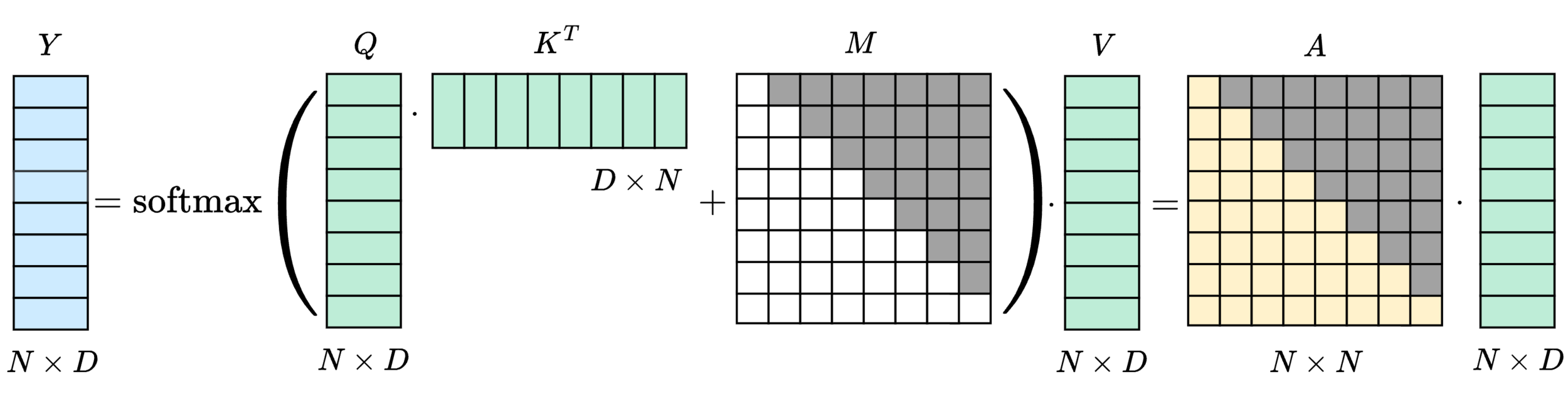
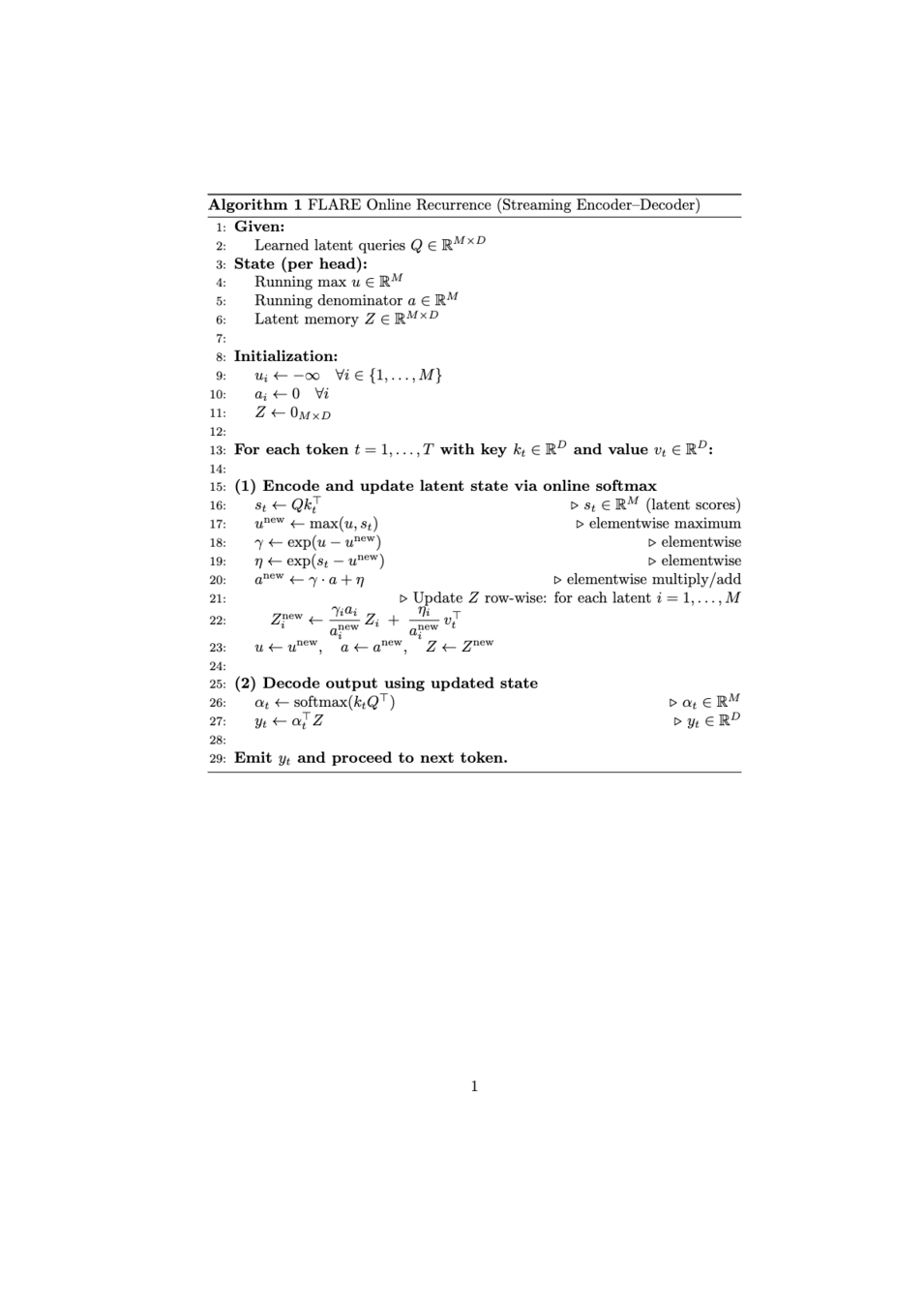
Training algorithm (causal masking)
Inference algorithm (recurrence relation)
Dot-products need to be recomputed for every \(q_t\).
\(\mathcal{O}(N^2)\) complexity.
Linear time auto-regressive attention.
Fixed memory footprint (only store \(\mathcal{O}(M)\) cache).
Flexible latent capacity.
Advantages
Required components
Fused GPU kernels for training and inference.
Bespoke training algorithm for causal FLARE.
Extensive benchmarking and evaluation.
26
Inference algorithm (recurrence rule)
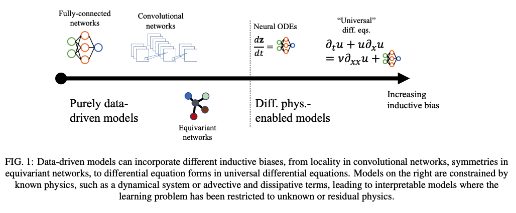
Landscape of ML for PDEs
Mesh ansatz
PDE-Based
Neural Ansatz
Data-driven
FEM, FVM, IGA, Spectral
Fourier Neural Operator
Neural Field
DeepONet
Physics Informed NNs
Convolution NNs
Graph NNs
Adapted from Núñez, CEMRACS 2023
Neural ODEs
Universal Diff Eq
Reduced Order Modeling
| Orthogonal Functions | Deep Neural Networks |
|---|---|
|
|
|
|
|
|
|
|
\( N \) parameters, \(M\) points
\( h \sim 1 / N \) (for shallow networks)
\( N \) points
\( \dfrac{d}{dx} \tilde{f}\sim \mathcal{O}(N^2) \) (exact)
\( \dfrac{d}{dx} \tilde{f} \sim \mathcal{O}(N) \) (exact, AD)
\( \int_\Omega \tilde{f} dx \sim \mathcal{O}(N) \) (exact)
(Weinan, 2020)
\( \int_\Omega \tilde{f} dx \sim \mathcal{O}(M) \) (approx)
Model size scales with signal complexity
Model size scales exponentially with dimension
\( N \sim h^{-d/c} \)
FEATURES
DEMONSTRATIONS
Challenge: Learn PDE surrogate on 5-10 m points on multiGPU cluster
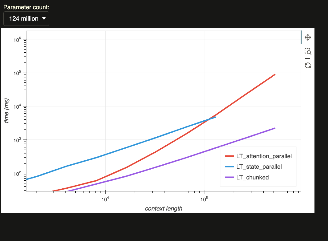
Linear transformers replace the softmax kernel with a feature map \(\phi(\cdot)\) such that
This factorization allows causal attention to be computed recurrently:
https://manifestai.com/articles/linear-transformers-are-faster/
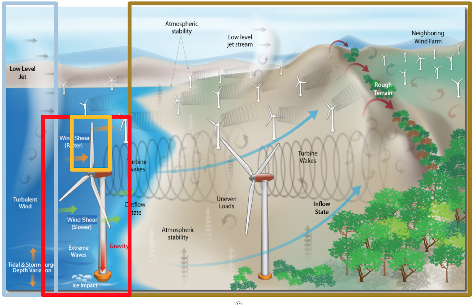
Mesosphere
Wind farm
Turbine
Blade
1
Modern engineering is reliant on computer simulations
Design space exploration
Predictive maintenance
[1]
[2]
24
Message-passing is fundamentally low-rank
25
13
\(\text{CAE-ROM}\) [1]
\(\text{SNFL-ROM (ours)}\)
\(\text{SNFW-ROM (ours)}\)
\(\text{Relative error }\)
[1] Lee & Carlberg — Nonlinear manifold ROM via CNN autoencoders (JCP 2020)
\([1]\)
By Vedant Puri
Vedant Puri's job talk at Meshy.ai


