





Vedant Puri
PhD student at Carnegie Mellon University
Vedant Puri
AUG 19, 2026
L = MSE(u_true - u_pred)
u_pred = NN(x) <-- current situation
u_pred = NN(x) + u_linear_approx
u_linear_approx_{x,y} = 0
u_linear_approx_x = XXX
NN: [N, D] -> [N, Do]
final hidden states h [N, C=128]
u_pred = h * W [C, Do] --> [N, Do]
u_sca_pred = pool(h) * W [C, 1]
L = MSE(u_pred, u_true) + lambda * MSE(u_pred_sca, u_sca)
pool: [N, C] -> [1, C] # mean pooling, class-pooling
1
Predictive maintenance
Design space exploration
[2]
[1]
[3]
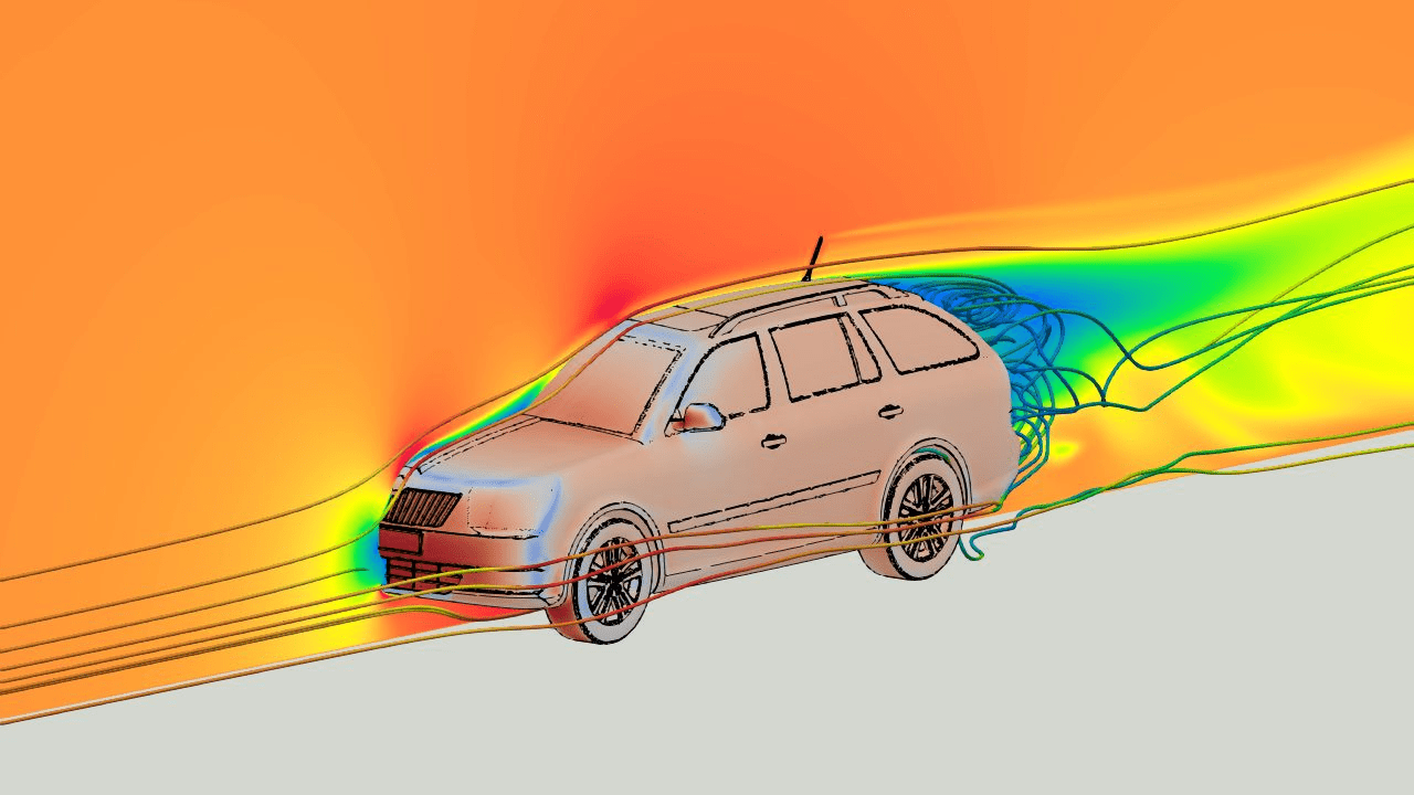
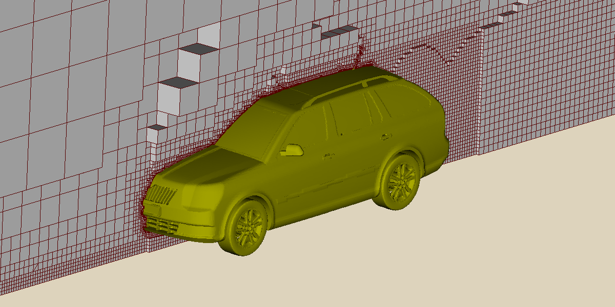
[1] CFD Direct / OpenFOAM – “OpenFOAM HPC on AWS with EFA”, cfd.direct
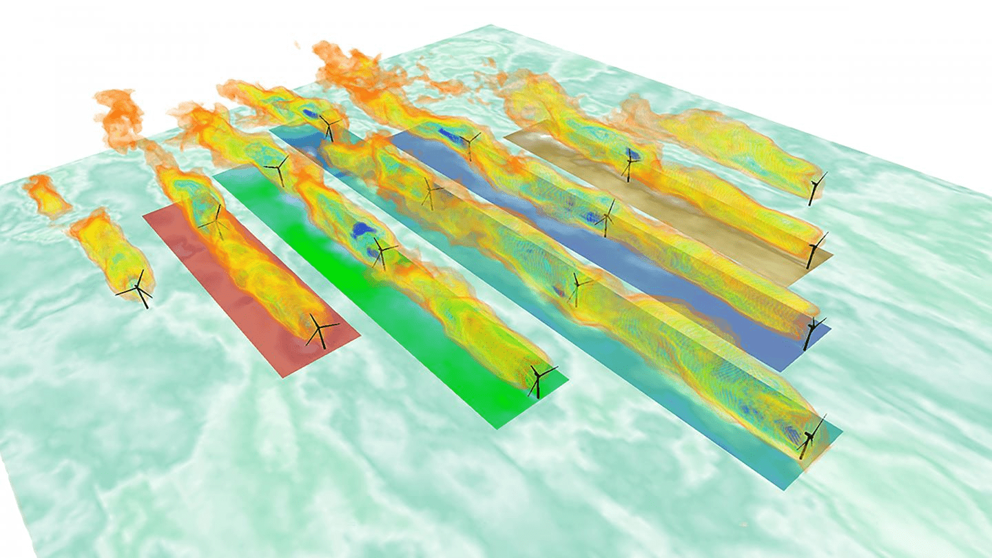
[2] EurekAlert — “New concrete system may reduce wind-turbine costs”
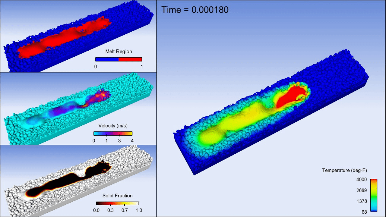
[3] Flow-3D, “FLOW-3D AM” product page, flow3d.com
Process optimization
[1]
2
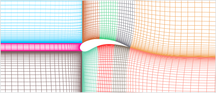
[1] GridPro Blog — “The Art and Science of Meshing Airfoil”
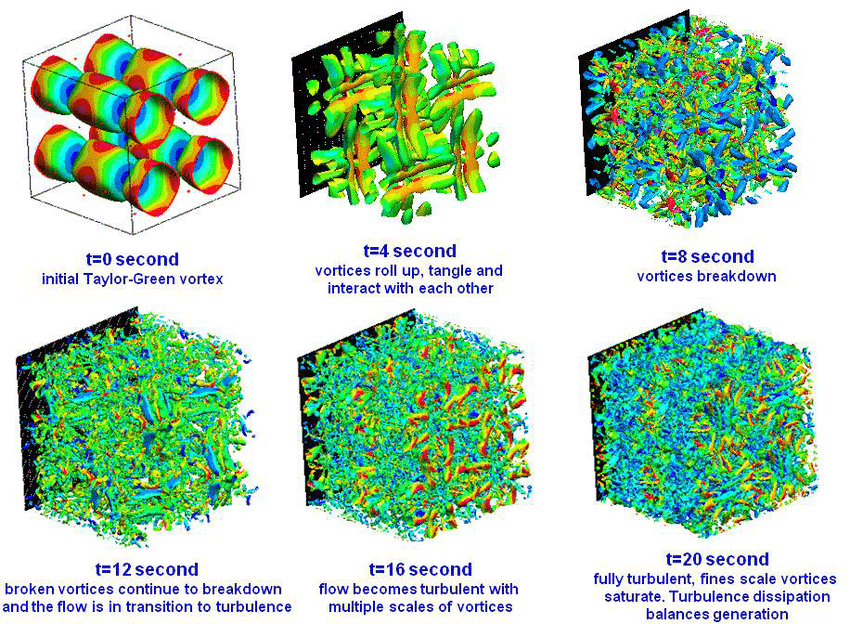
[2] ResearchGate — “Transition to turbulence of Taylor-Green Vortex at different time (DNS)” (figure)
[3] ORNL / U.S. Department of Energy — “DOE and Cray deliver record-setting Frontier supercomputer at ORNL”
[1]
Complex geometry \(\implies\) many DoFs
Multiscale physics \(\implies\) small \(\Delta t\)
[2]
Repeated large system solves
[3]
3
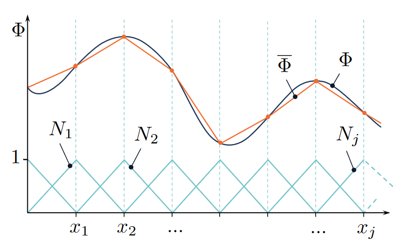
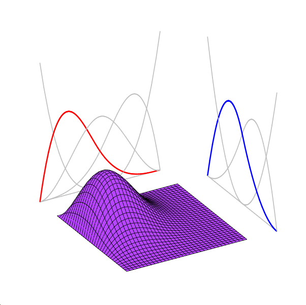
(Explicit) Weighted sum of polynomial interpolants
[1]
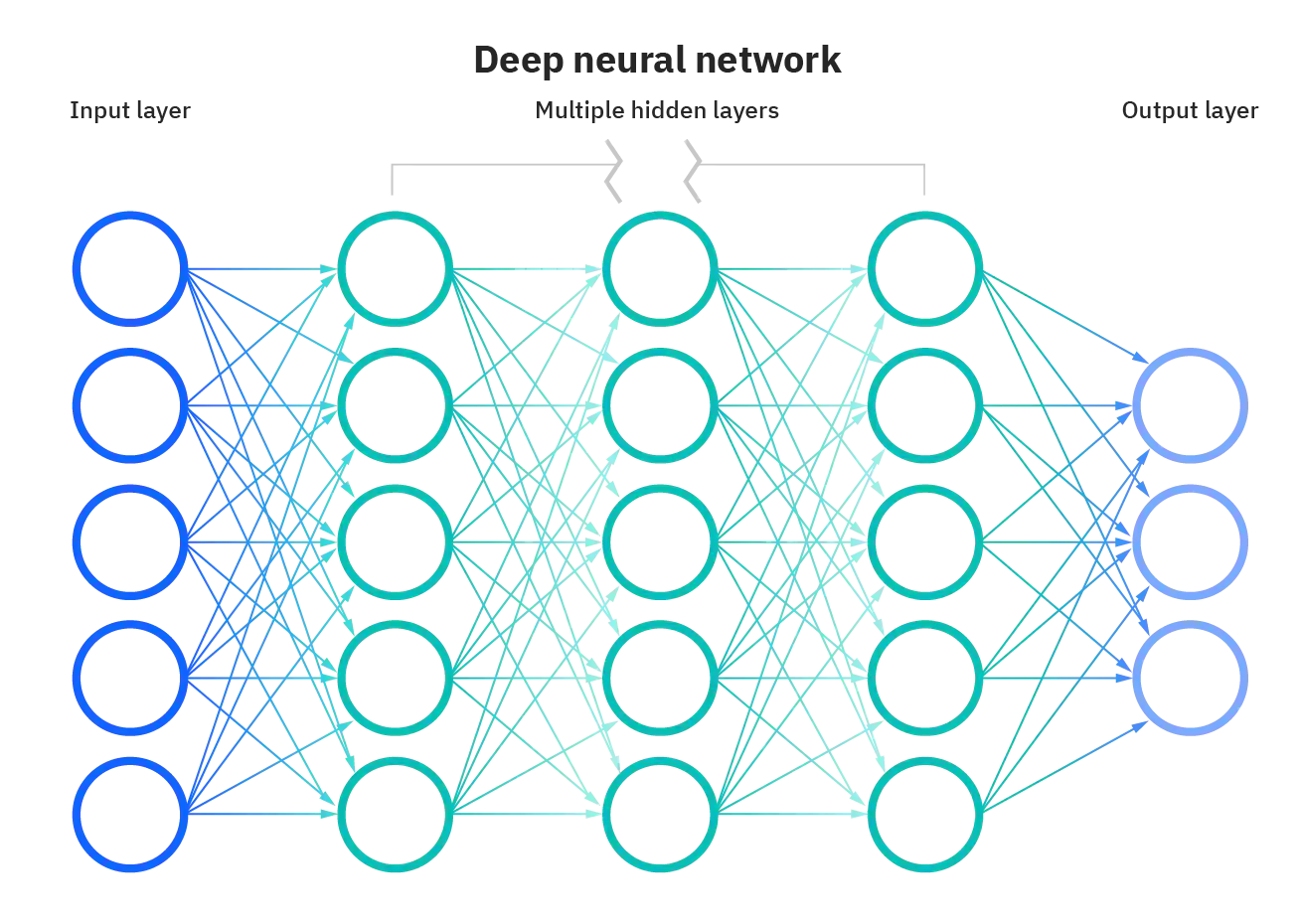
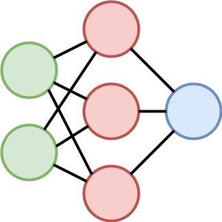
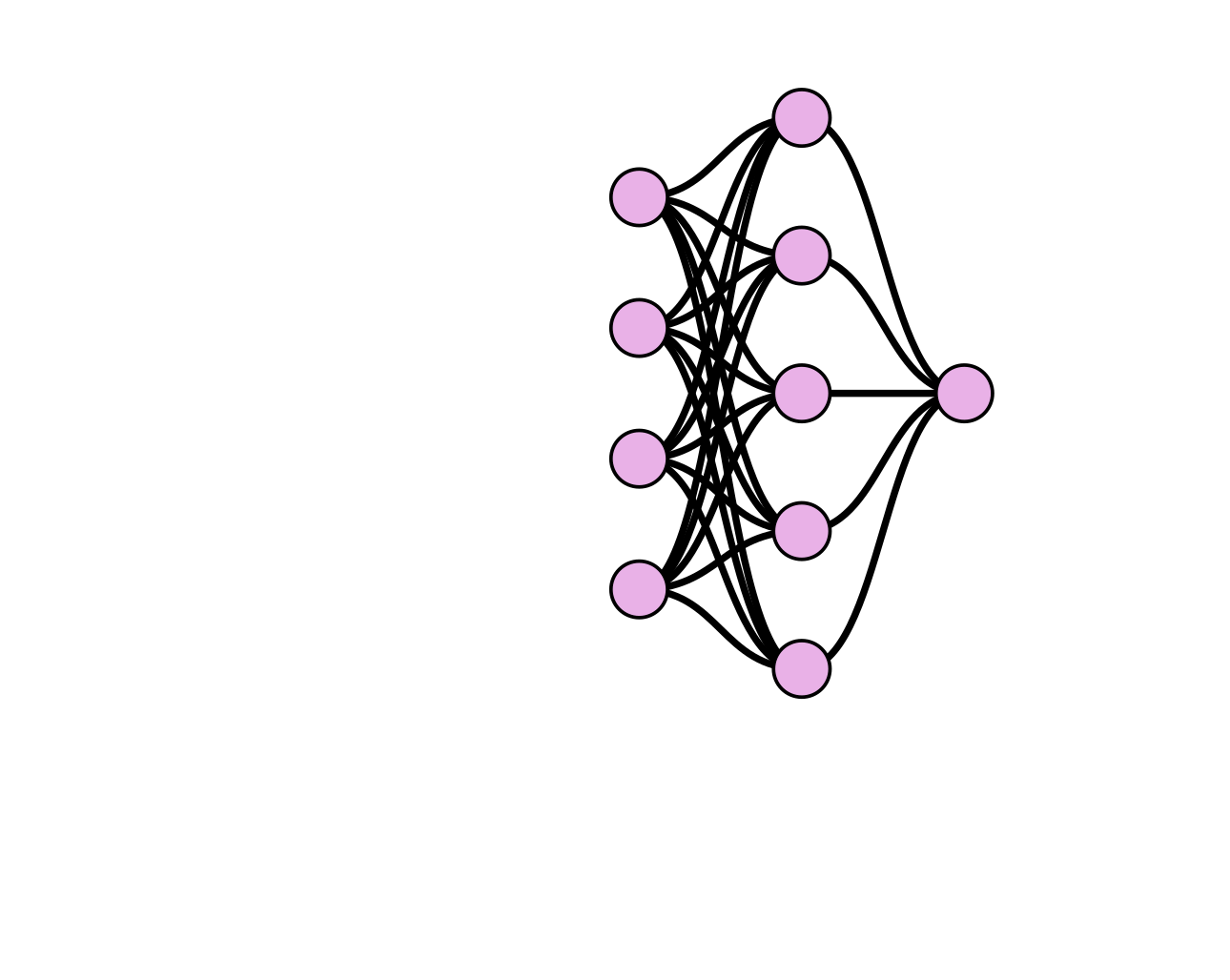
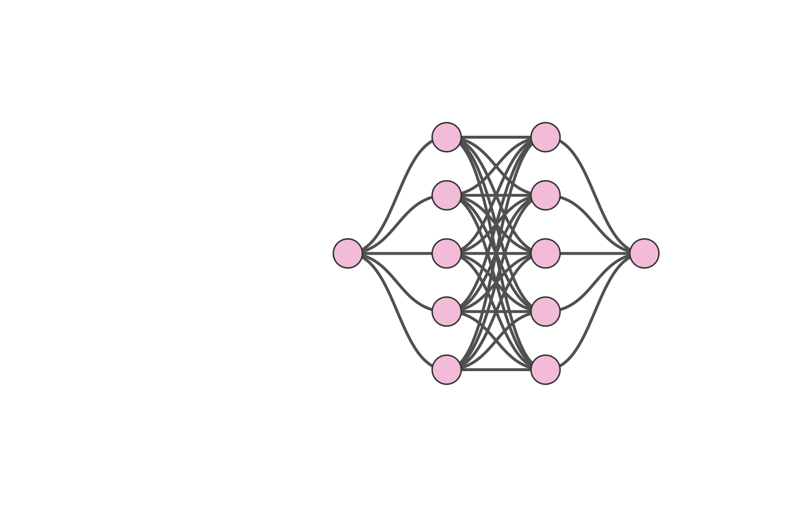
(Implicit) High-dim nonlinear feature learners
[2]
Cannot learn from data
Can learn from data
Large cost per simulation
Cheap evaluation after training
High-accuracy
Problem-specific
Robust
Up to \(0.1\%\) accuracy
[1] Math StackExchange — “Interpolation in Finite Element Method”
[2] ResearchGate — “Structure of a Deep Neural Network” (figure)
\(\text{Mesh ansatz}\)
\({u}(x)=\)
\(u(x) = \)
\(\text{Neural ansatz}\)
\(\text{Physics-based}\)
\(\text{Data-driven}\)
\(\text{Numerical simulation}\)
\(\text{Reduced Order Modeling}\)
\(\text{Neural ROMs}\)
\(\text{Surrogate learning}\)
\(\text{Transformers}\)
\(\text{PINNs}\)
\(\text{Finite Elements}\)
\(\text{PCA/POD}\)
\(\text{Graph Networks}\)
Accelerate numerical solvers with neural ROMs
4
Efficient attention models for large-scale surrogate learning
[1]
[3]
[2]
[1] CFD Direct / OpenFOAM, “Introduction to Computational Fluid Dynamics”
[3] Kutz, J. N. “Data-Driven Modeling & Dynamical Systems” (UW)
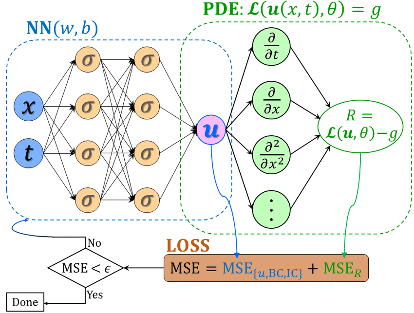
[2] ResearchGate, “Schematic of a Vanilla Physics-Informed Neural Network”
5
Accelerate PDE solves with structure learned from data.
Replace simulation with solution operator learned from data.
Improved accuracy with smarter compression.
6
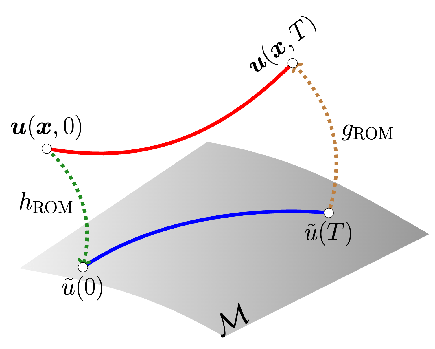
Learn low-dimensional spatial representation with data + evolve with physics.
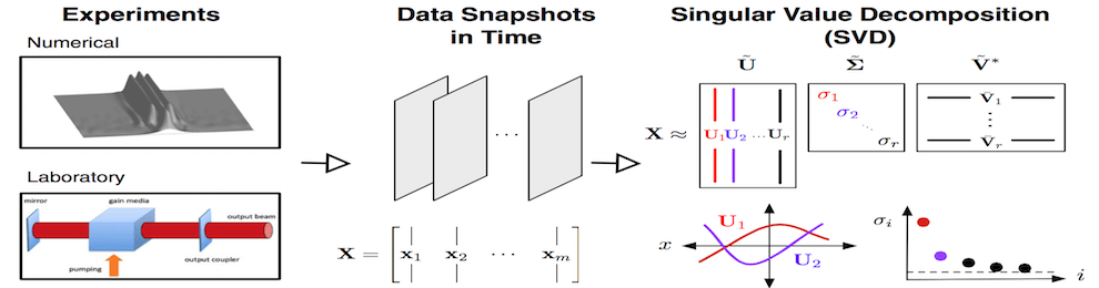
High-dimensional simulation data
Collect and compress data
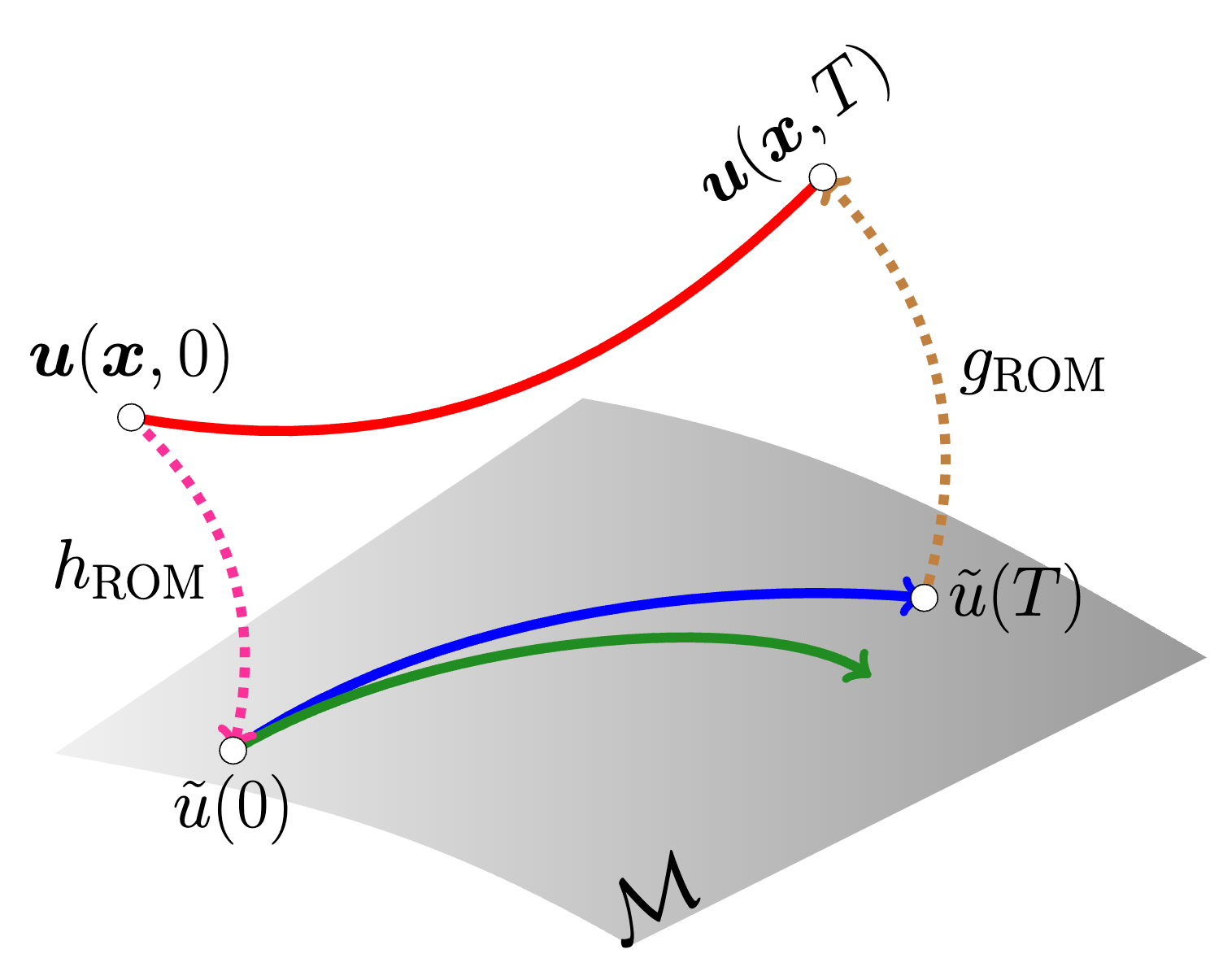
Evolve ODE on low-dim manifold
Cost savings from solving smaller ODE system.
7
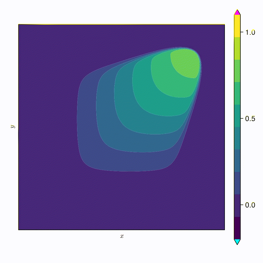
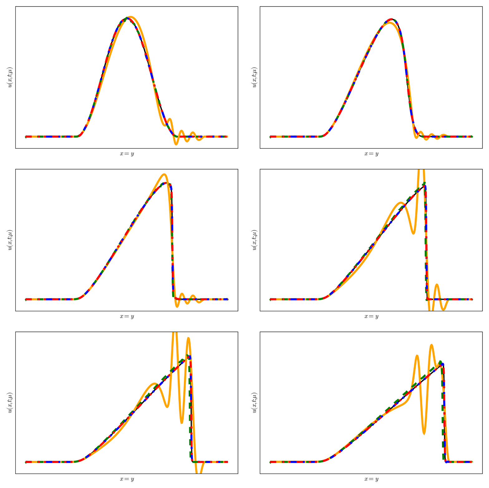
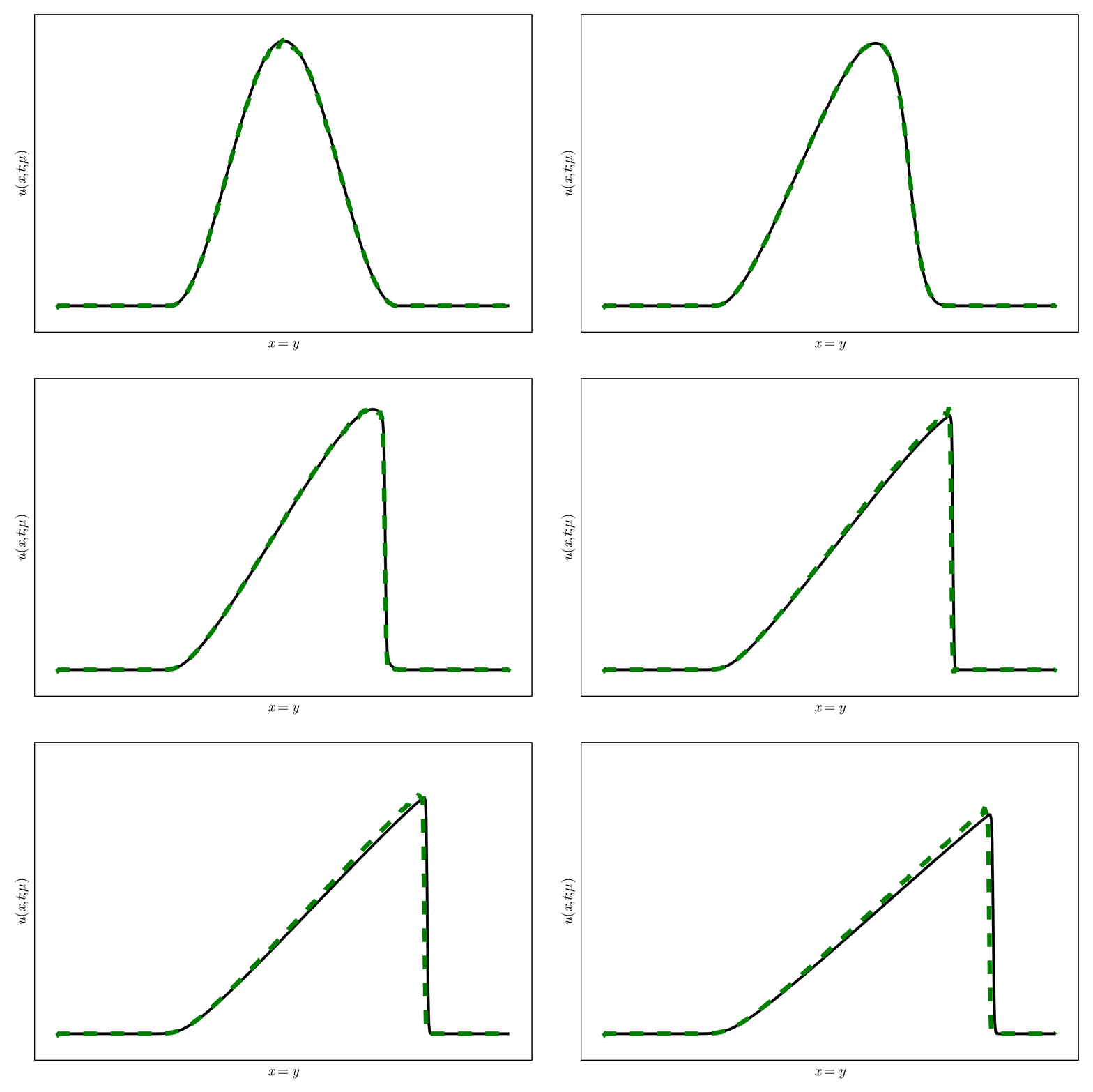
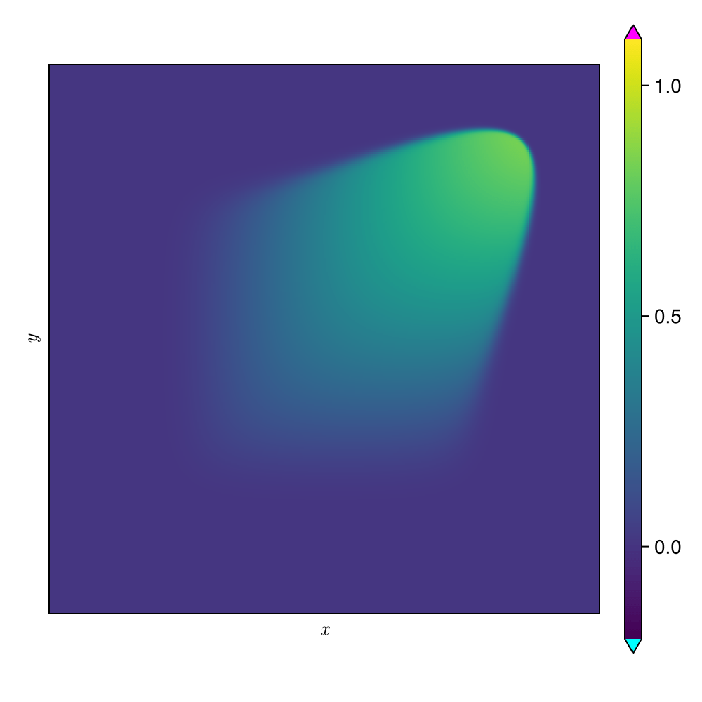
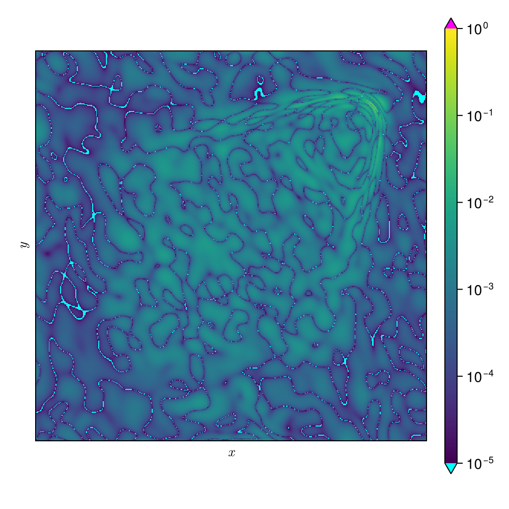
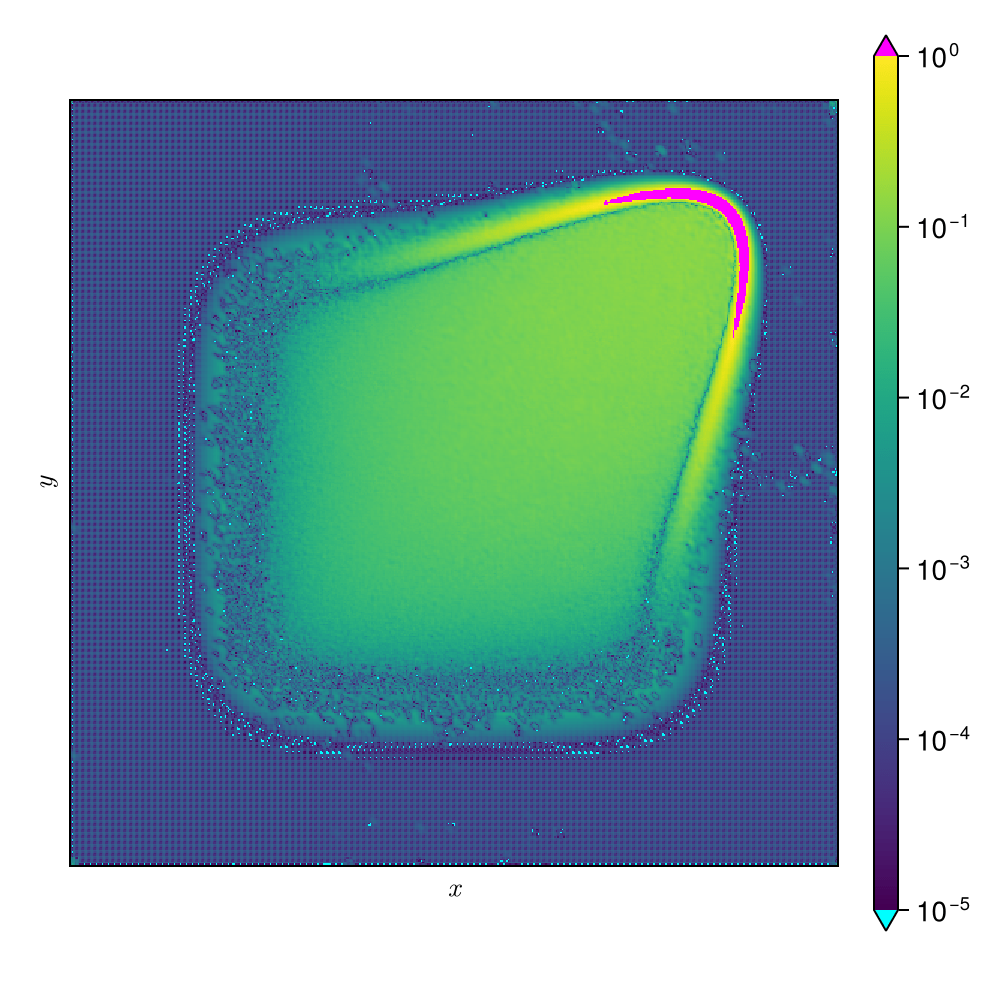
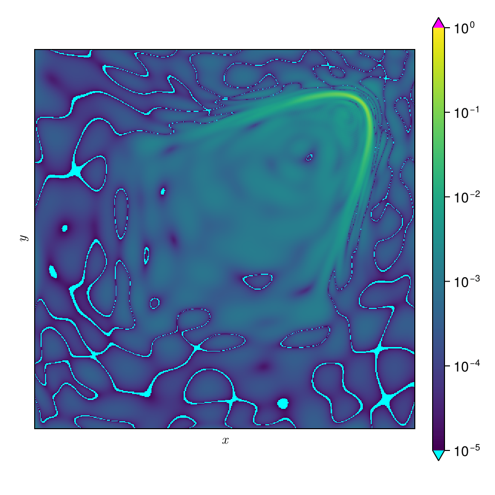
2D Viscous Burgers problem \( (\mathit{Re} = 1\text{k})\)
\(\text{Relative error: }0.37\%\)
\(\text{DoFs: }524~k \to 2\)
\(\text{Wall-time: }13.4~\text{s} \to 0.068~\text{s}\)
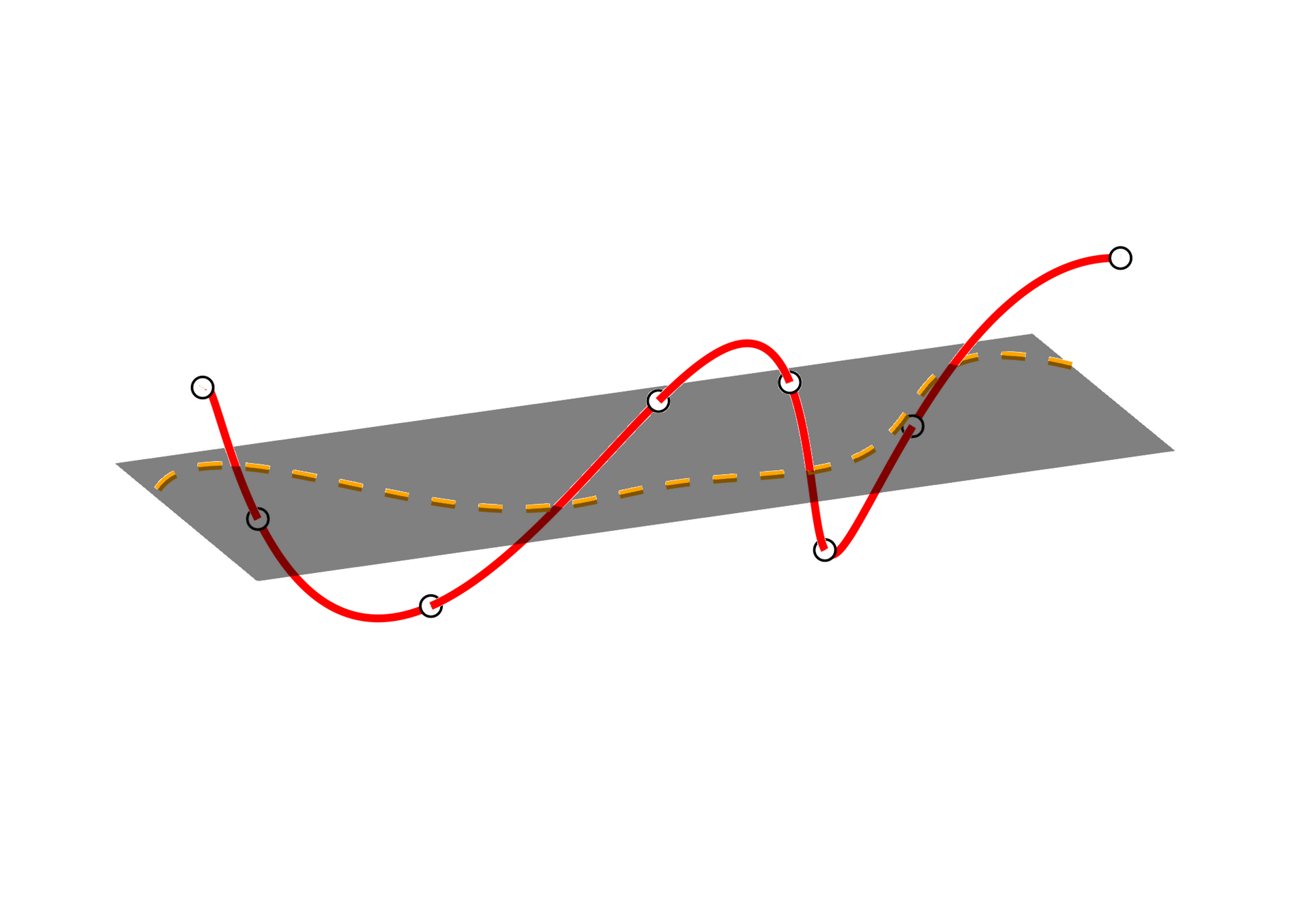
Large deviations!
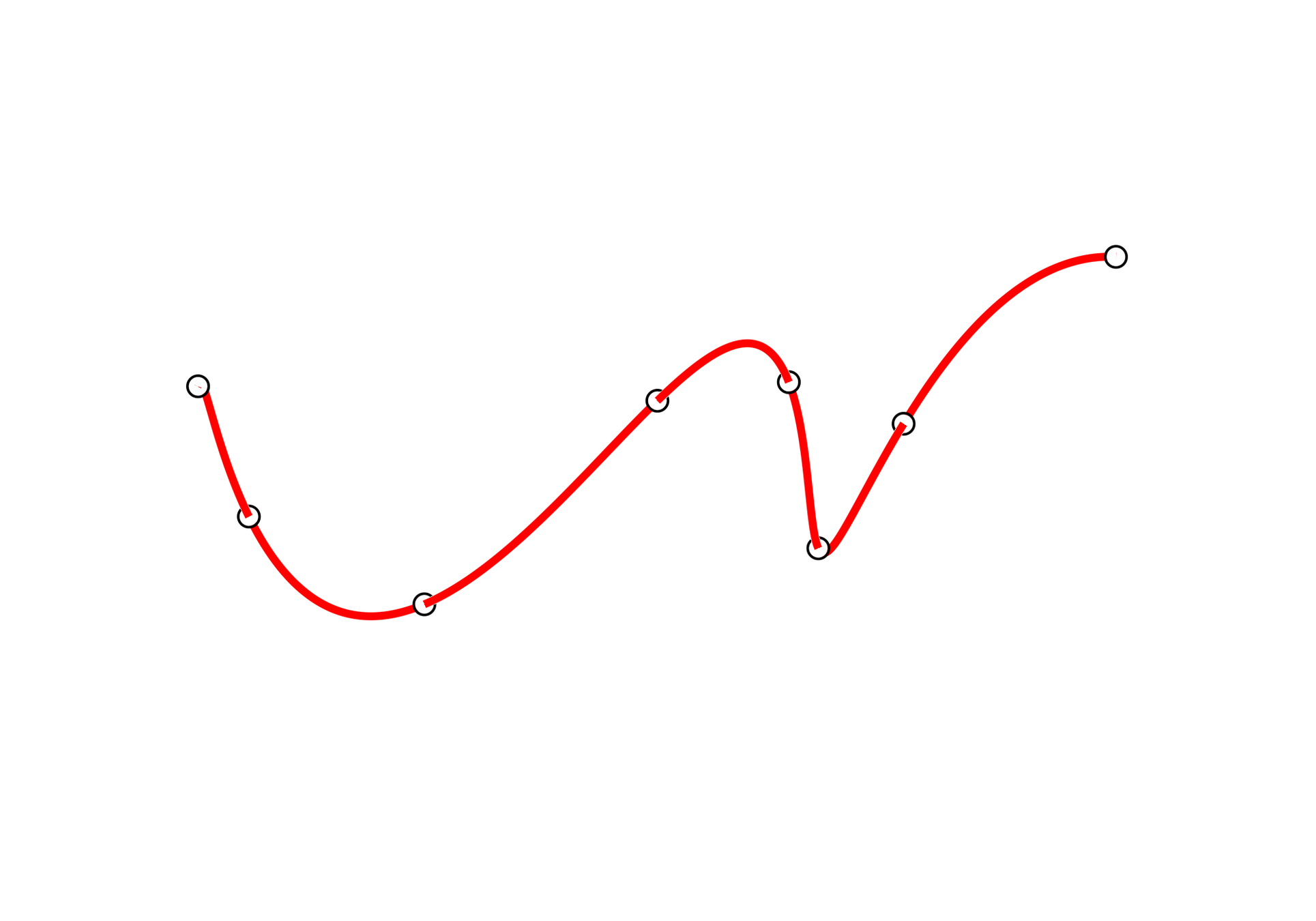
Learning smooth latent space trajectories
\(\text{Autoencoder ROM}\)
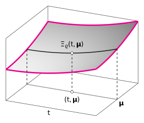
Evolution of ROM states (intrinsic perspective)
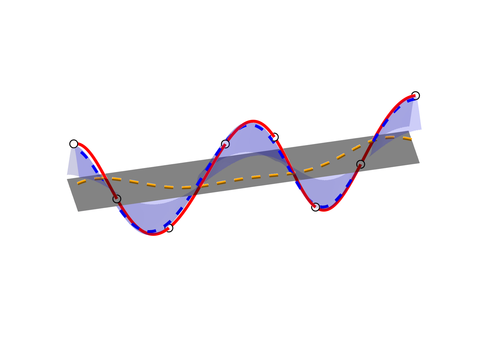
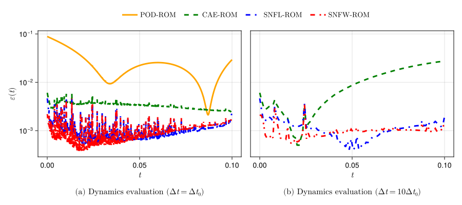
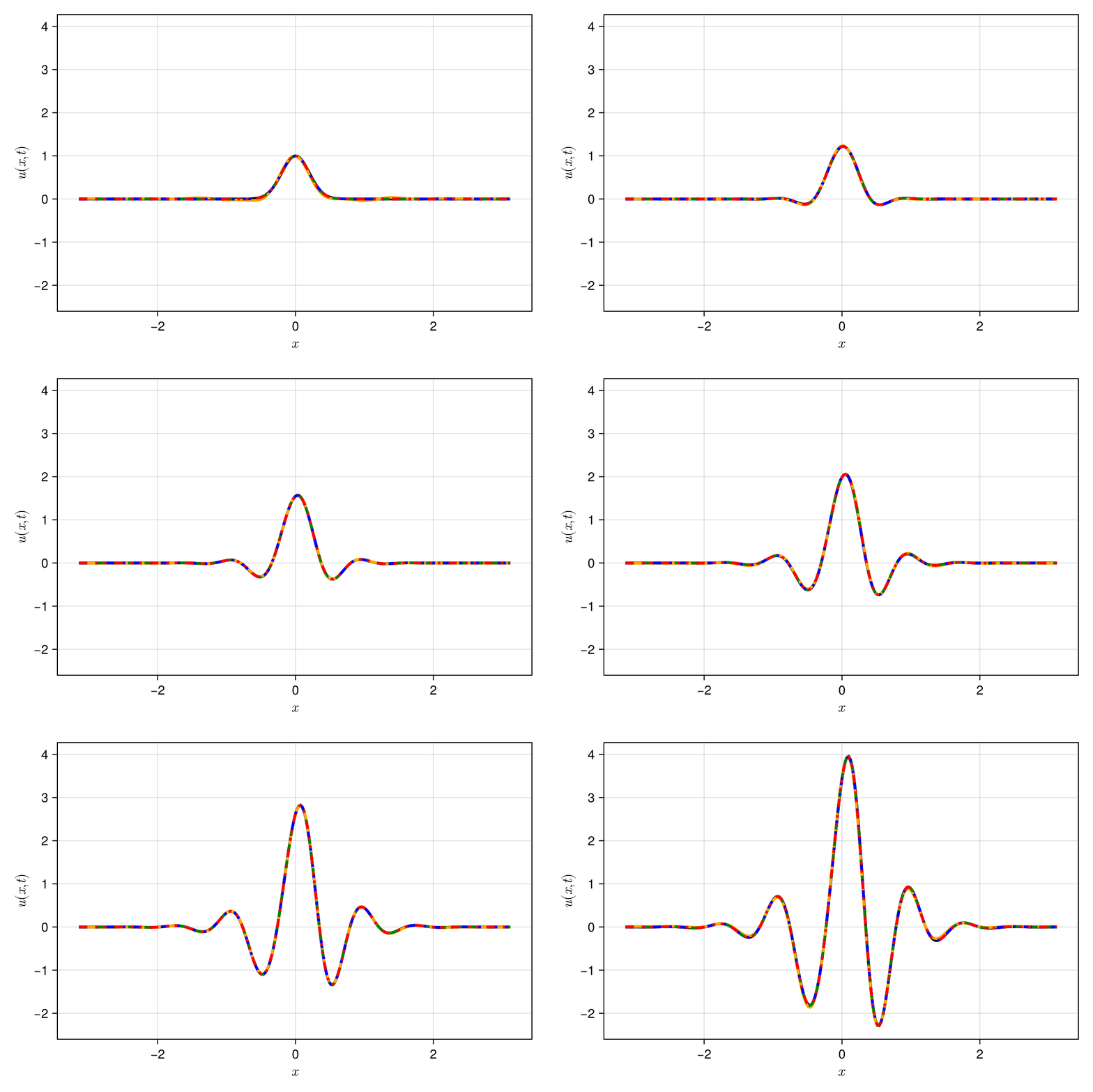
SNF-ROM ensures accurate online dynamics evaluation.
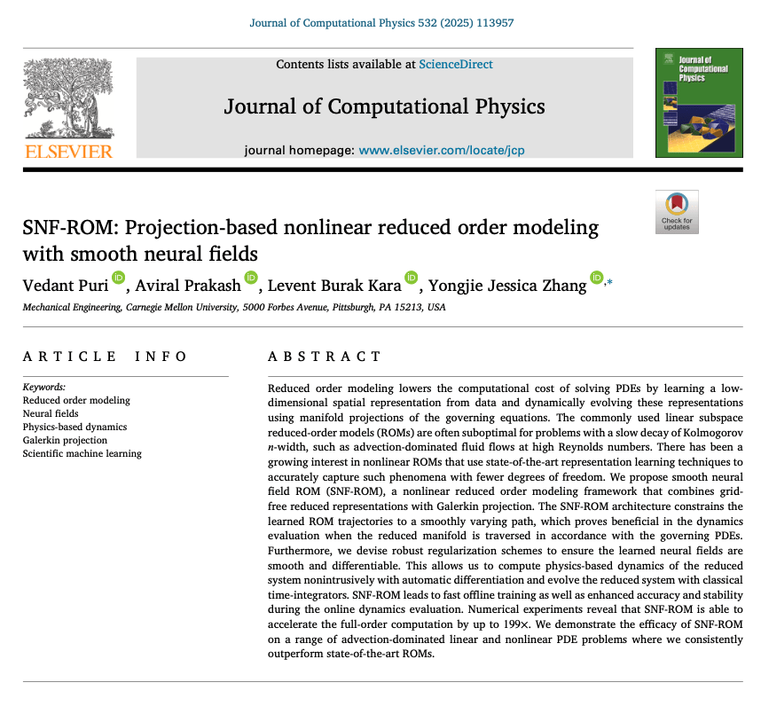
Smooth neural field ROM (SNF-ROM)
7
2D Viscous Burgers problem \( (\mathit{Re} = 1\text{k})\)
\(\text{Relative error: }0.37\%\)
\(\text{DoFs: }524~k \to 2\)
\(\text{Wall-time: }13.4~\text{s} \to 0.068~\text{s}\)
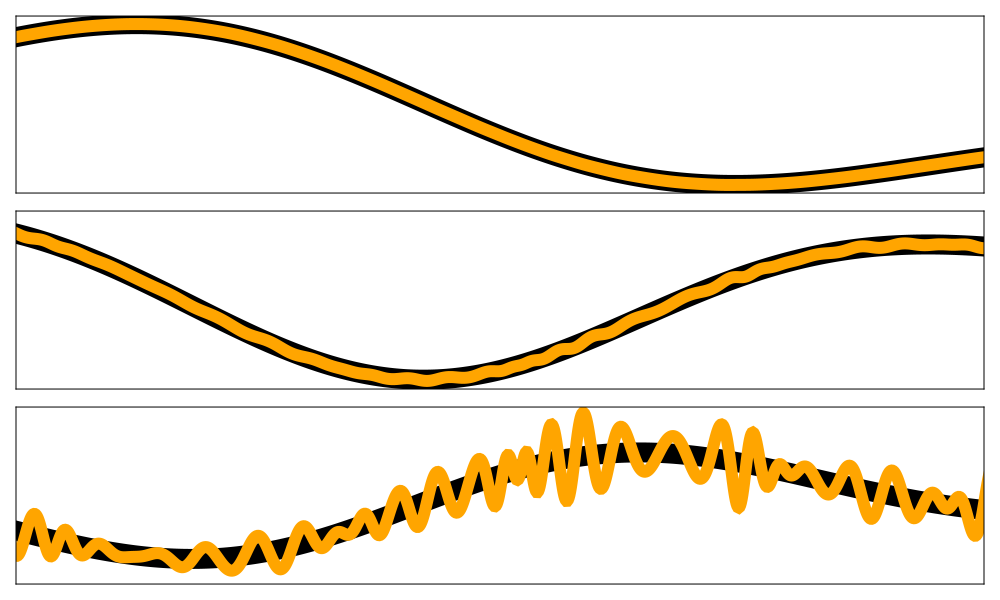
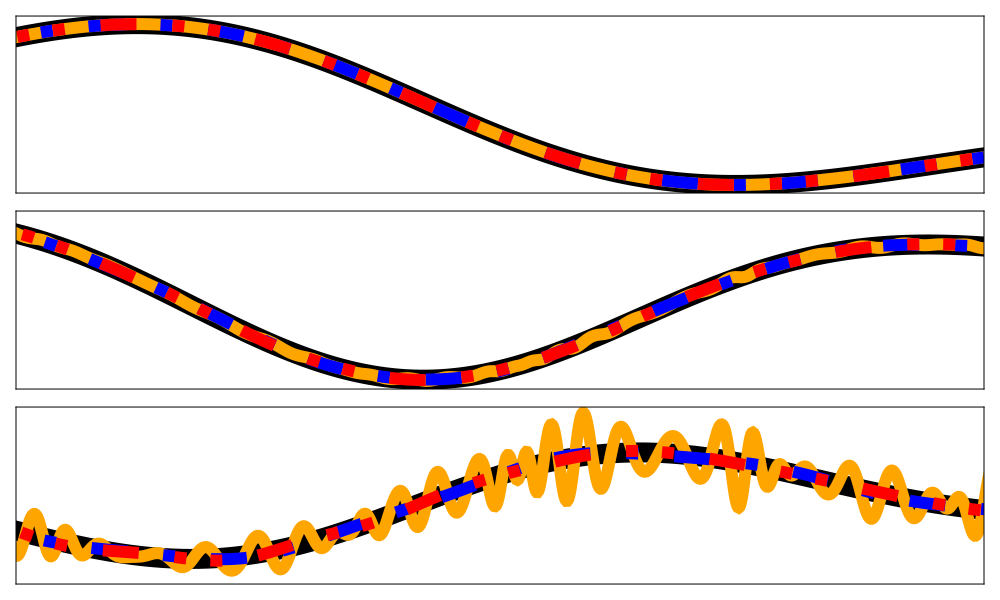
High freq. noise
Non-differentiable!
Accurately capture of dynamics with smooth neural fields
Large deviations!
Learning smooth latent space trajectories
\(\text{Autoencoder ROM}\)
\(\text{SNF-ROM}\)
Evolution of ROM states (intrinsic perspective)
No deviation
SNF-ROM ensures accurate online dynamics evaluation.
Accurate capture of dynamics
Smooth neural field ROM (SNF-ROM)
Won poster award at World Conf. Comp. Mech. 2024
Published in Journal of Comp. Phys.
8
9
Solution operator: dense, global
Forward operator: sparse, local
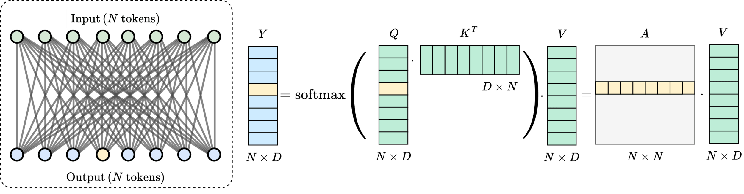
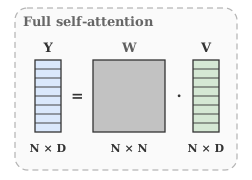
Every point depends on every other
Transformers enable global communication
Message-passing on a dynamic all-to-all graph
[1] Vaswani et al. — “Attention Is All You Need”, NeurIPS 2017
What are the communication requirements of solution operators?
9
[1] Vaswani et al. — “Attention Is All You Need”, NeurIPS 2017
A_{NxN} * u_{Nx1} = f_{Nx1}
u = A ^{-1}_{NxN} * f
u_{Nx1} = NN(f_{Nx1})
(Q(f)_{Nx1} * K(f)_{Nx1}^T)_{NxN} * V(f)_{Nx1}
10
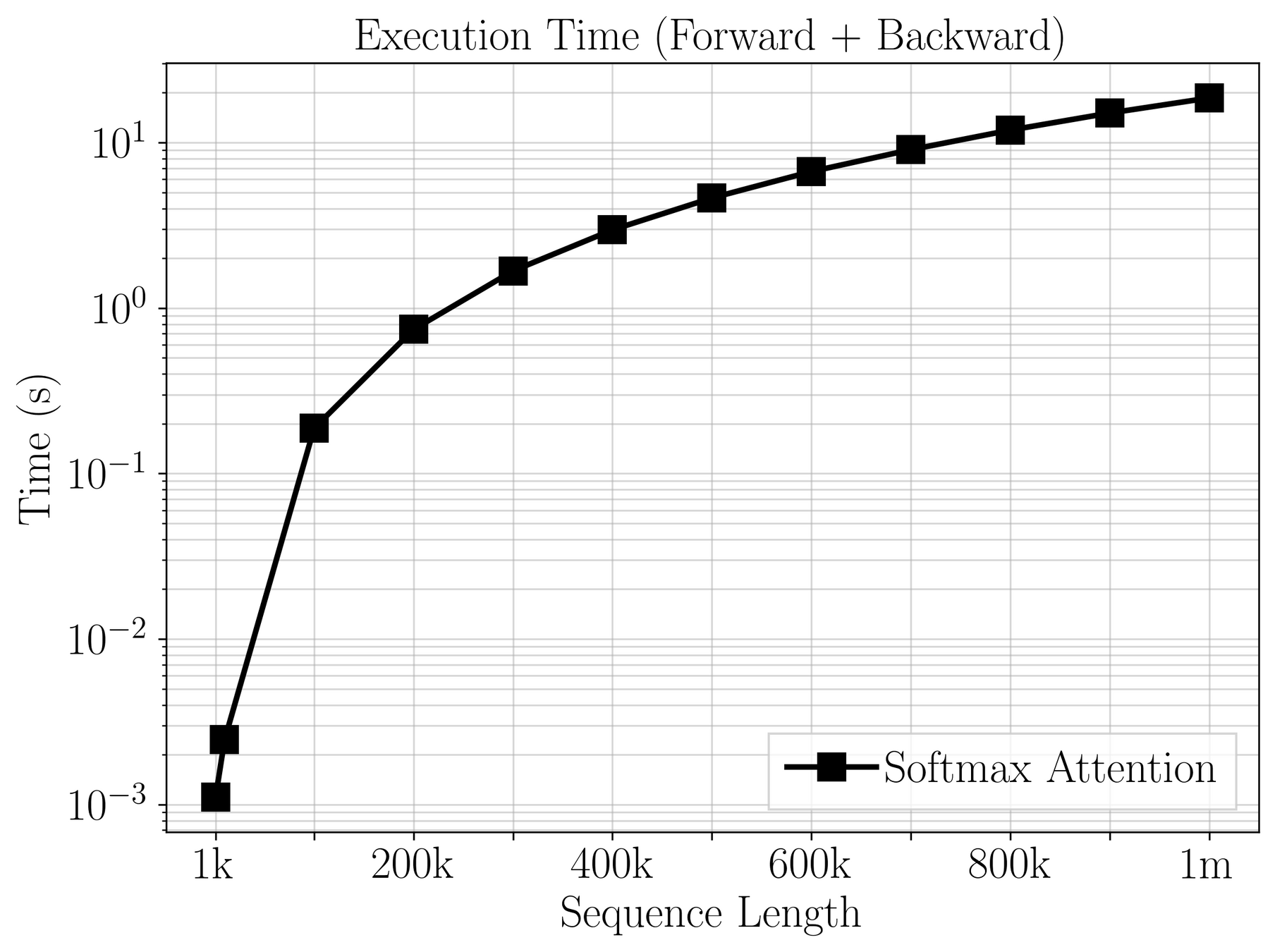
Infeasible for large problems
Over \(20~\text{s}\) per gradient step on 1M points!
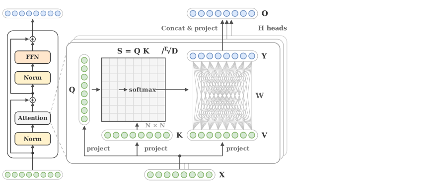
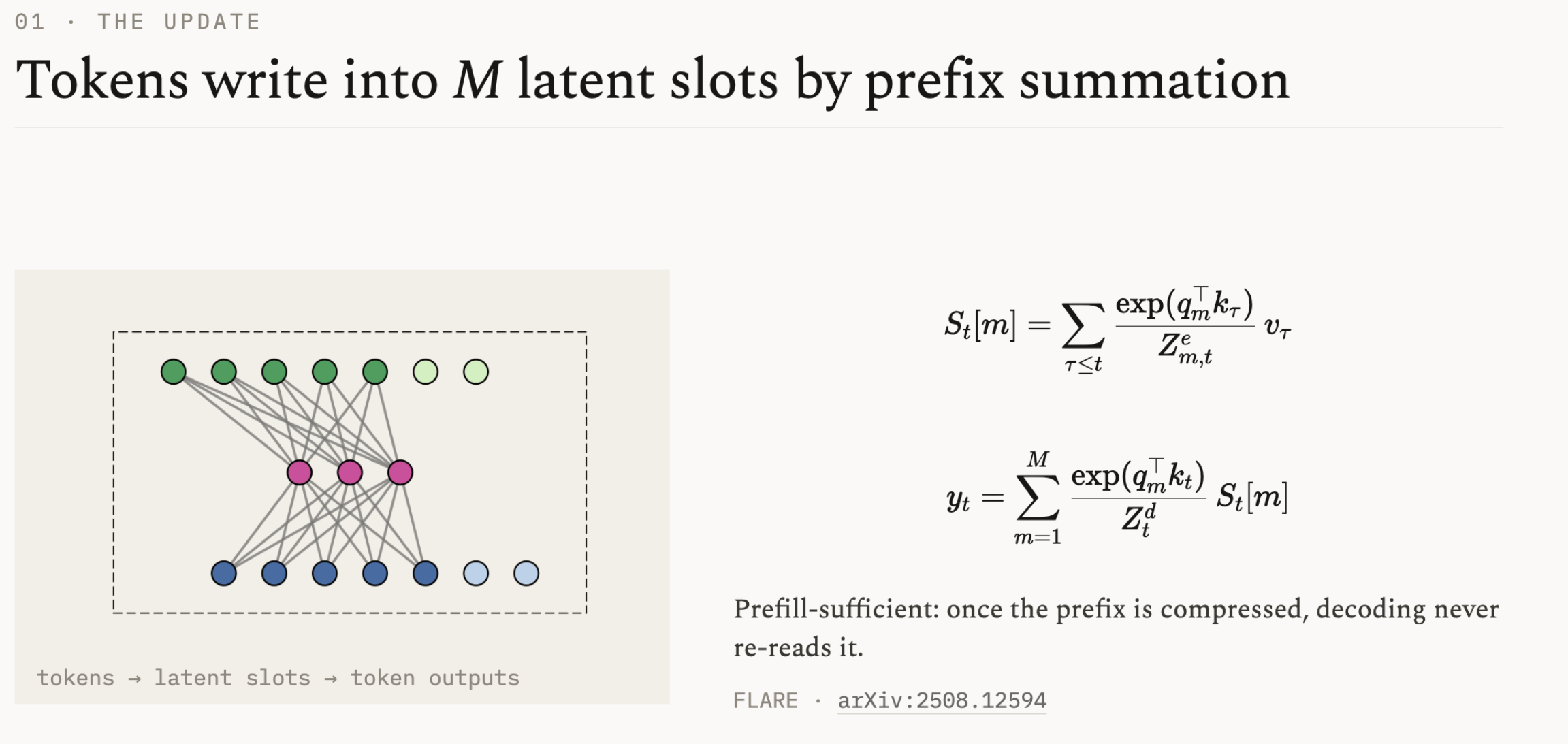
Graph weights determined by dot-product scores \(S_{m,n}=q_m^T \cdot k_n\).
Every \(\textcolor{blue}{\text{output token}}\) produces a probability distribution over \(\textcolor{green}{\text{inputs}}\).
[1] Vaswani et al. — “Attention Is All You Need”, NeurIPS 2017
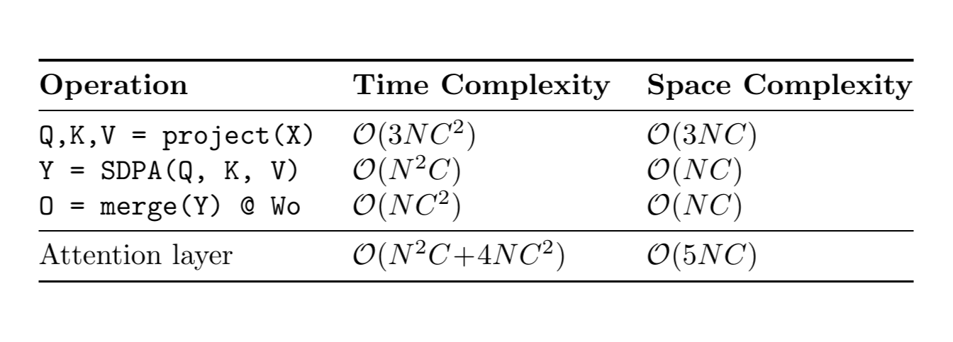
\(\mathcal{O}(N^2)\) cost of attention limits scalability
11
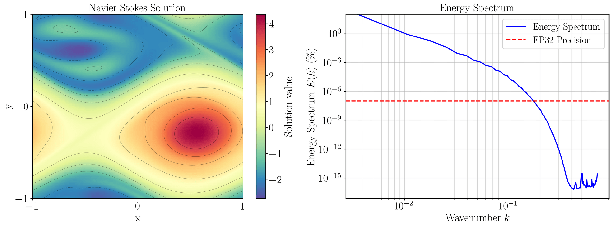
Smoothness implies redundancy in communication
\(\text{Fully-resolved flow-field}\)
11
Smoothness implies redundancy in communication
\(\text{Fully-resolved flow-field}\)
11
Smoothness implies redundancy in communication
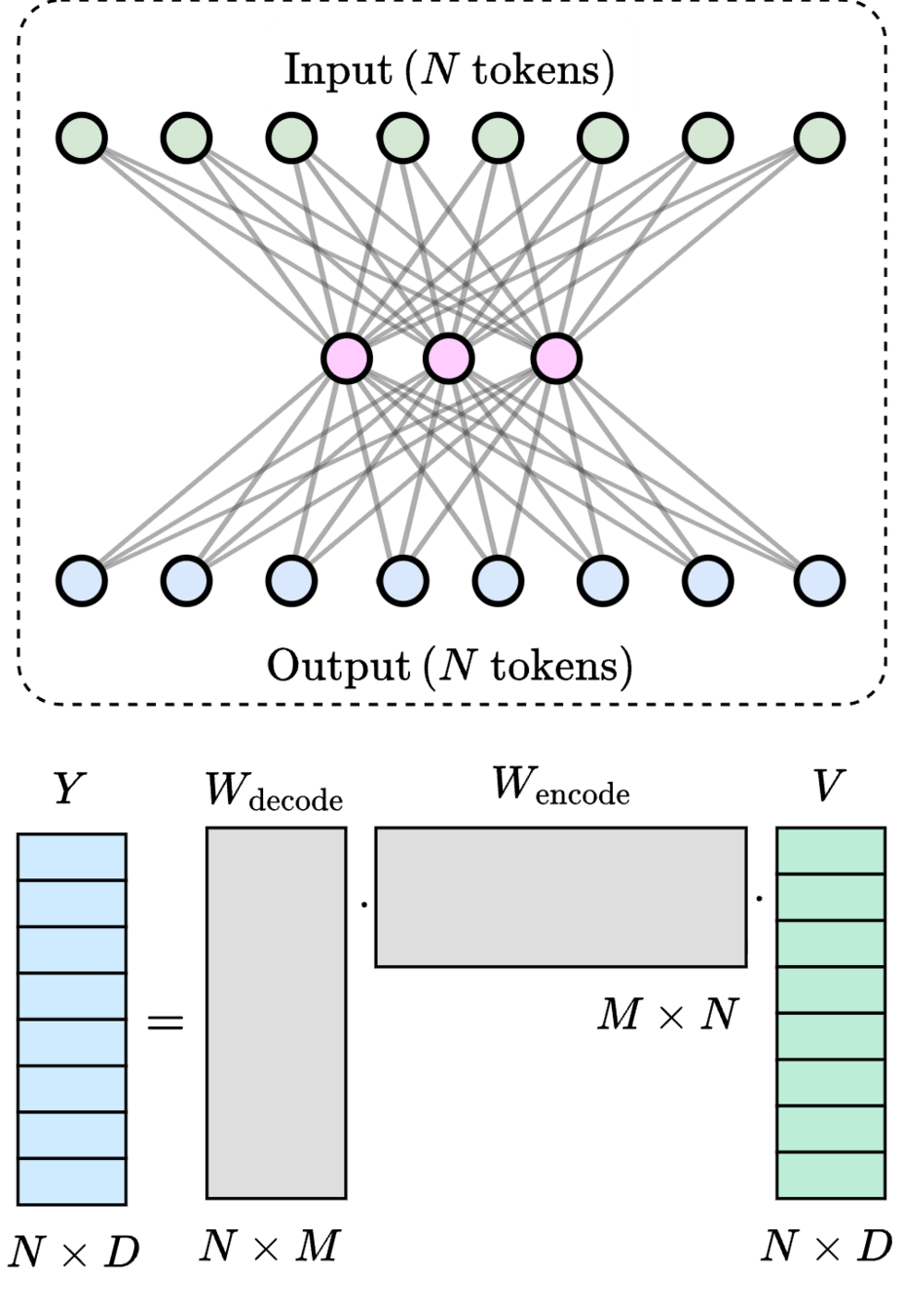
Method: club matching points to one cluster and communicate together
\(\text{Fully-resolved flow-field}\)
\(\mathcal{O}(2MN) \ll \mathcal{O}(N^2)\)
12
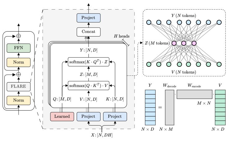
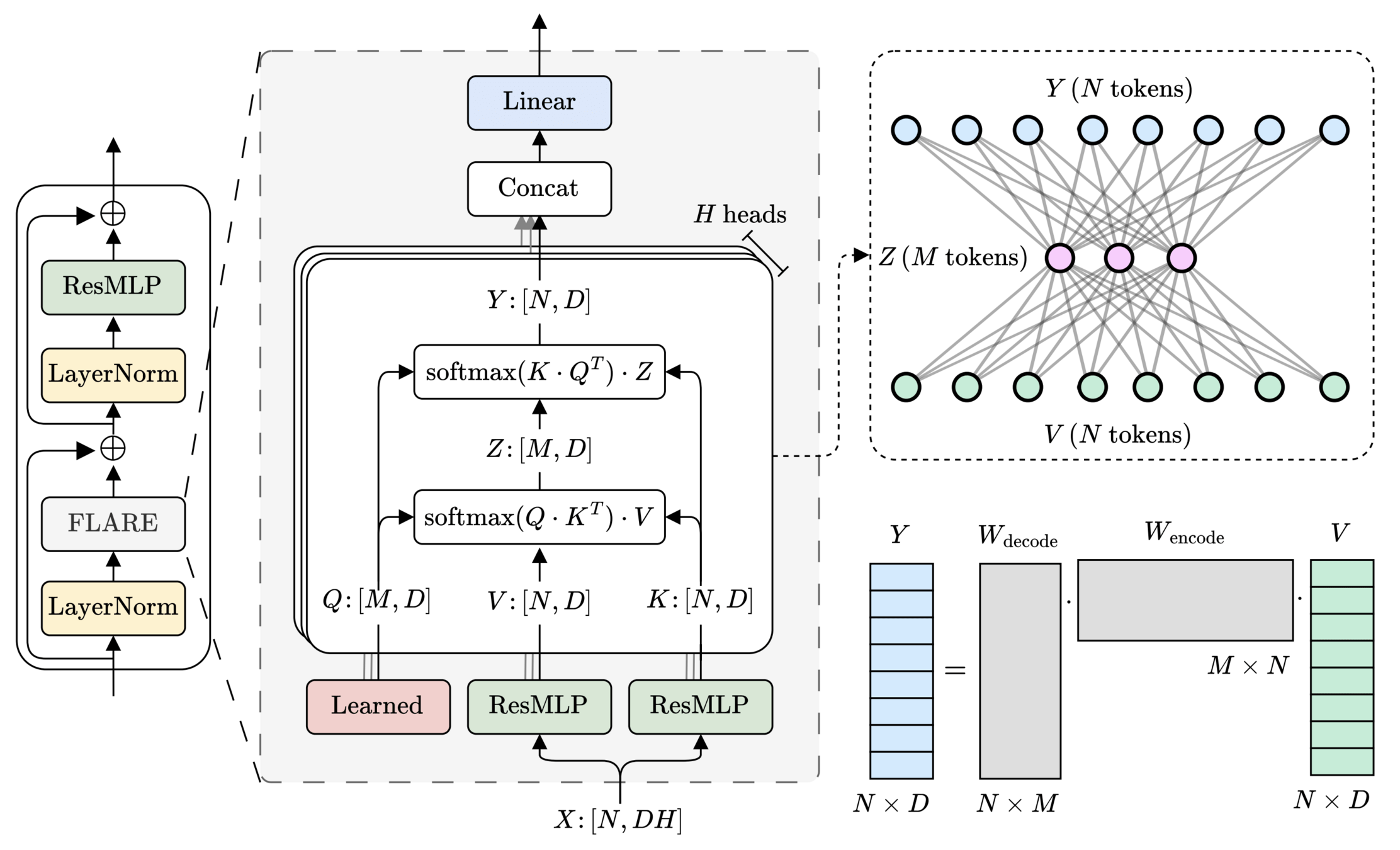
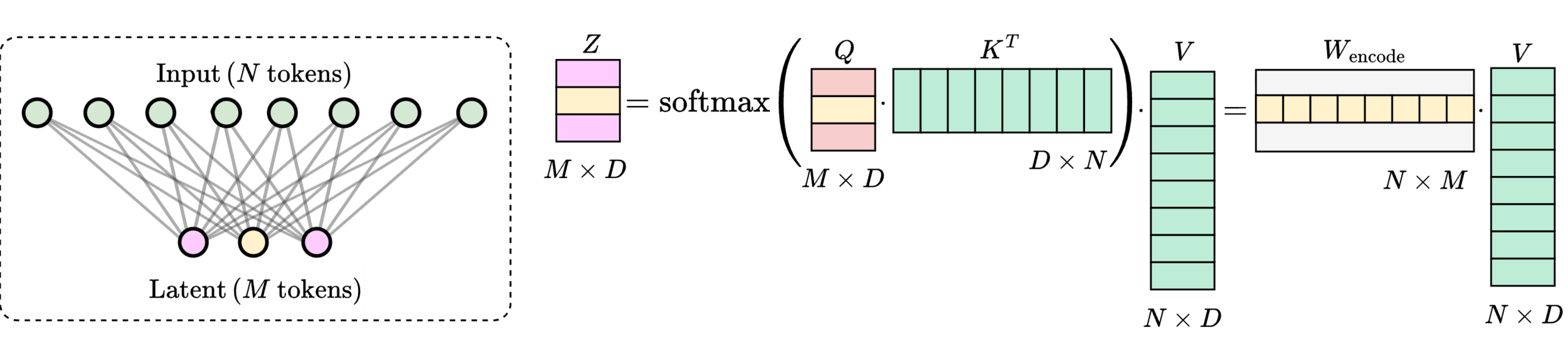
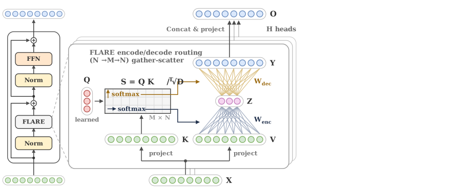
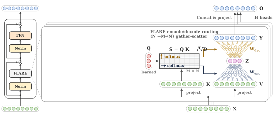
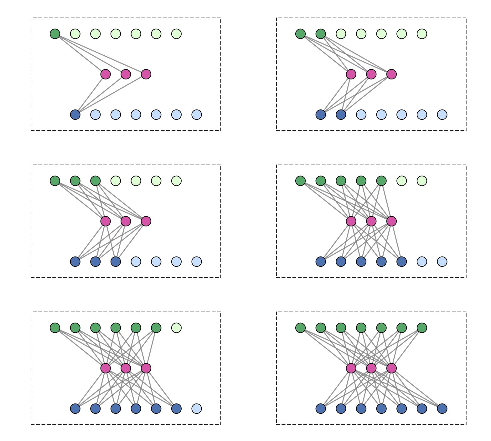
\(M\) learned queries
13
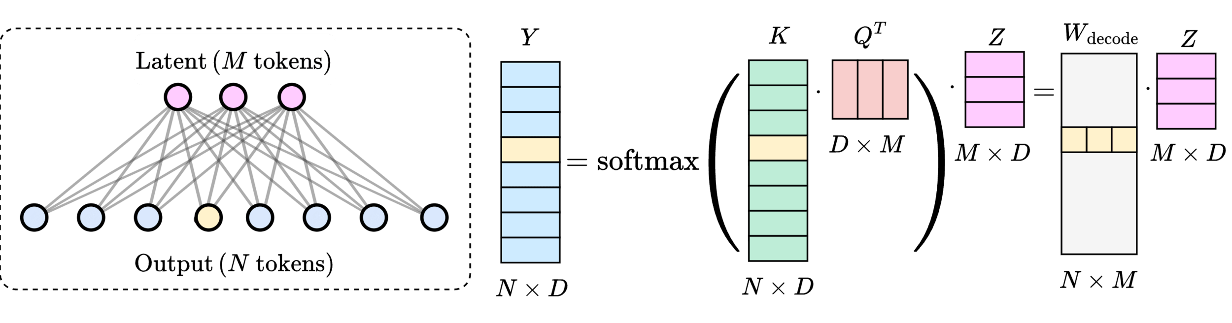
Encoding/decoding through dot-product scores against learned latents.
We use fused attention kernels.
Score matrix never truly materialized.
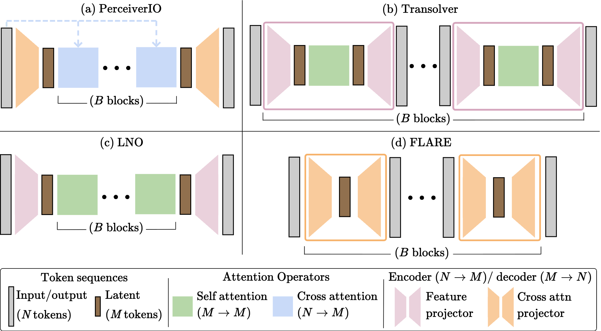
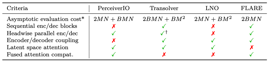
FLARE is an encode/decode
latent-space attention mechanism.
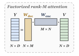
Latent-space-attention can effect factorized low-rank self-attention.
14
Simplify and connect latent-attention to low-rank self-attention
Isolate gather/scatter routing as a load-bearing primitive
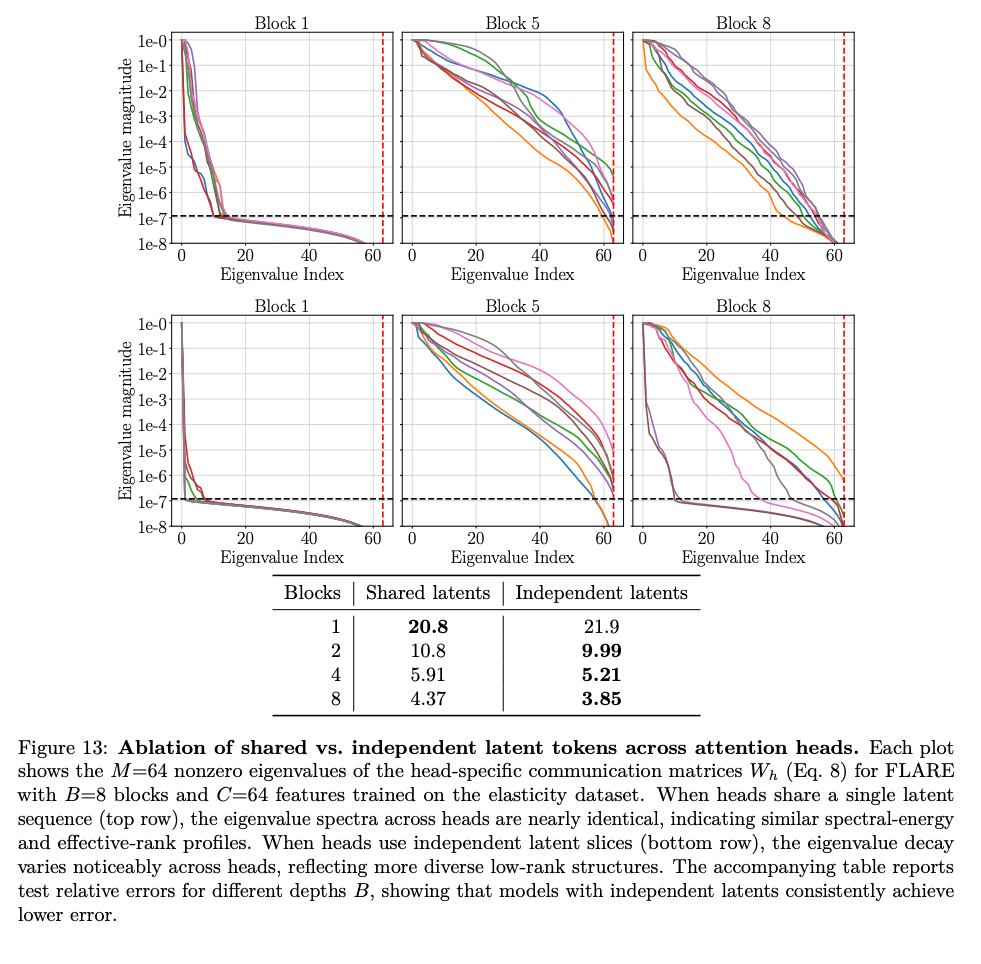
Multihead gather-scatter as parallel low-rank pathways
Each attention head learns independent latent queries
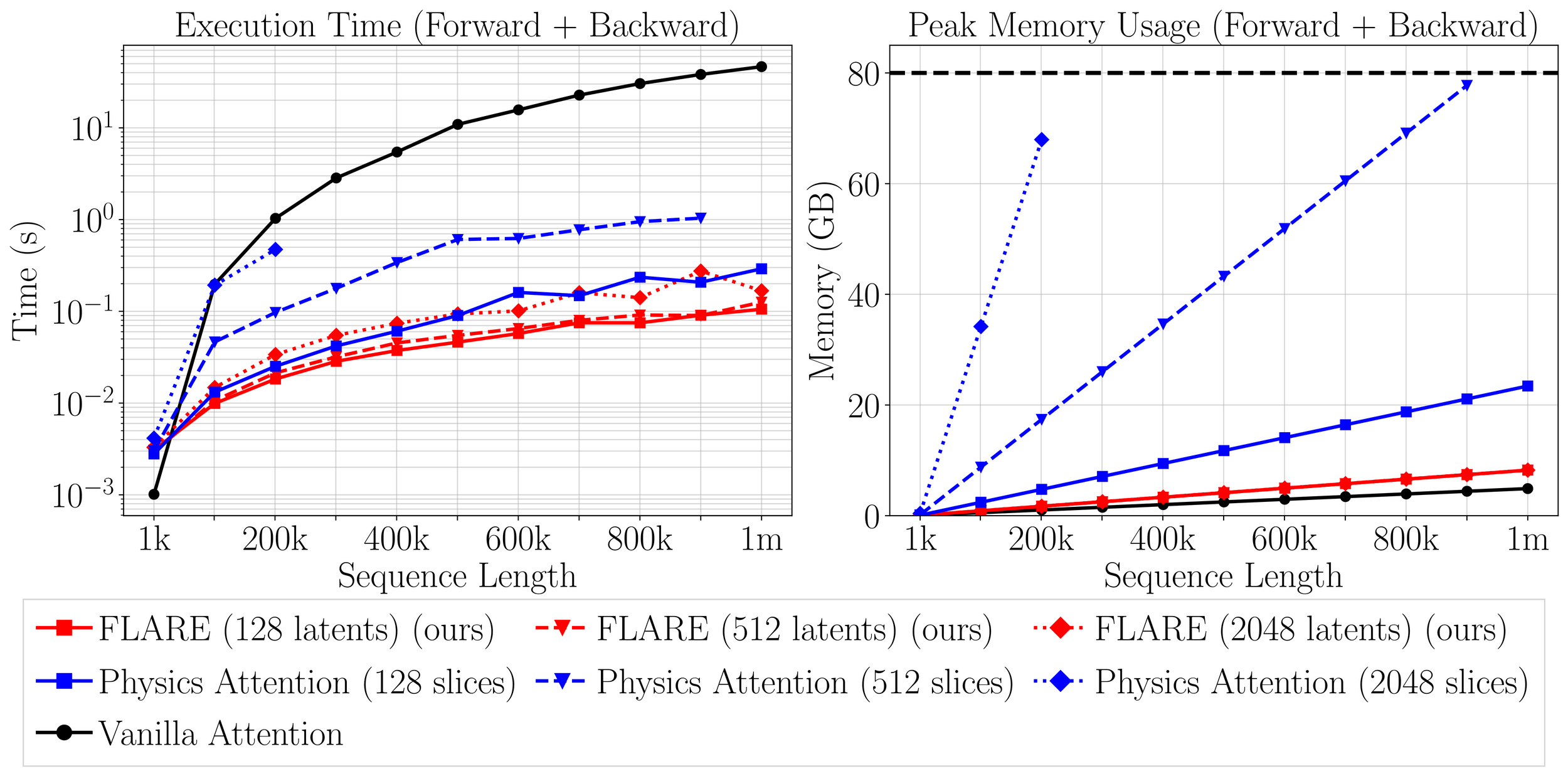
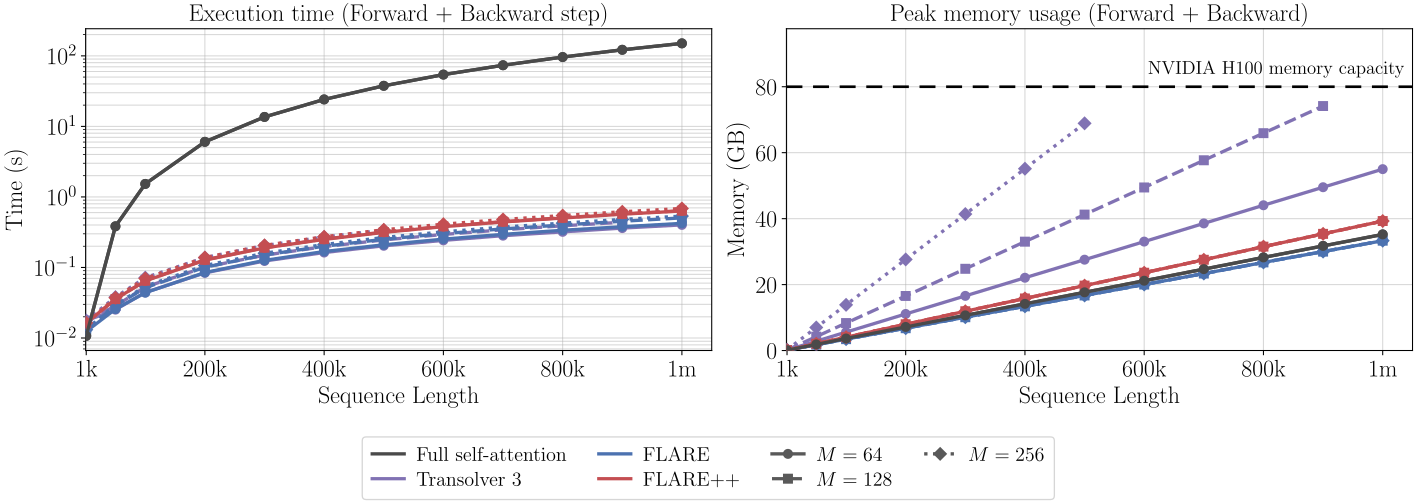
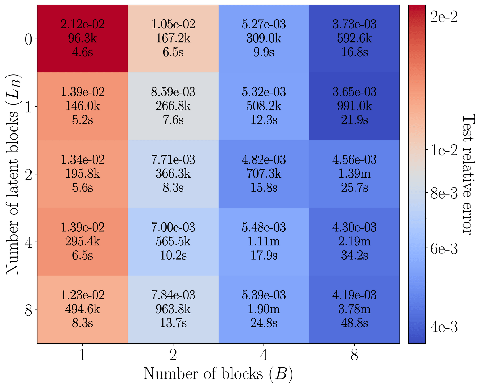
\(>200\times\) speedup over full self-attention
Extreme scalability with fused kernel implementations
Memory efficiency makes large problems tractable
15
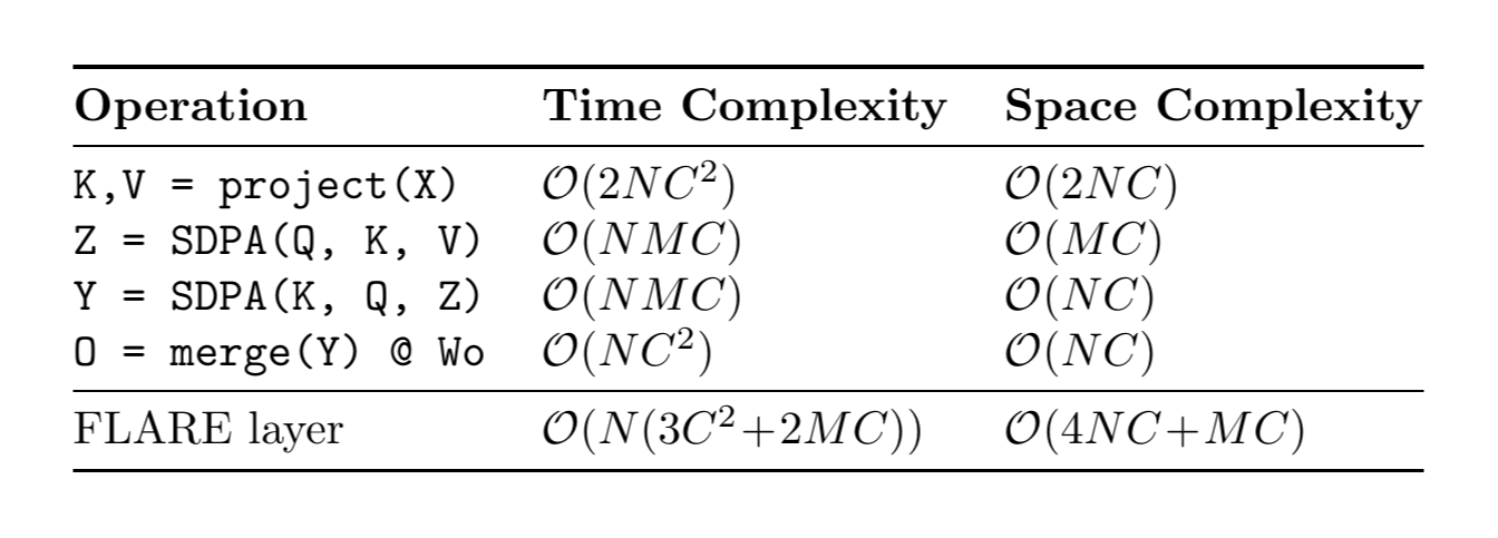
Evaluation time increases with \(M\) (\(\mathcal{O}(NMC)\))
16
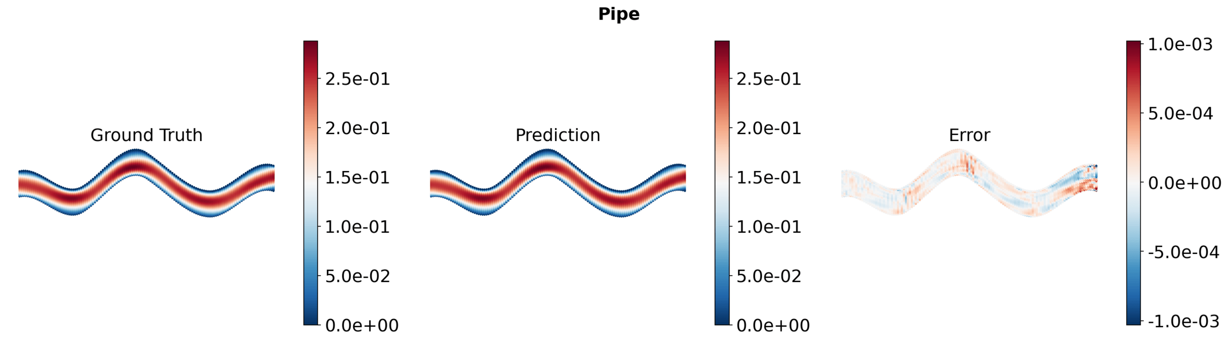
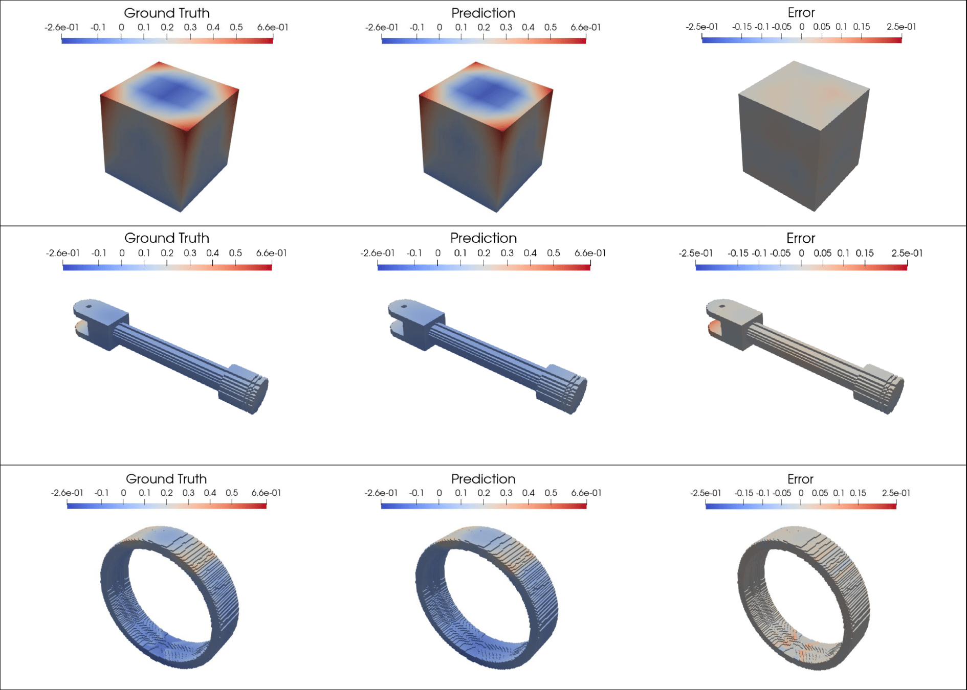
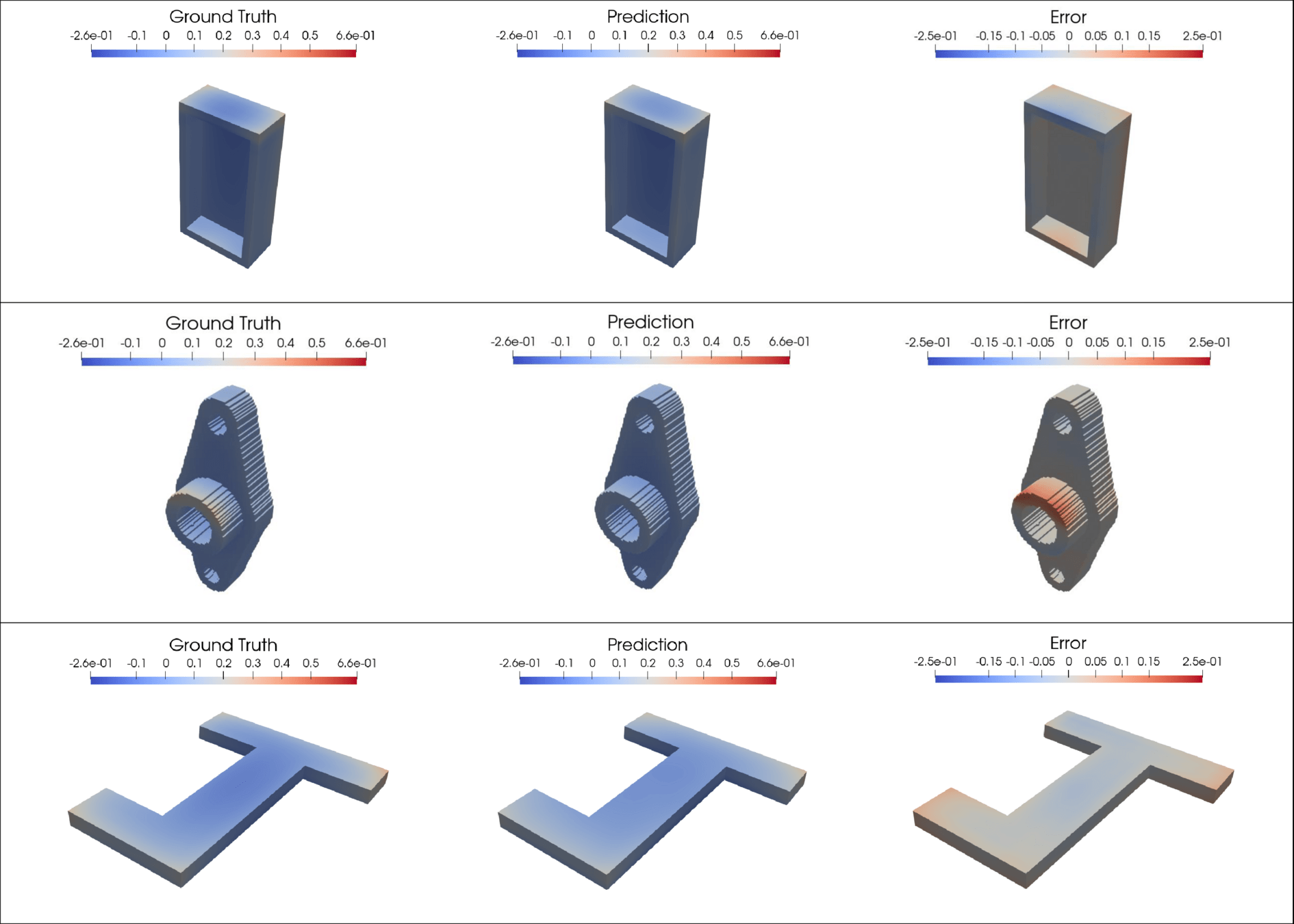
Pipe
Darcy
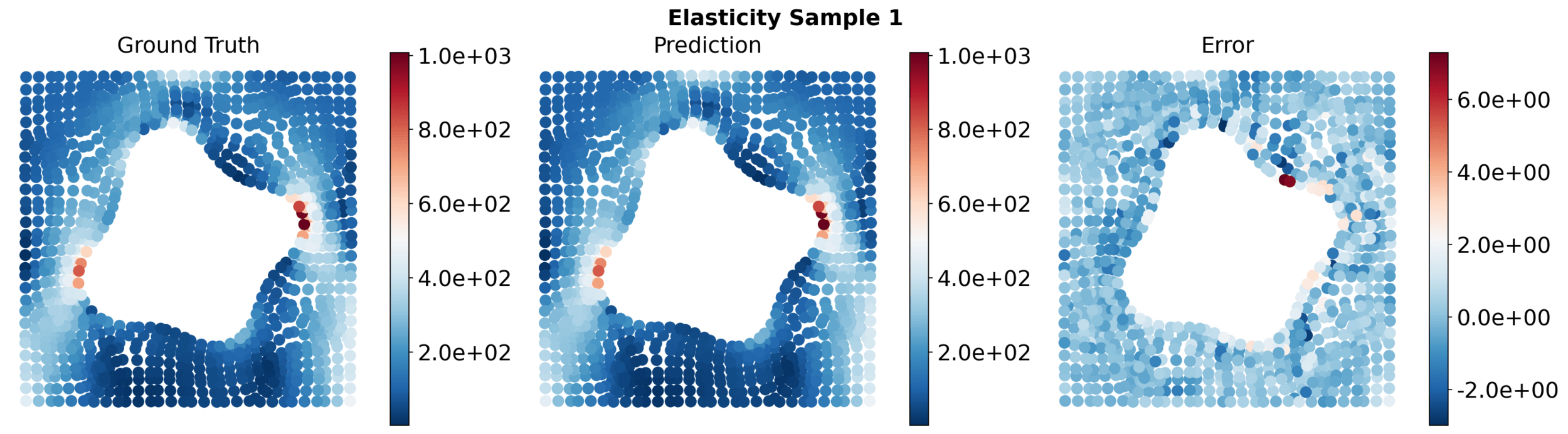
Elasticity
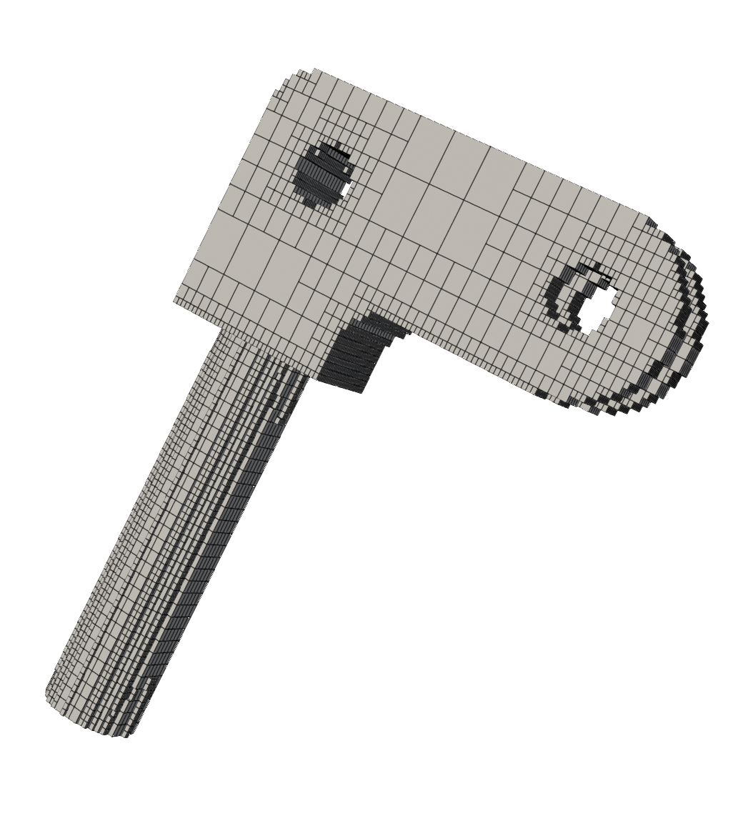
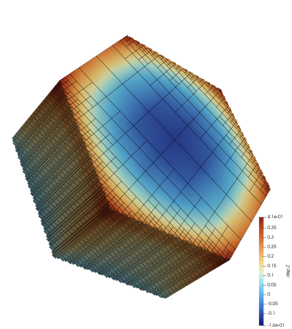
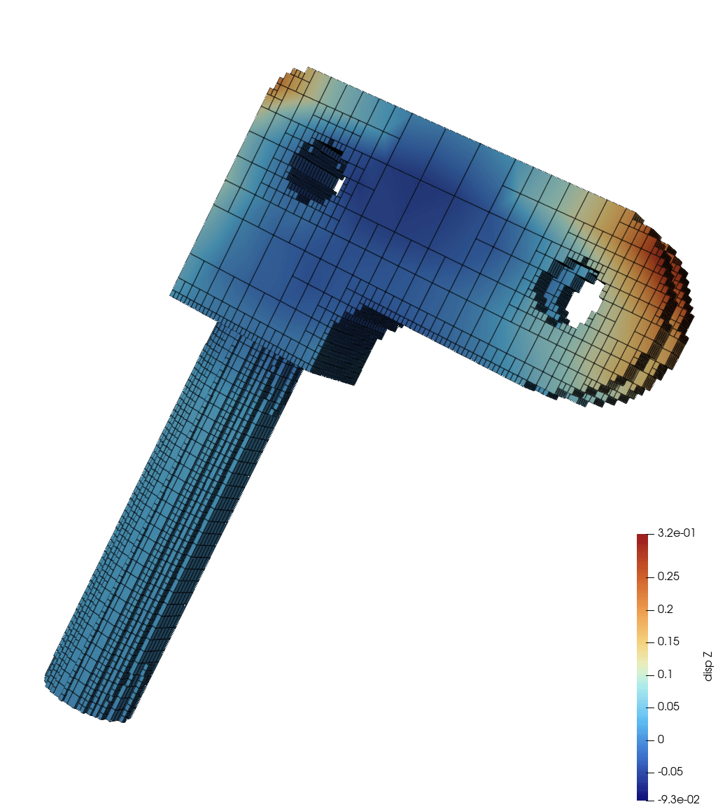
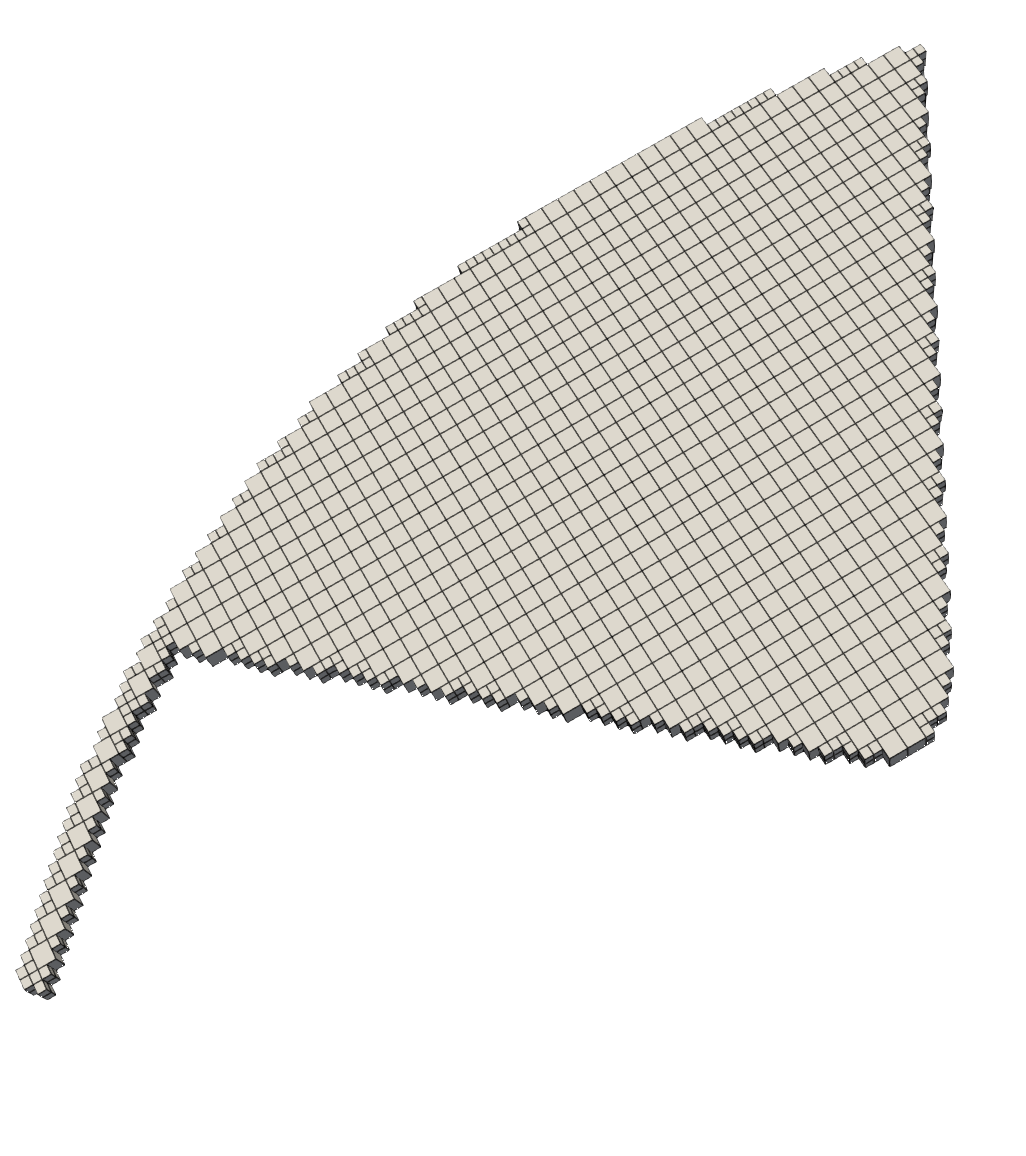
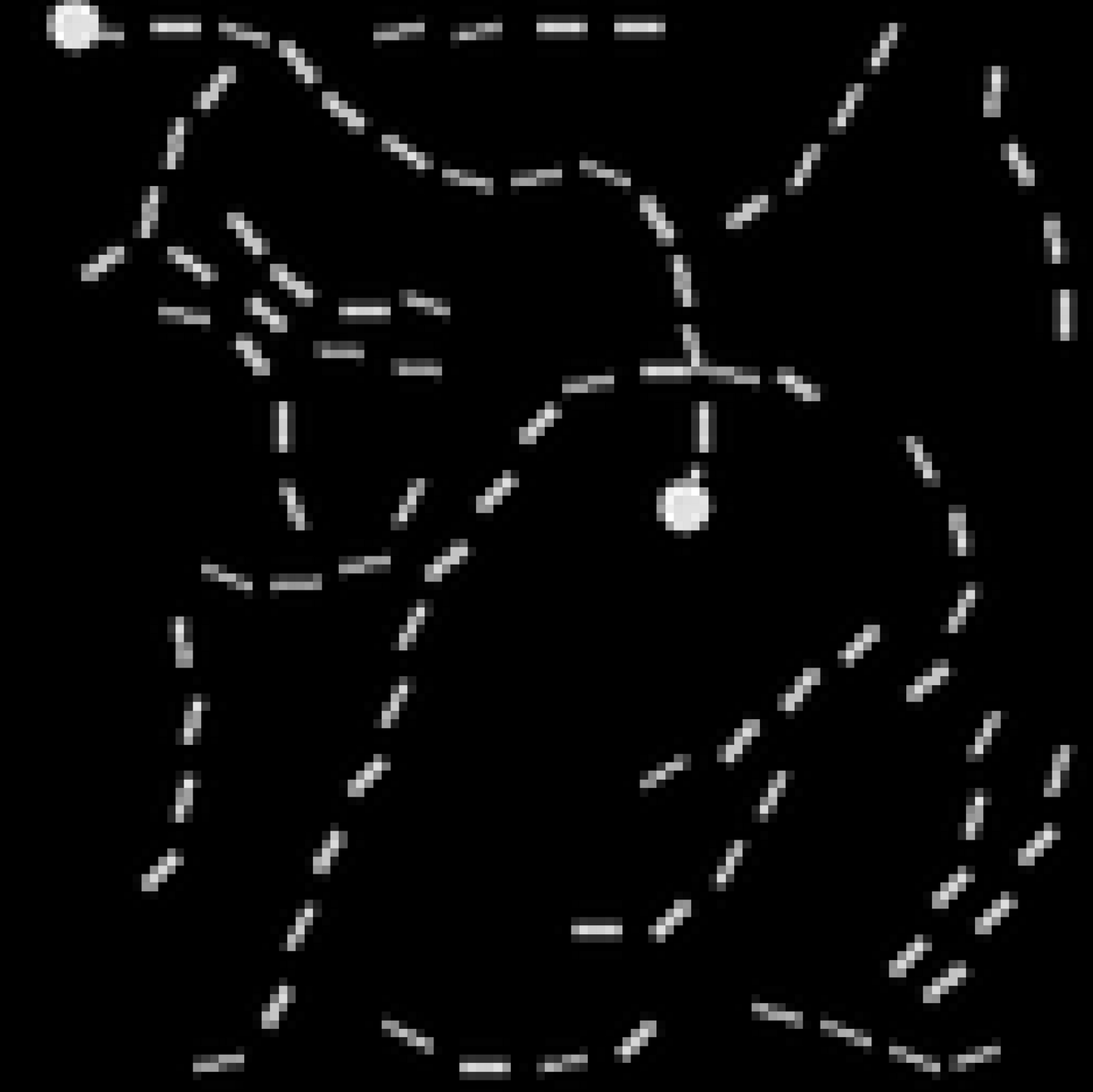
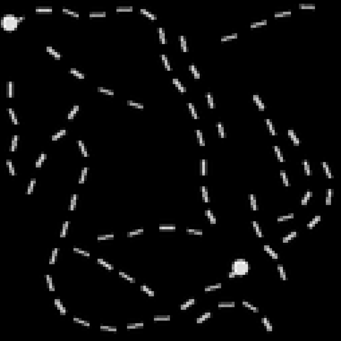
LPBF
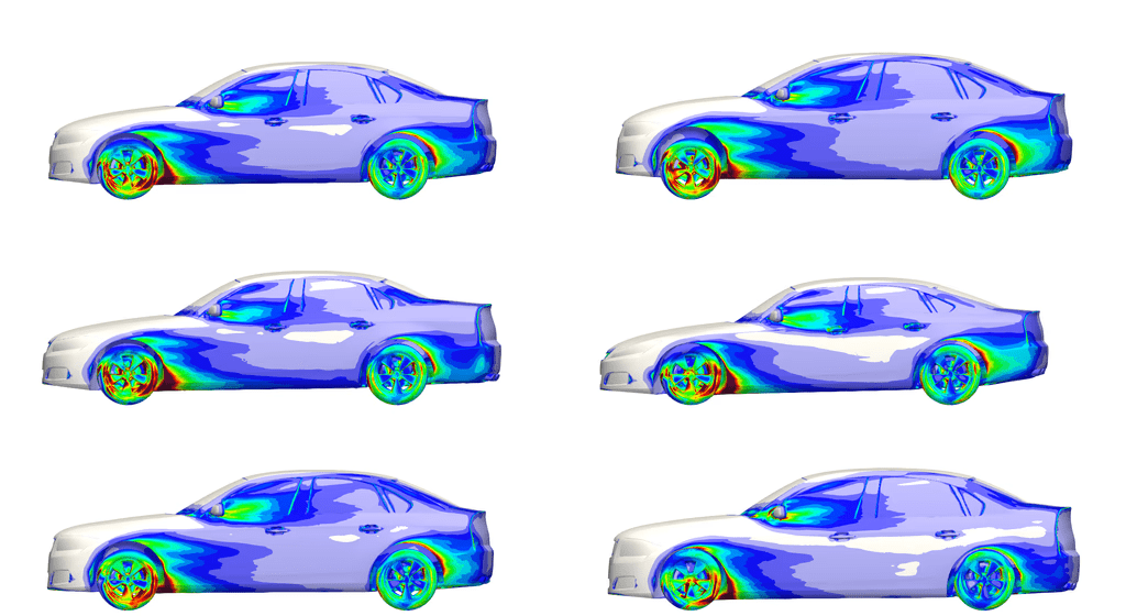
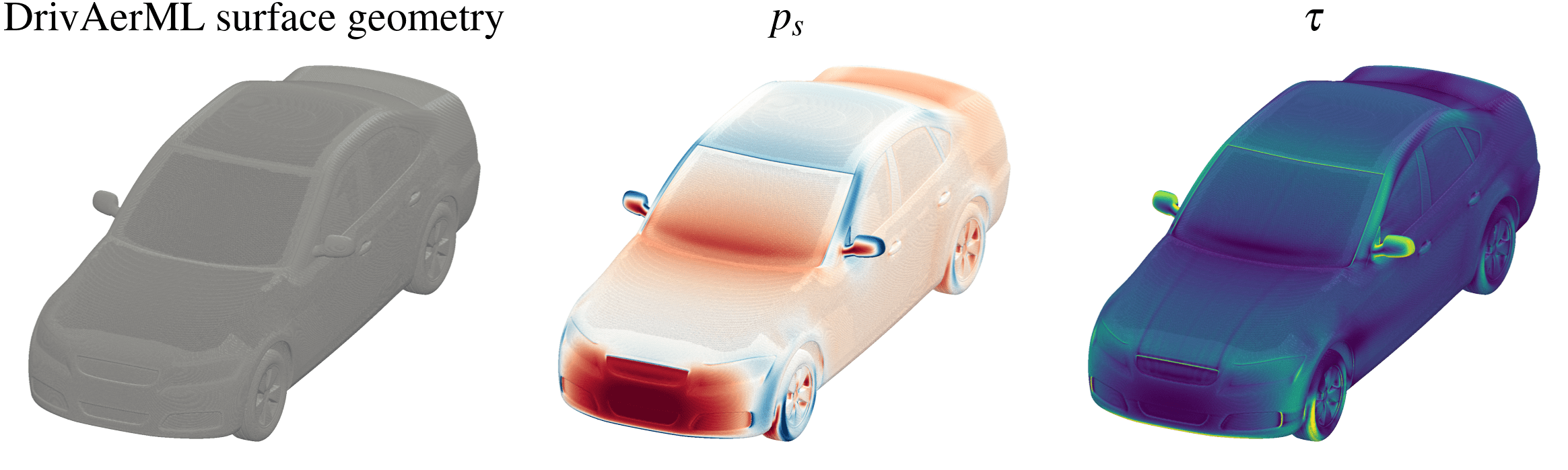
DrivAerML
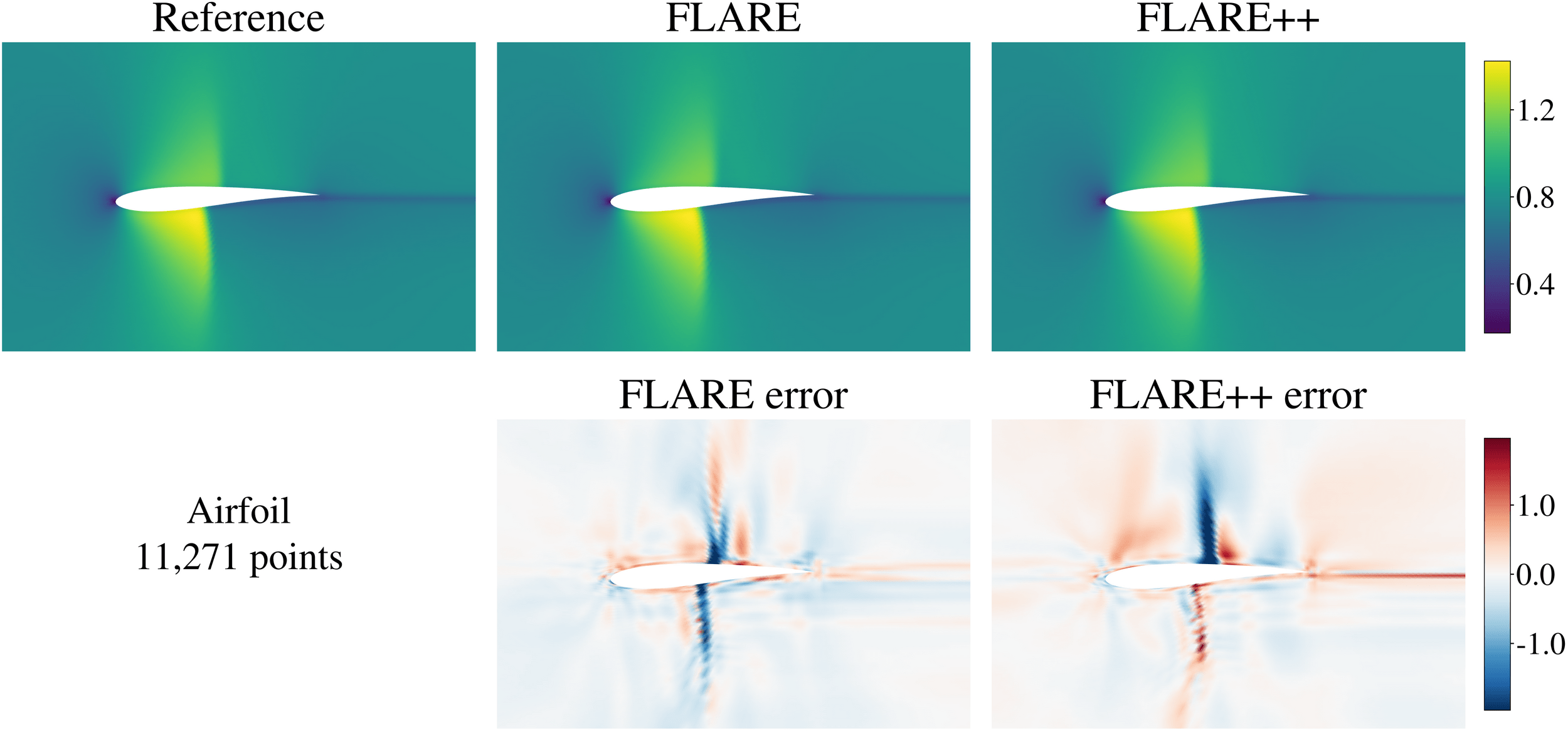
Airfoil
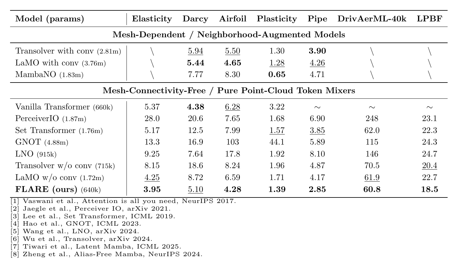
Competitive with full self-attention
Significant gains over Transolver
\(\implies\) PDE problems ok with low-rank comm.
17
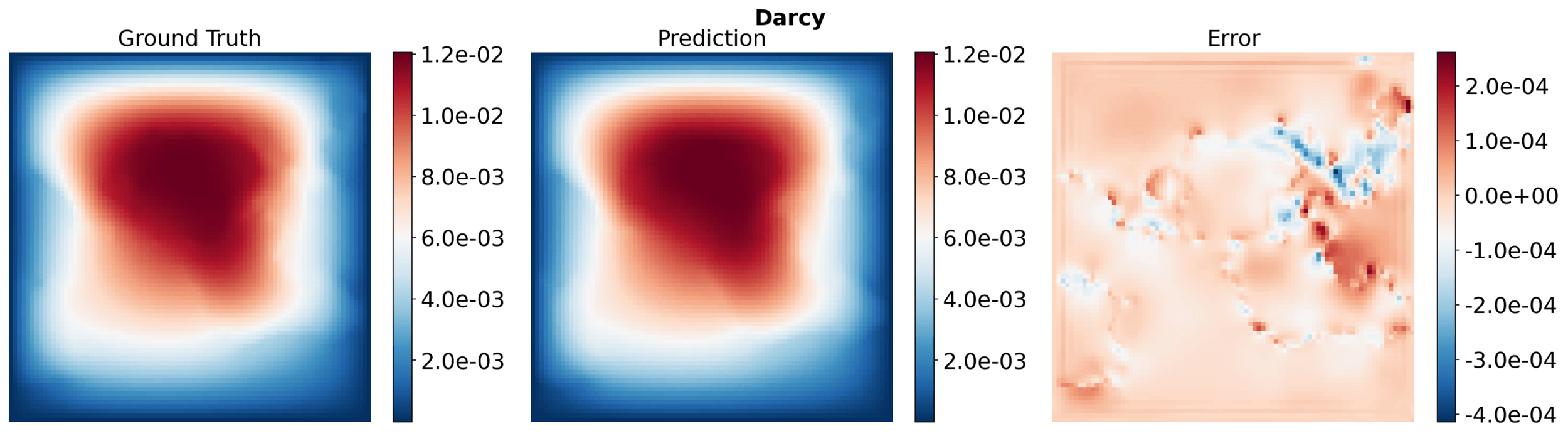
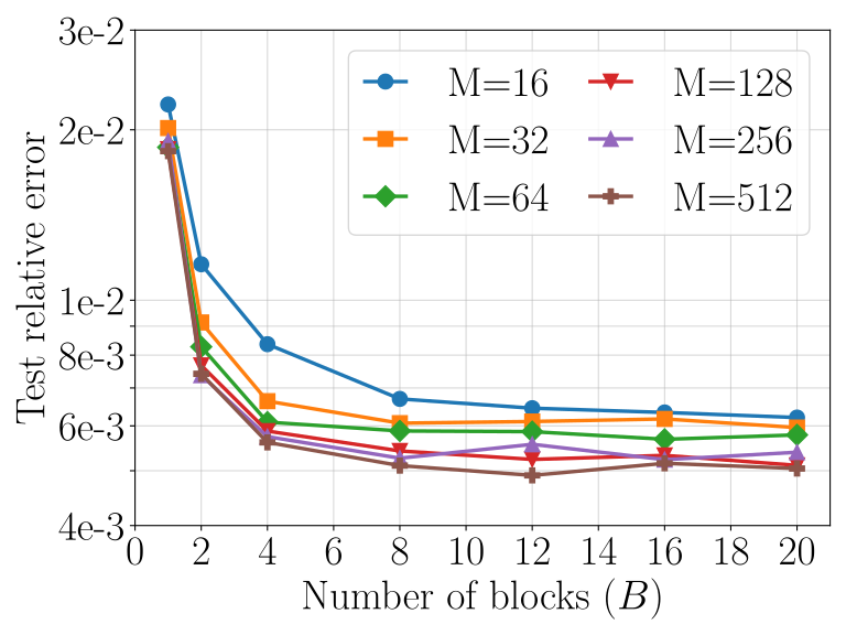
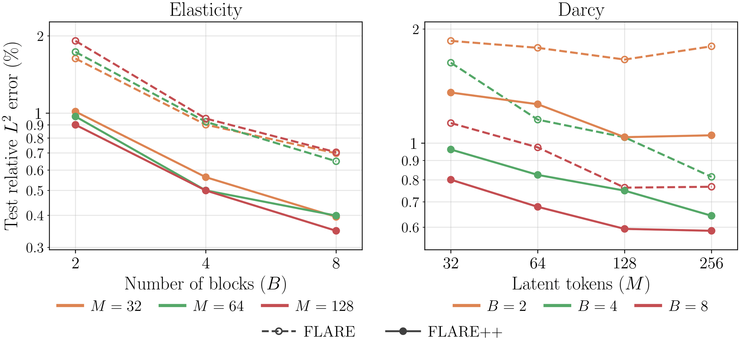
Darcy flow problem
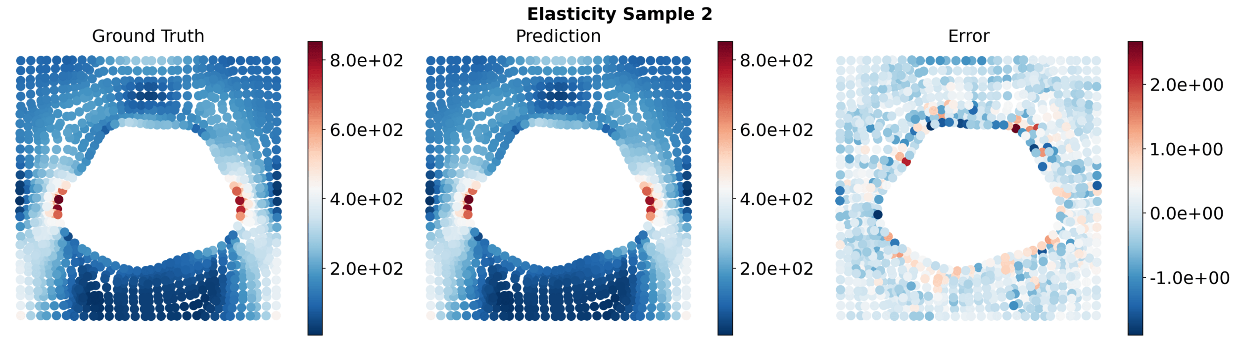
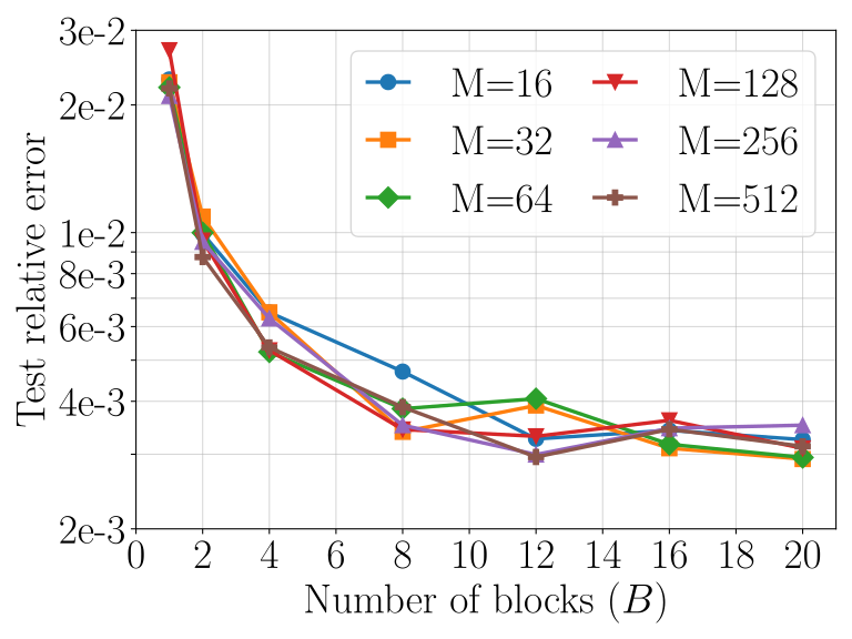
Elasticity problem
Accuracy improves with depth
Accuracy improves with \(M\) and depth!
18
\(\text{Accuracy (\%)}\)
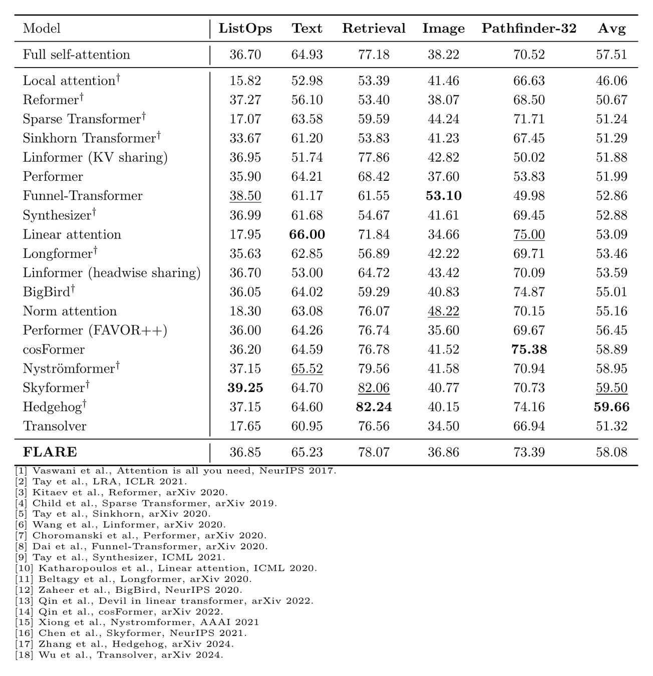
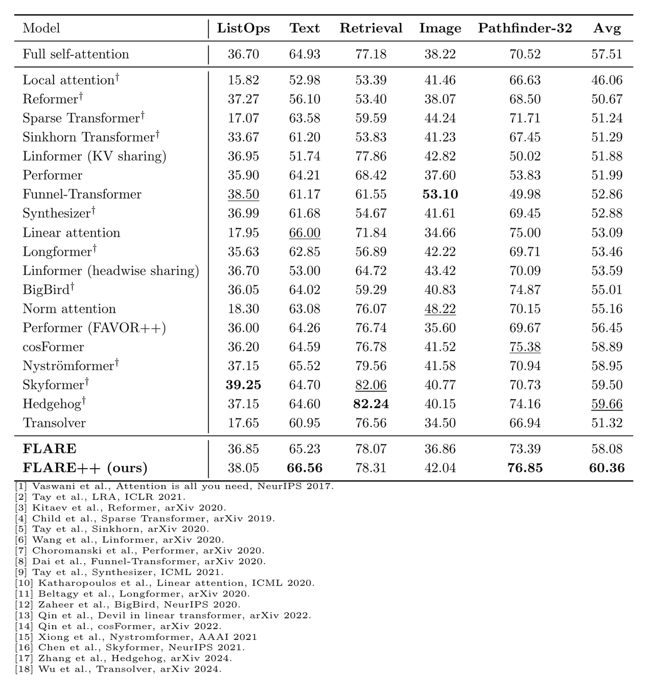
Low-rank attention generalized beyond PDE tasks
19
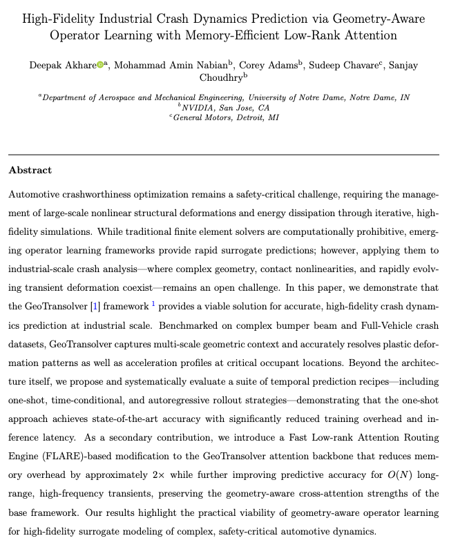
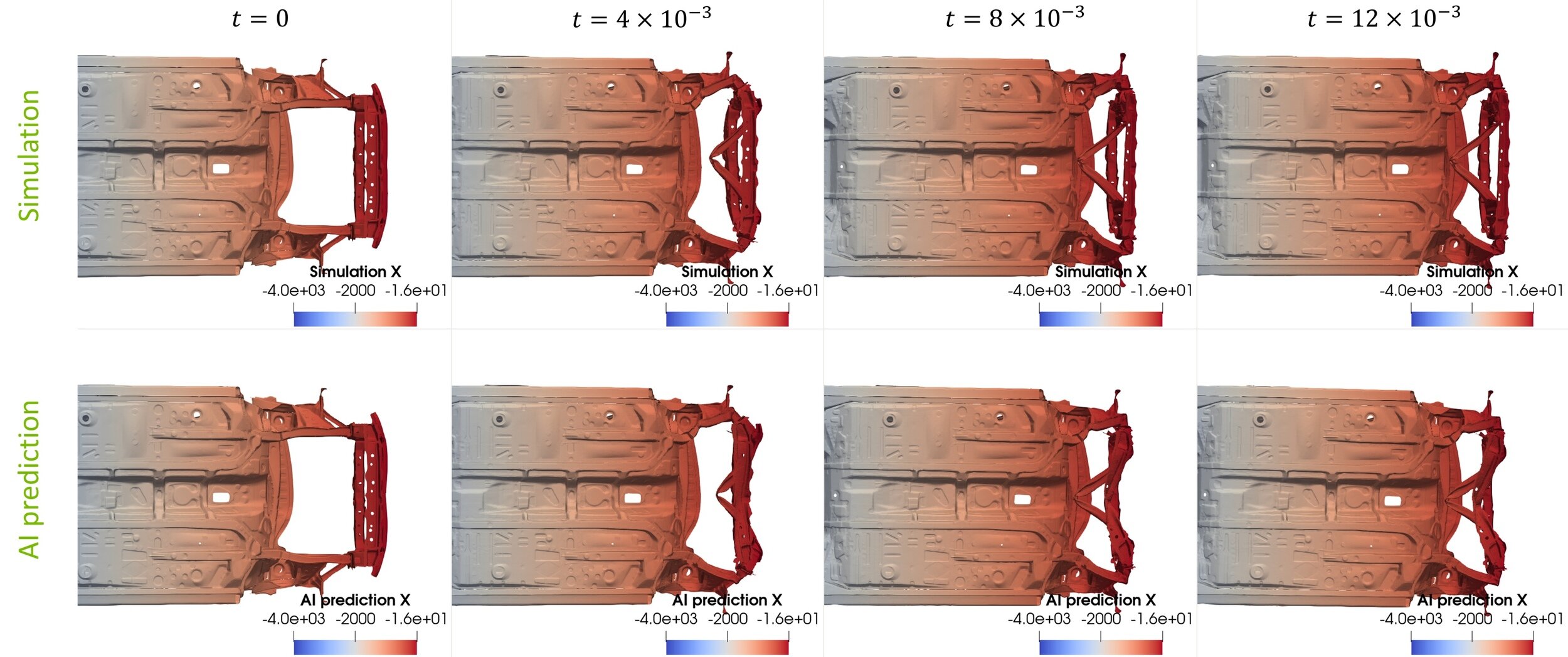
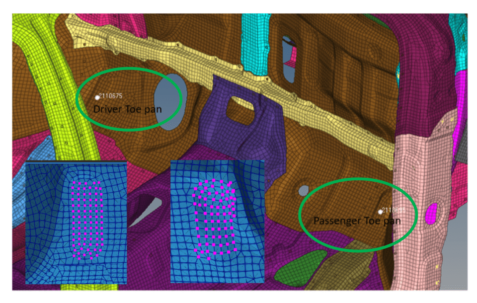
[2] Akhare et al. “High-Fidelity Industrial- Crash Dynamics”, arXiv:2605:27758
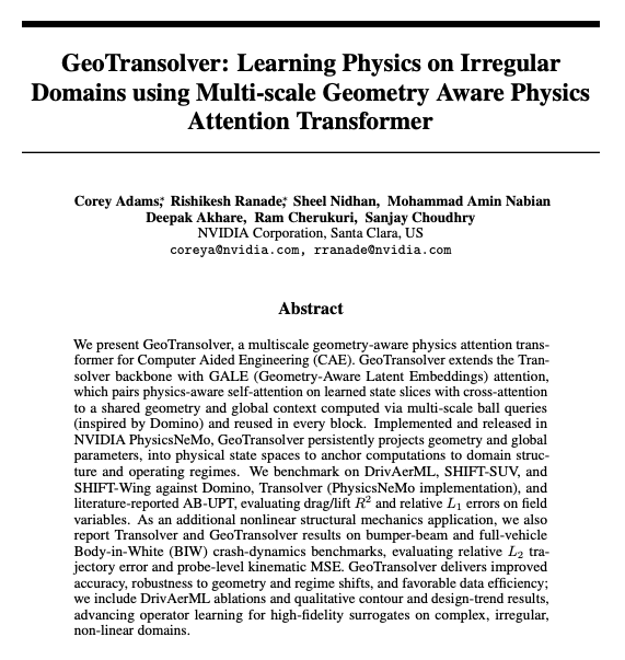
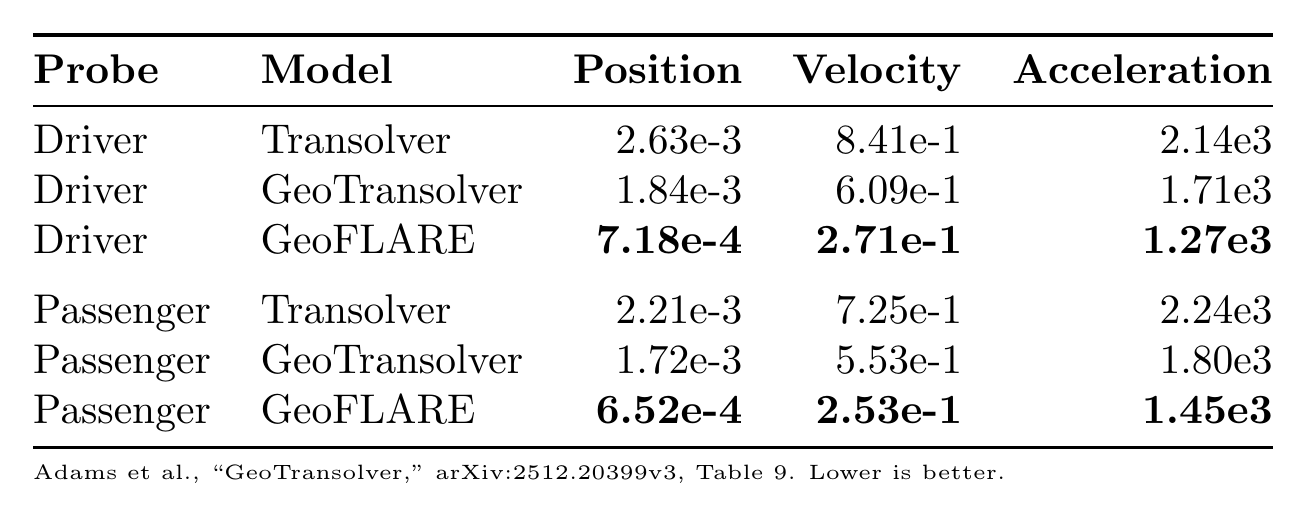
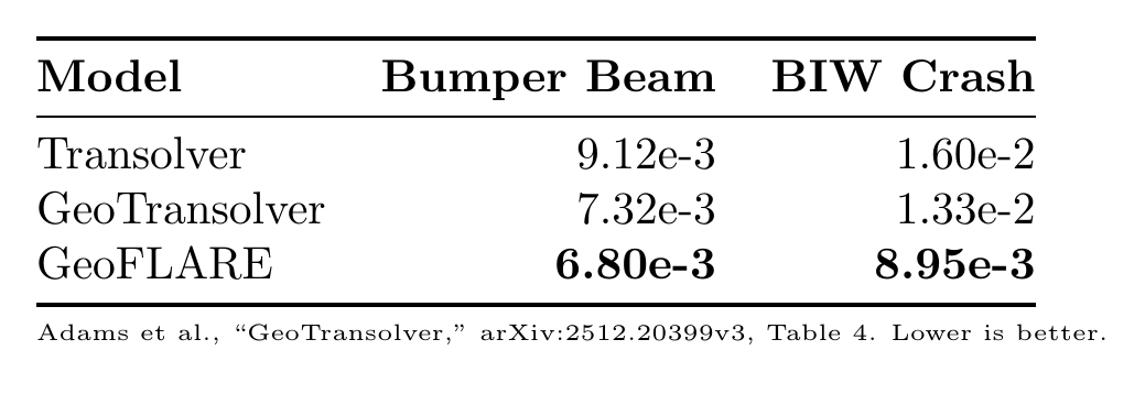
[1] Adams et al. “GeoTransolver”, arXiv:2512:20399
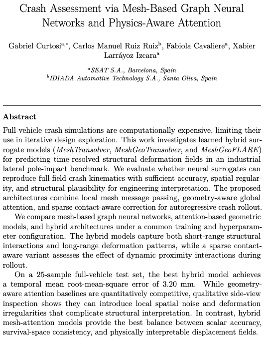
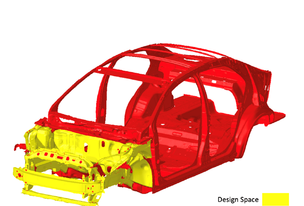
[3] Curtosi, et al. "Crash Assessment via Physics-Aware Attention", arxiv:2605:11784
Expose communication-rank as an axis of scaling
Robust and highly scalable low-rank attention model
Manuscript under review at TMLR
[1]
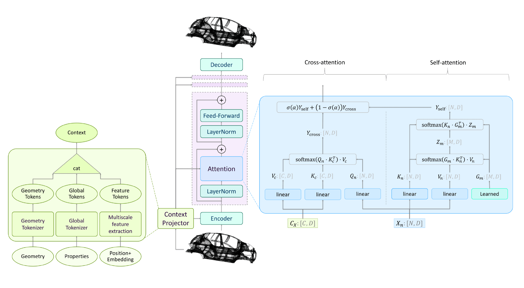
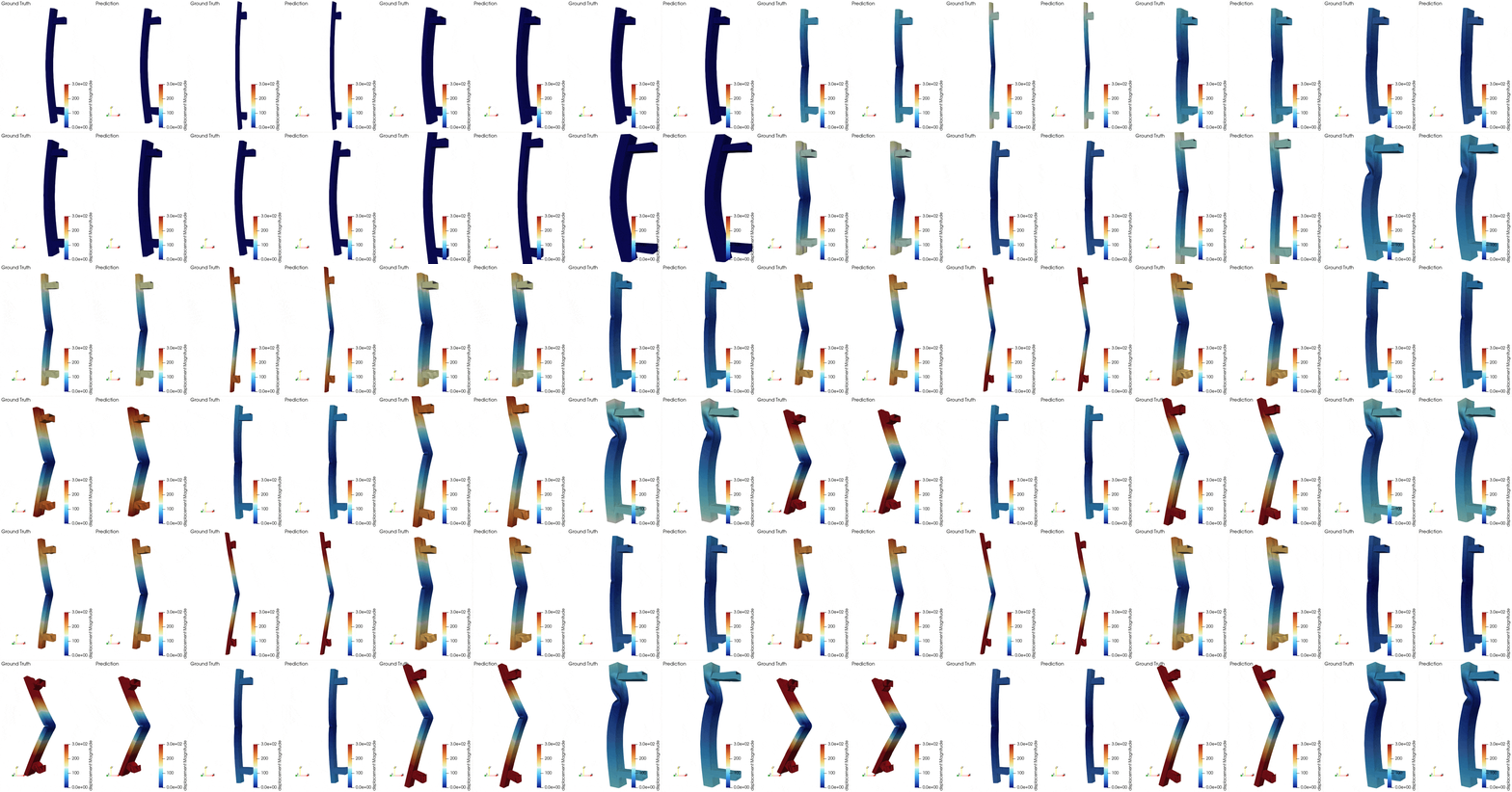
GeoFLARE: FLARE backbone + multiscale geometry feature extractor
[2]
NVIDIA
Norte Dame, GM
SEAT, IDIADA (Spain)
[3]
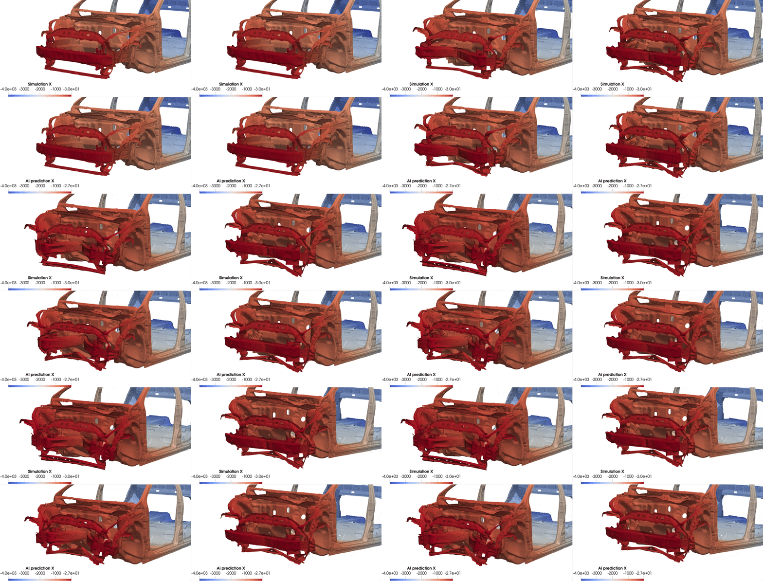
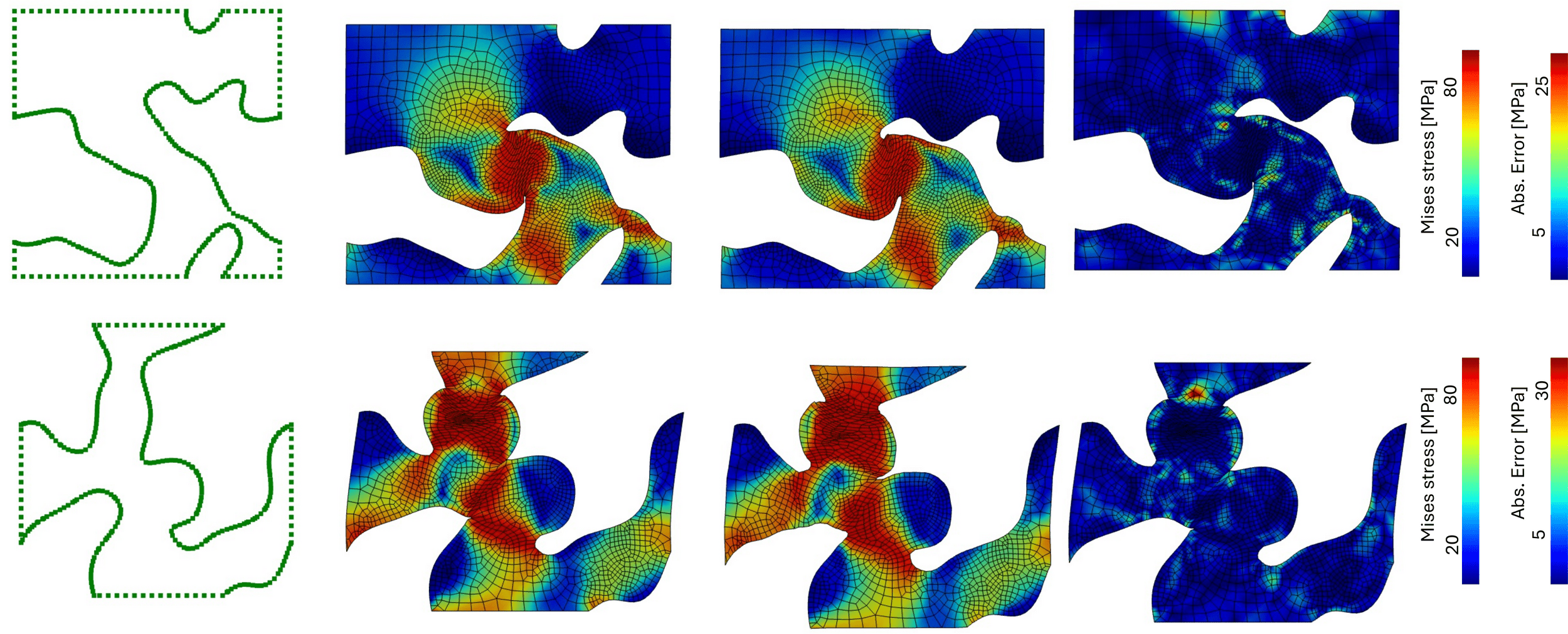
GeoFLARE on crash-dynamics problem
[2]
20
fixed, static queries.
Encode/decode weights are obtained by outer-product of input-projection with
Hypothesis: input-dependent queries can improve accuracy
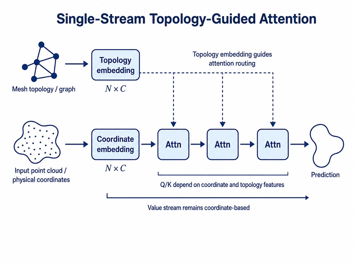
\(S_{m,n}(X) = q_m^T \cdot k_n(X)\)
20
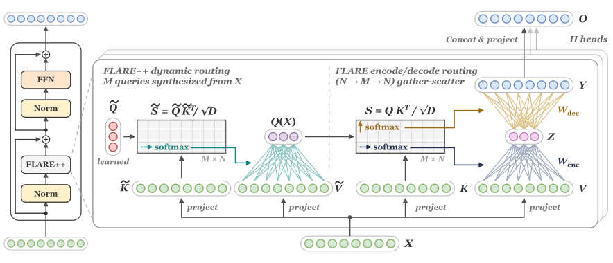
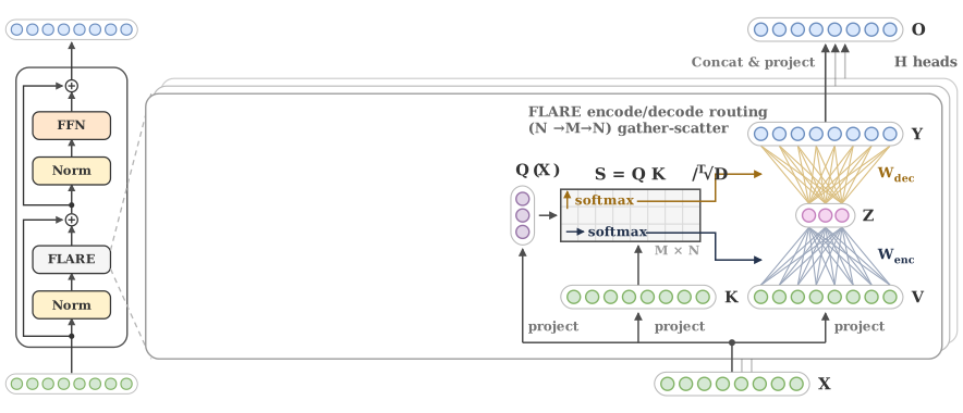
How to produce \(M\) latents from \(N\) inputs?
fixed, static queries.
Hypothesis: more expressive scores can improve accuracy
Encode/decode weights are obtained by outer-product of input-projection with
\(S_{m,n}(X) = q_m^T \cdot k_n(X)\)
20
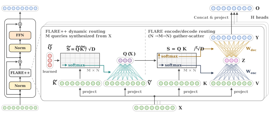
input-dependent queries.
Dynamic query synthesis
via FLARE encoder
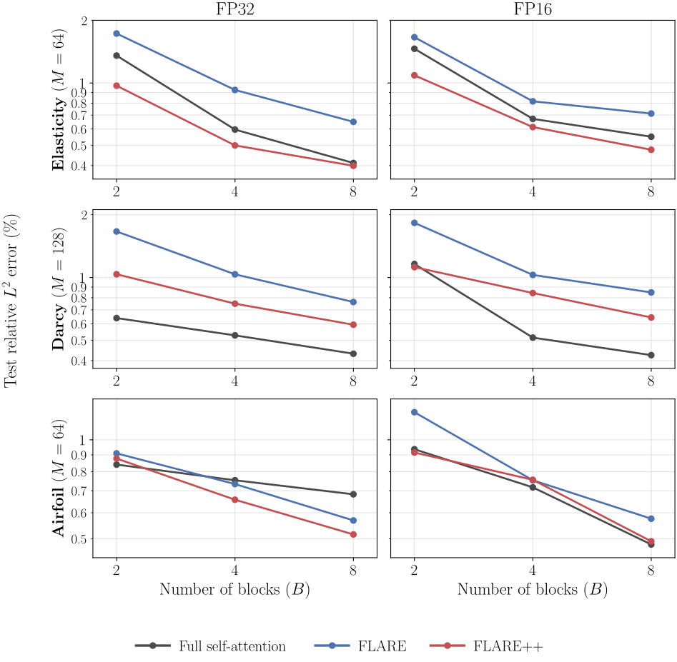
FLARE++ has \(30\%\) more params.
The output stream is intact.
All gains from improved routing.
Hypothesis: more expressive scores can improve accuracy
Encode/decode weights are obtained by outer-product of input-projection with
\(S_{m,n}(X) = q_m^T(X) \cdot k_n(X)\)
21
Pipe
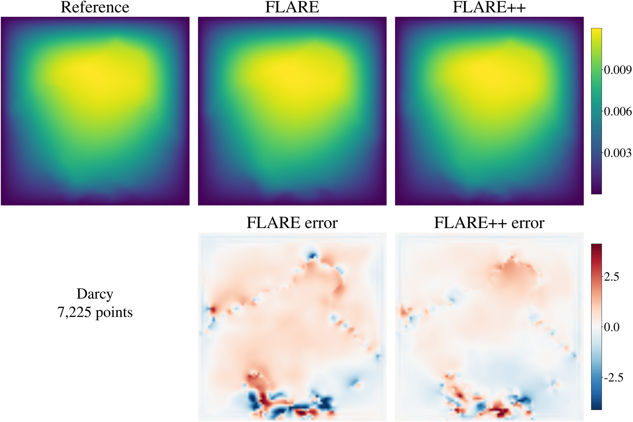
Darcy
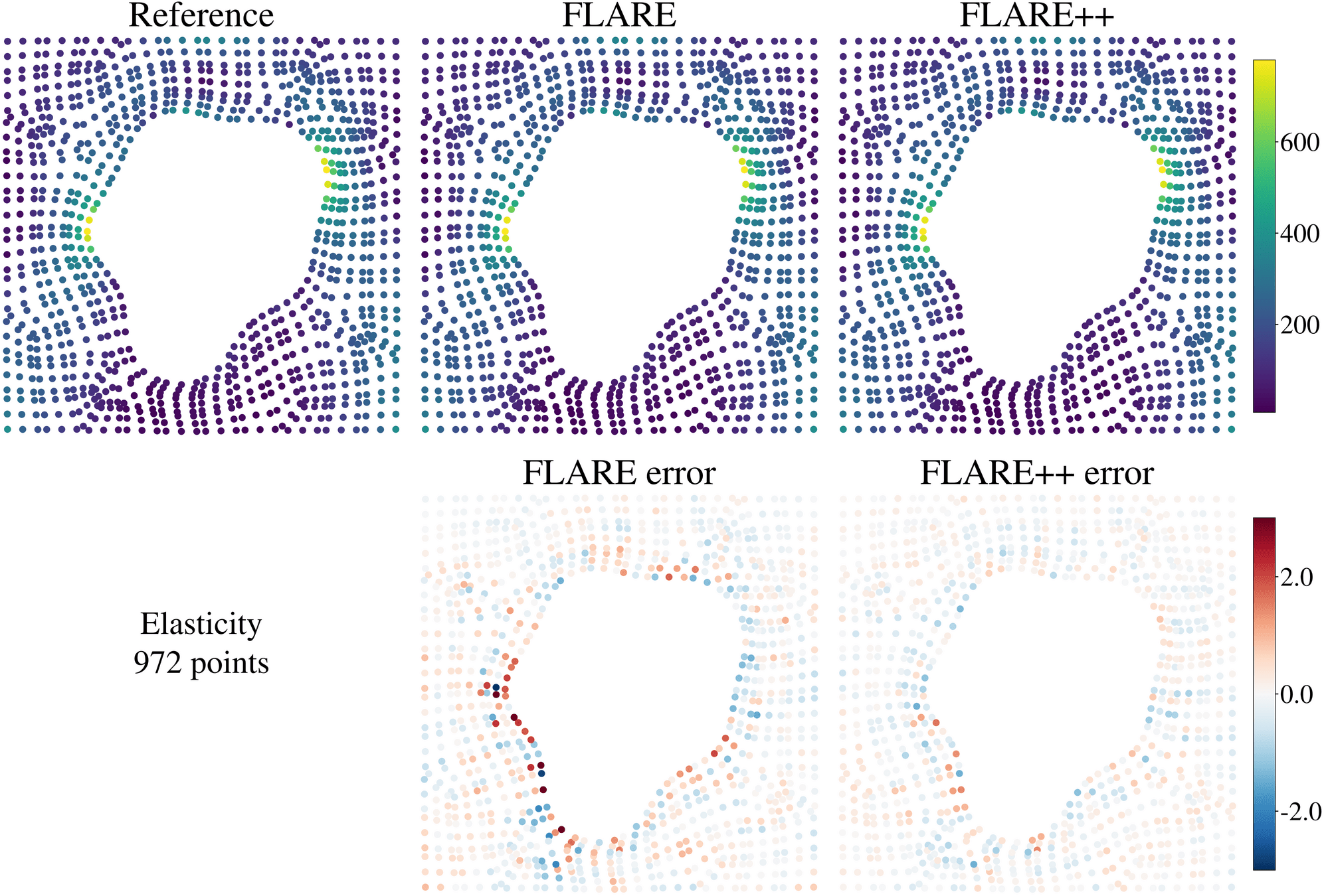
Elasticity
DrivAerML
Airfoil
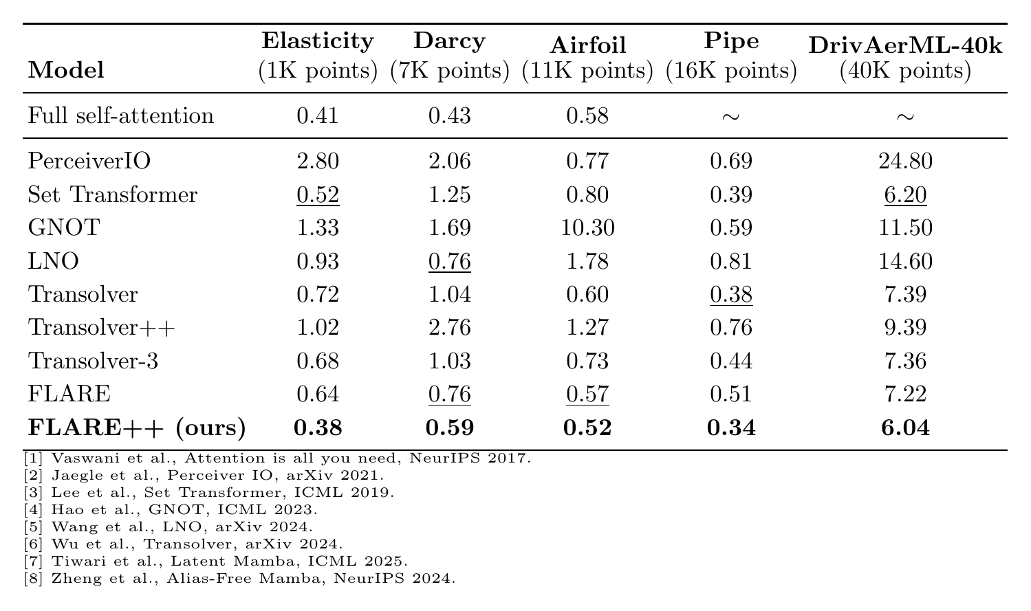
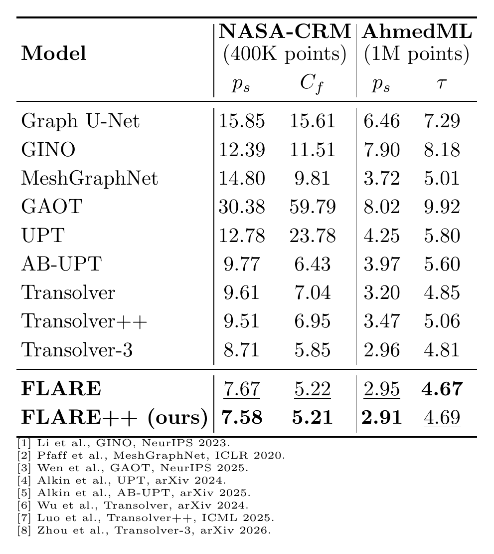
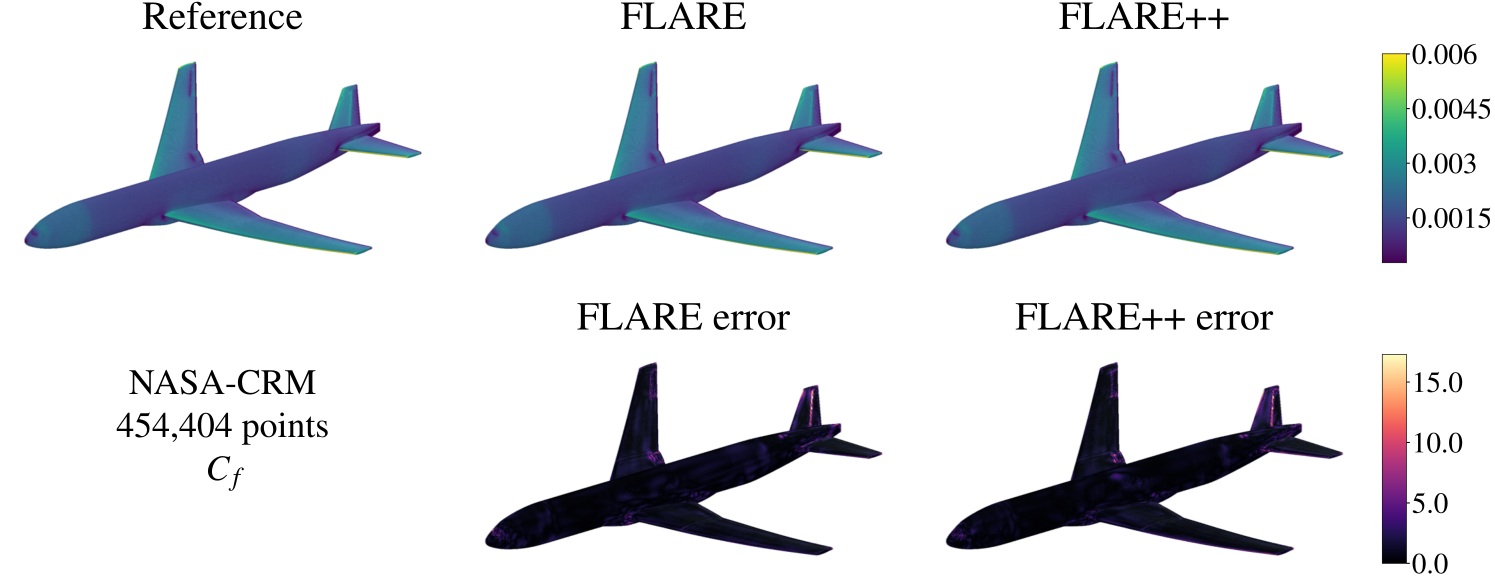
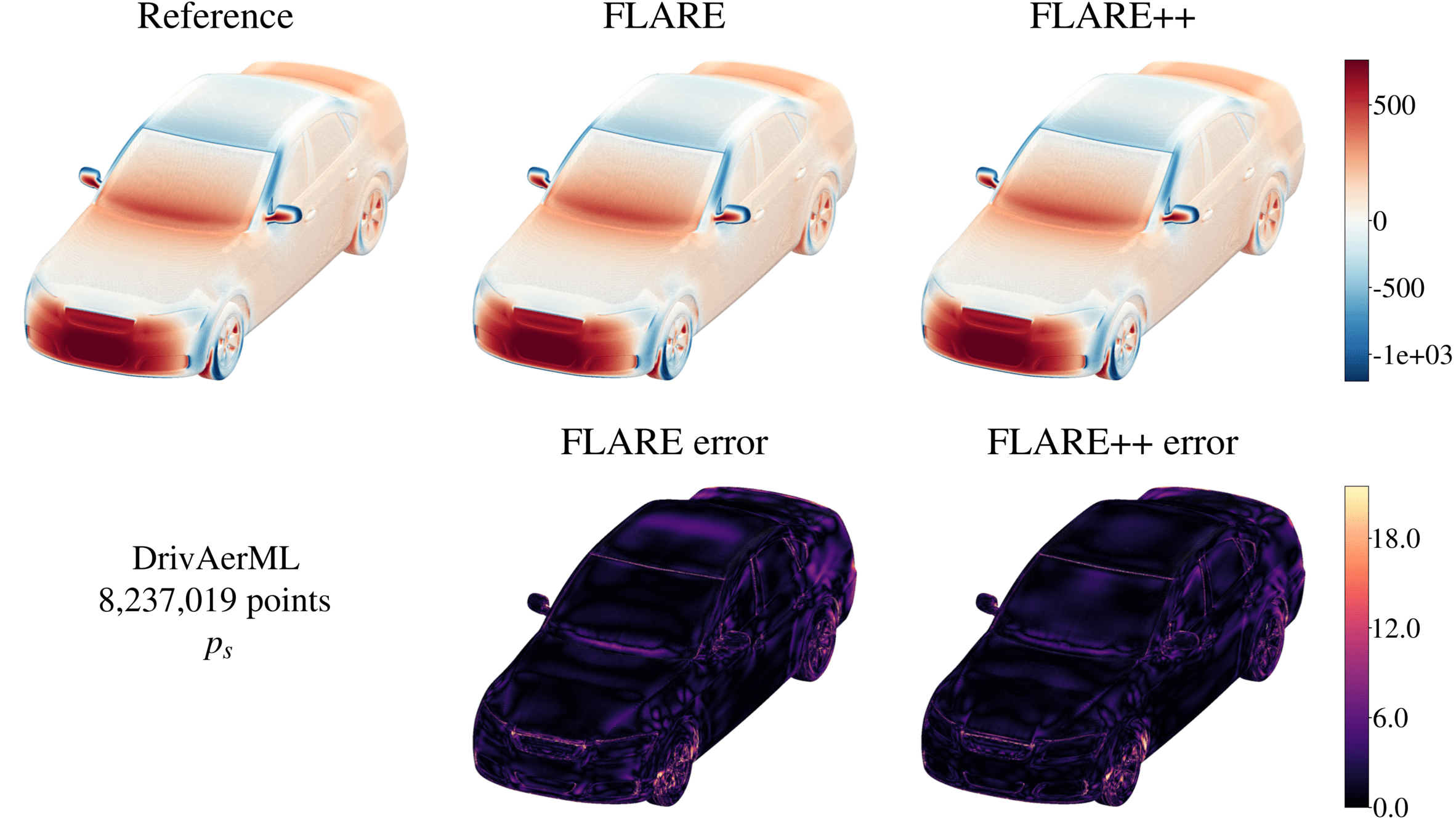
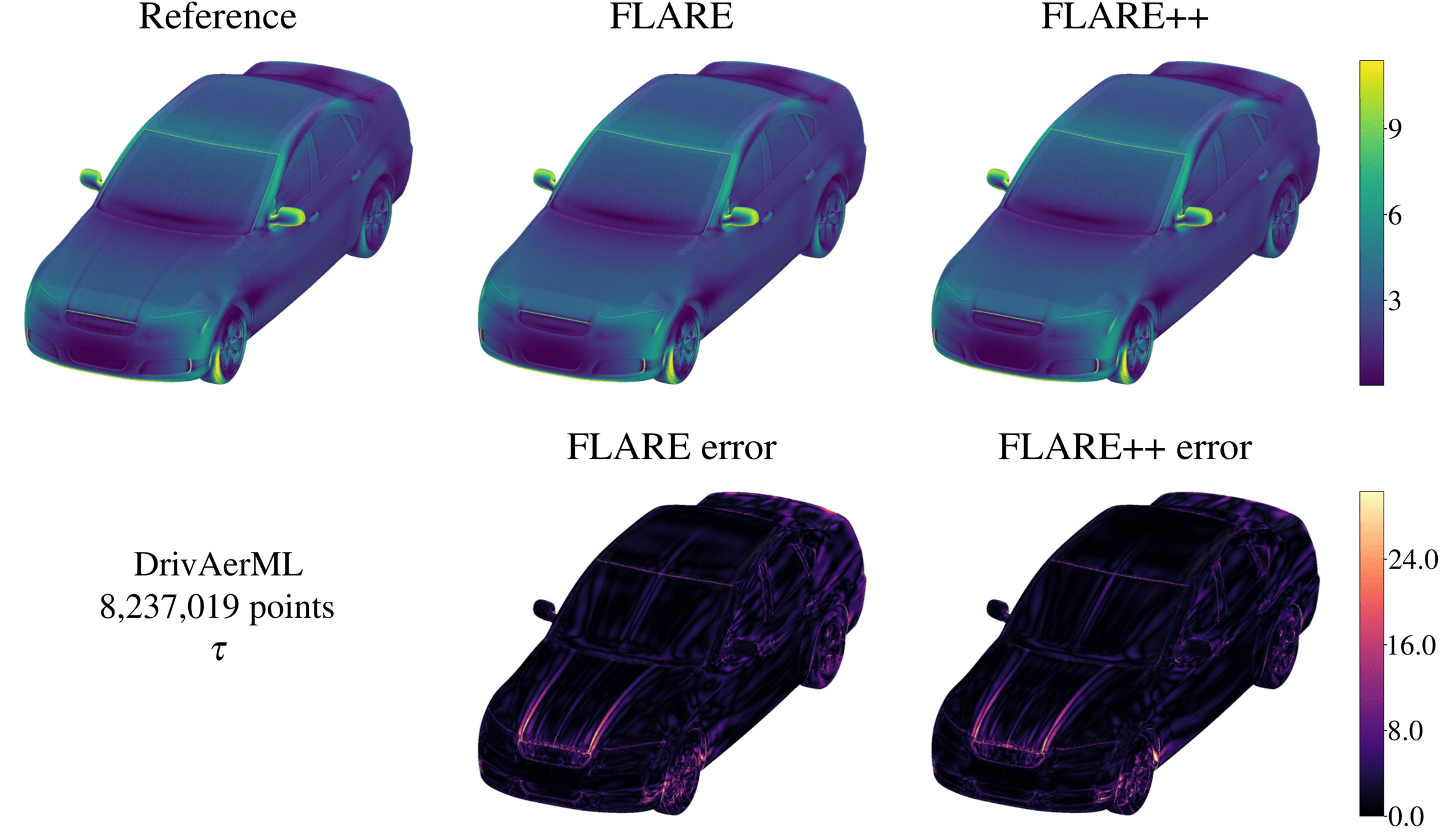
Substantial gains from dynamic routing
Dominant over Transolver family
22
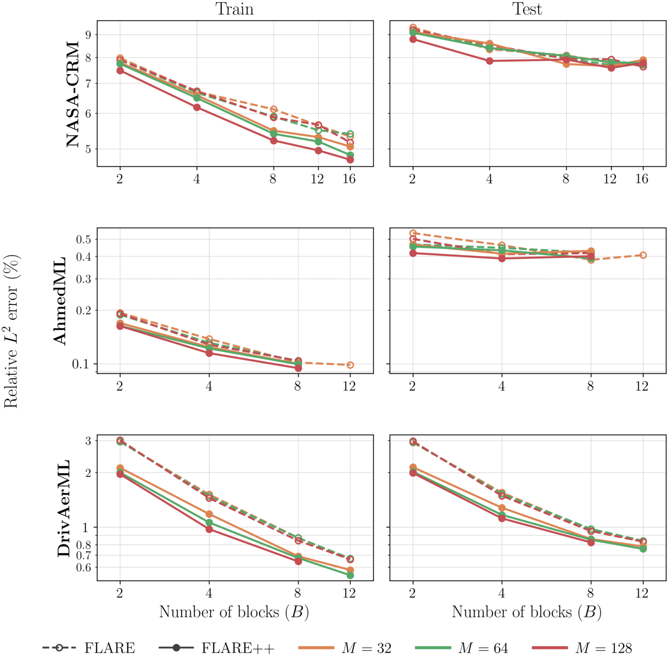
Improved routing substitutes for depth
23
Improved routing substitutes for depth
Continued improvement with \(M\)
24
\(\approx1.2-1.3\times\) slower than FLARE
Inherits FLARE's extreme memory efficiency
25
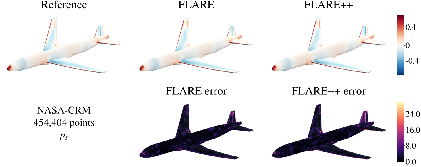
FLARE family is dominant on this problem.
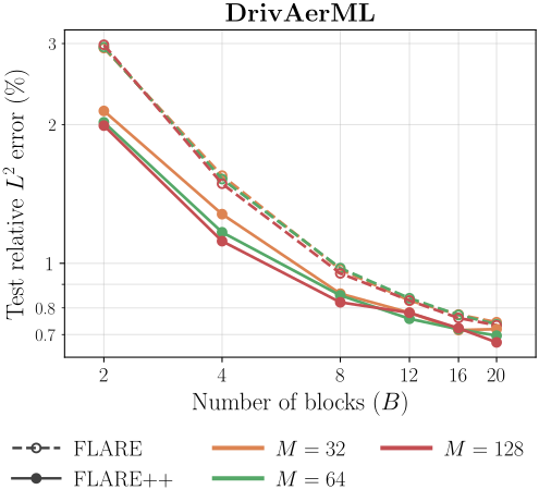
26
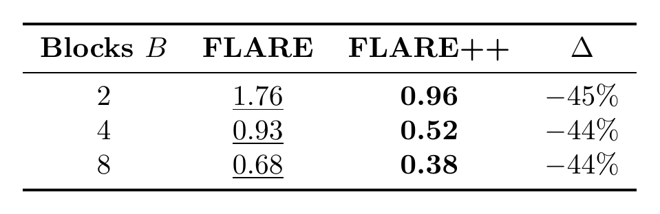
Faster convergence with improved routing
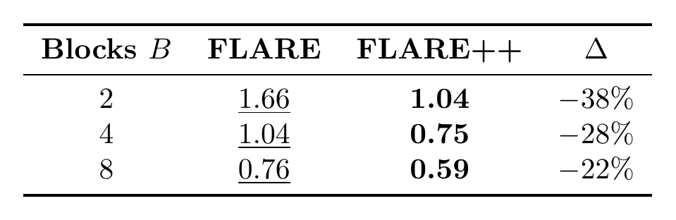
\(\approx30\%\) improvement at \(B=2\)
Continued improvement even at \(B=20\)
27
\(\text{Accuracy (\%)}\)
FLARE++ has highest average accuracy!
28
Future work
Substantial accuracy gains with shorter models
Low-rank attention with dynamic routing
Preprint out on arXiv. Will submit to ICLR
Extend to complex geometries: GeoFLARE++
Consider time-series PDE problems
Demonstrated numerical simulation with neural ansatz
Make attention-based PDE surrogate modeling feasible on large scale meshes
Improve accuracy with smarter compression
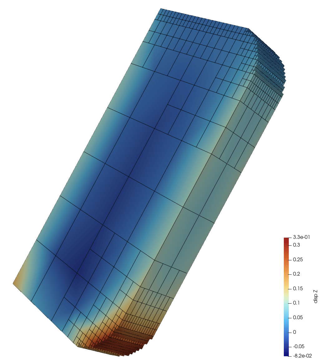
Puri, Vedant, Yongjie Jessica Zhang, and Levent Burak Kara. "FLARE++: Low-rank attention with dynamic token routing." arXiv preprint arXiv:2608.11519 (2026).
Puri, Vedant, Aditya Joglekar, Kevin Ferguson, Yu-hsuan Chen, Yongjie Jessica Zhang, and Levent Burak Kara. "FLARE: Fast Low-rank Attention Routing Engine." arXiv preprint arXiv:2508.12594 (2025).
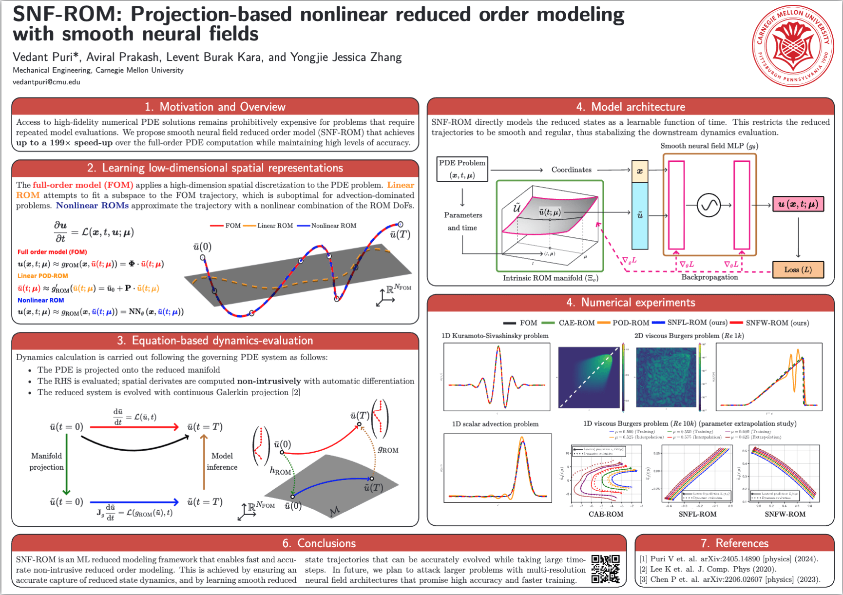
Puri, Vedant, Aviral Prakash, Levent Burak Kara, and Yongjie Jessica Zhang. "SNF-ROM: Projection-based nonlinear reduced order modeling with smooth neural fields." Journal of Computational Physics 532 (2025): 113957.
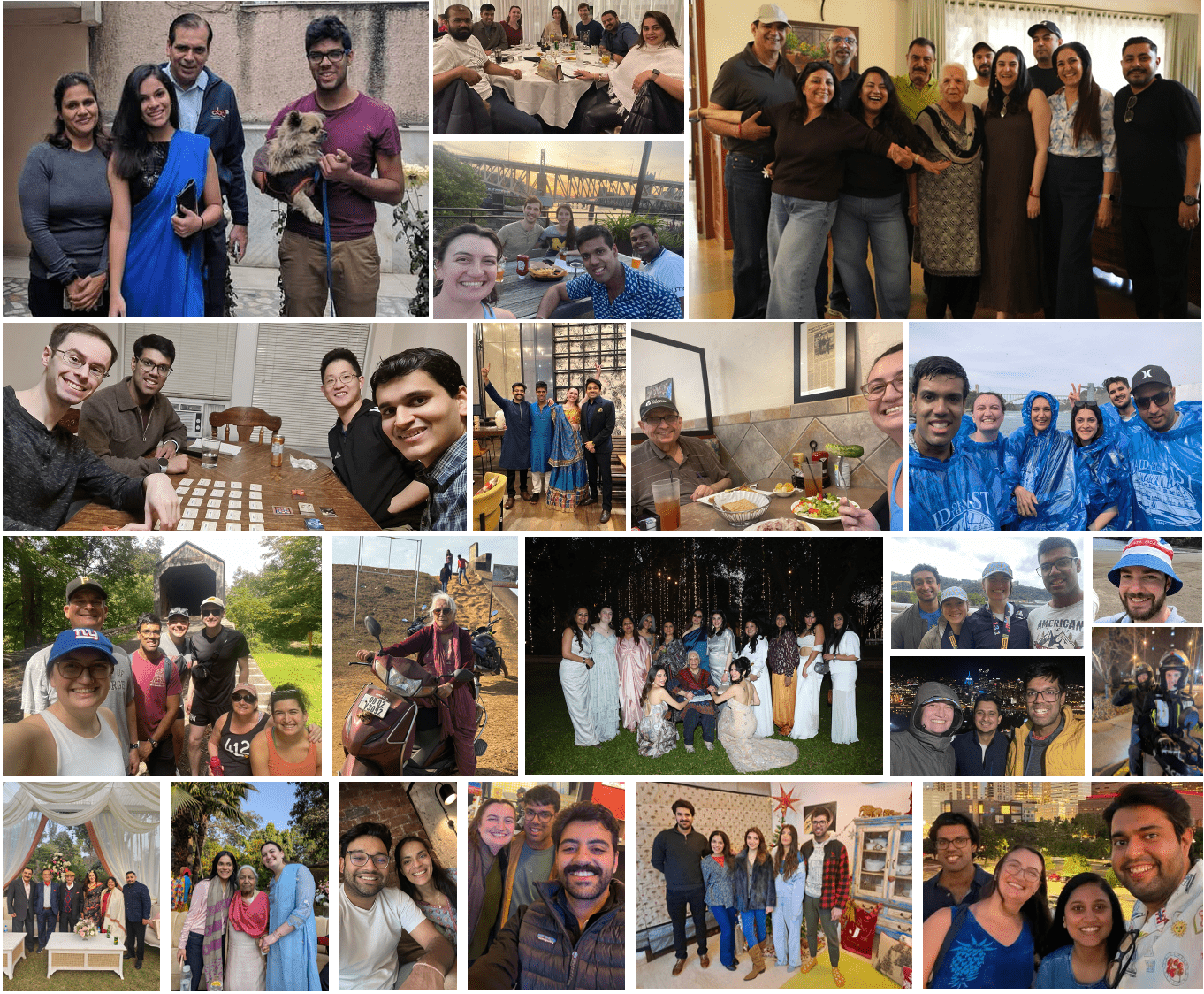
Thank you to CBML, VDEL for support and guidance over the years.
Dr. Levent Burak Kara
Dr. Yonjie Jessica Zhang
Dr. Amir Barati Farimani
Dr. Krishna Garikipati
Dr. Varun Shankar
Dr. Ramesh Balakrishnan
Dr. Romit Maulik
Dr. Venkatsubramanium Viswanathan
Dr. Aviral Prakash
Dr. Aditya Joglekar
Dr. Kevin Ferguson
Dr. Y-hsuan Chen
Sri Datta Ganesh Bandreddi
7
Full order model (FOM)
7
Full order model (FOM)
Linear POD-ROM
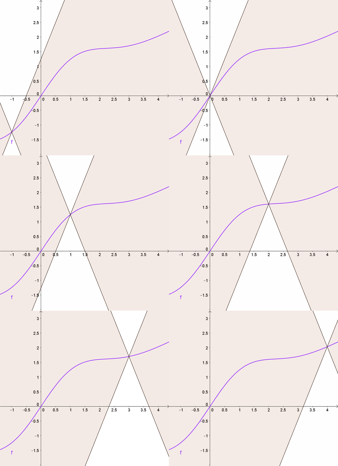
Large Kolmogorov \(N\)-width
in advection problems
7
Full order model (FOM)
Linear POD-ROM
Nonlinear ROM
\({u}(x)=\)
Large Kolmogorov \(N\)-width
in advection problems
6
Learn low-dimensional solution representation with data + evolve with physics.
High-dimensional simulation data
Collect and compress data
Evolve ODE on low-dim manifold
Cost savings from solving smaller ODE system.
Large Kolmogorov \(N\)-width in advection problems
7
[1] Lee & Carlberg — Nonlinear manifold ROM via CNN autoencoders (JCP 2020)
\(\text{Encoder}\)
\(\text{Decoder}\)
Deviation in latent physics solve
2D Burgers \(\mathit{Re}=1\mathit{k}\)
Grid-dependent inference-cost
Not amenable to hyper-reduction
8
Change the solution representation to coordinate neural fields.
\(\text{PDE Problem}\)
\((\boldsymbol{x}, t, \boldsymbol{\mu})\)
\(\text{Coordinates}\)
\(\text{Neural field MLP }(g_\theta)\)
\(\boldsymbol{x}\)
\(\boldsymbol{u}\left( \boldsymbol{x}, t; \boldsymbol{\mu} \right)\)
\(\text{ Parameters}\)
\( \text{and time}\)
\(\tilde{u}\)
Grid-independent
Supports \(\partial_x\) through autodiff
8
\(\text{Loss } (L)\)
\(\text{Backpropagation}\)
\(\nabla_\theta L\)
\(\nabla_\varrho L\)
\(\nabla_\theta L\)
Change the solution representation to coordinate neural fields.
\(\tilde{u}\)
\(\text{PDE Problem}\)
\((\boldsymbol{x}, t, \boldsymbol{\mu})\)
\(\text{ Parameters}\)
\( \text{and time}\)
\(\text{ Intrinsic ROM manifold}\)
\(\text{Coordinates}\)
\(\text{Neural field MLP }(g_\theta)\)
\(\boldsymbol{x}\)
\(\boldsymbol{u}\left( \boldsymbol{x}, t; \boldsymbol{\mu} \right)\)
Grid-independent
Supports \(\partial_x\) through autodiff
Direct control over the complexity of latent trajecories
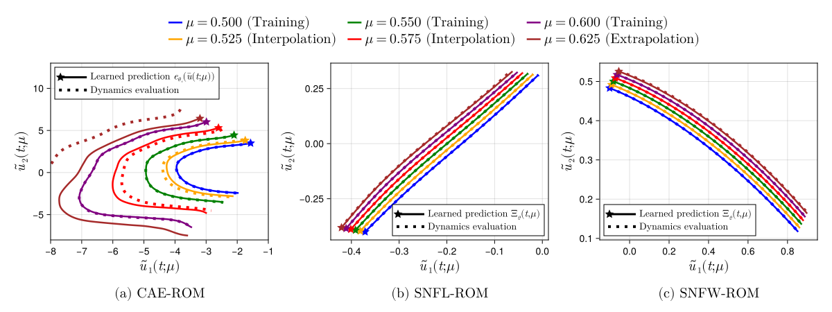
11
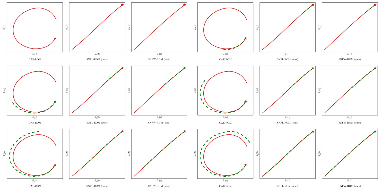
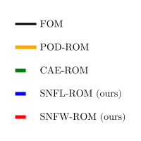
\(\text{CAE-ROM}\) [1]
\(\text{SNFL-ROM (ours)}\)
\(\text{SNFW-ROM (ours)}\)
Online dynamics solve matches learned trajectories
Online evaluation deviates!
Distribution of reduced states \((\tilde{u})\)
[1] Lee & Carlberg — Nonlinear manifold ROM via CNN autoencoders (JCP 2020)
9
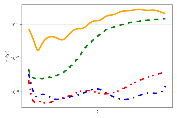
\(\text{CAE-ROM}\) [1]
\(\text{SNFL-ROM (ours)}\)
\(\text{SNFW-ROM (ours)}\)
Relative error
[1] Lee & Carlberg — Nonlinear manifold ROM via CNN autoencoders (JCP 2020)
\([1]\)
\(\text{DoFs: }500\text{k} \to 2\)
\(\text{Time }(t)\)
\(\text{Relative Error}(t)\)
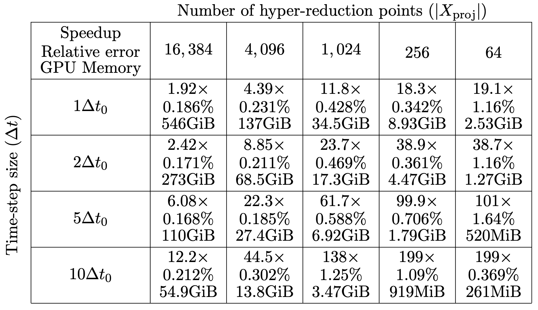
\(199\times\) speed-up
9
Supervised learning problem jointly learns latent trajectories and data manifold.
\(\text{Loss } (L)\)
\(\text{Backpropagation}\)
\(\nabla_\theta L\)
\(\nabla_\varrho L\)
\(\nabla_\theta L\)
\(\text{PDE Problem}\)
\((\boldsymbol{x}, t, \boldsymbol{\mu})\)
\(\text{ Parameters}\)
\( \text{and time}\)
\(\text{ Intrinsic ROM manifold}\)
\(\text{Coordinates}\)
\(\text{Smooth neural field MLP }(g_\theta)\)
\(\tilde{u}\)
\(\boldsymbol{x}\)
\(\boldsymbol{u}\left( \boldsymbol{x}, t; \boldsymbol{\mu} \right)\)
Force \( t \mapsto \tilde{u}(t) \) to be simple, e.g., shallow MLP.
Coordinate MLPs with sinusoidal activations offers grid-independence.
Replace autoencoder with a direct prediction workflow.
10
SNF-ROM with Lipschitz regularization (SNFL-ROM)
\(\text{Penalize the \textcolor{blue}{Lipschitz constant} of the MLP [arXiv:2202.08345]}\)
\(\text{[enwiki:1230354413]}\)
SNF-ROM with Weight regularization (SNFW-ROM)
\(\text{Directly penalize \textcolor{red}{high-frequency components} in }\dfrac{\text{d}}{\text{d} x}\text{NN}_\theta(x)\)
We present two approaches to learn inherently smooth and accurately differentiable neural field MLPs.
\({x}\)
\({u(x)}\)
High freq. noise
12
SNF-ROM maintains high accuracy even with larger time-steps.
\(\text{Relative error vs time } (\Delta t = \Delta t_0)\)
\(\text{Relative error vs time } (\Delta t = 10\Delta t_0)\)
[1] Lee & Carlberg — Nonlinear manifold ROM via CNN autoencoders (JCP 2020)
13
\(\text{CAE-ROM}\) [1]
\(\text{SNFL-ROM (ours)}\)
\(\text{SNFW-ROM (ours)}\)
\(\text{Relative error }\)
[1] Lee & Carlberg — Nonlinear manifold ROM via CNN autoencoders (JCP 2020)
\([1]\)
17
Over \(20~\text{s}\) per gradient step on a mesh of 1m poins!
[1] Vaswani et al. — “Attention Is All You Need”, NeurIPS 2017
Multiple parallel low-rank pathways
Multi-head cross-attention encoder/decoder
Eliminate latent-space self-attention
Simplify and connect latent attention to low-rank
+Transolver has same nn.Linear(D,M) proj for all heads.
Isolate attention routing as the load-bearing pirmitive
Extreme scalability thanks to SDPA compatibility
16
25
Darcy
Elasticity
Airfoil
FLARE++ improves on FLARE!
Maintains accuracy in FP16
Competitive with full self-attention
11
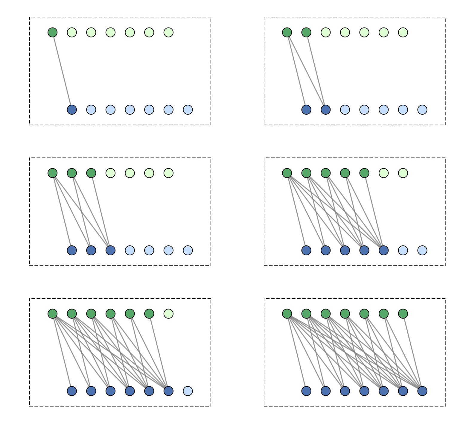
All previous key/value \(\{k_\tau, v_\tau \}_{\tau \leq t}\) must be cached on the GPU.
Major memory and latency bottleneck!
33
[1] Vaswani et al. — “Attention Is All You Need”, NeurIPS 2017
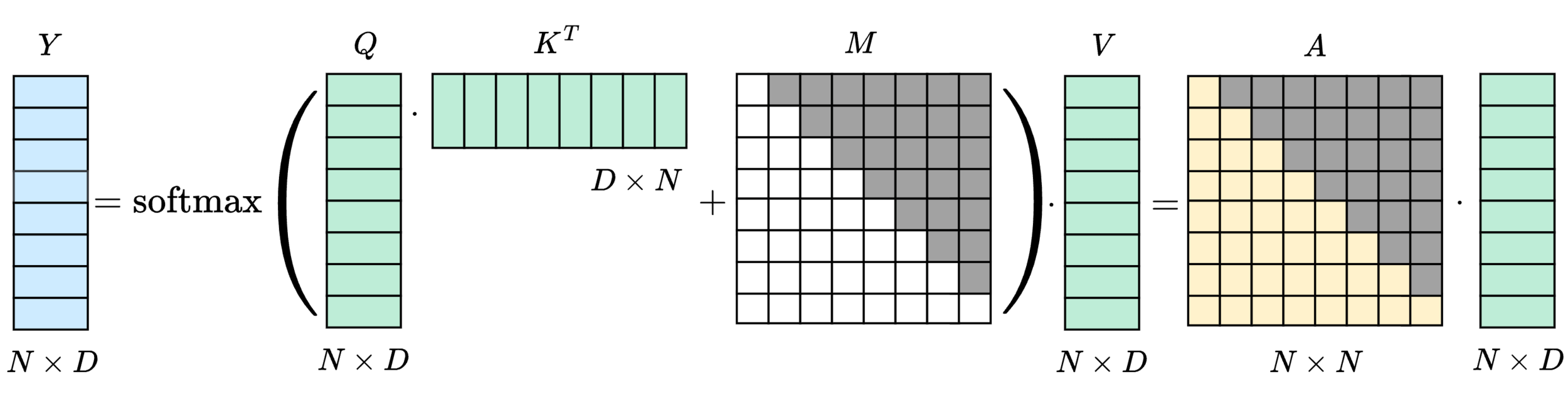
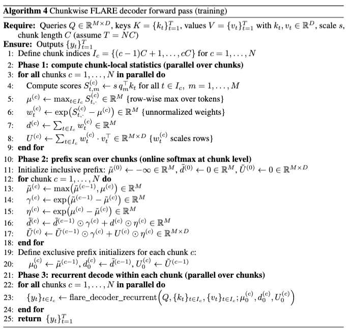
Training algorithm (causal masking)
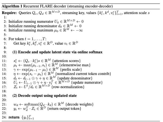
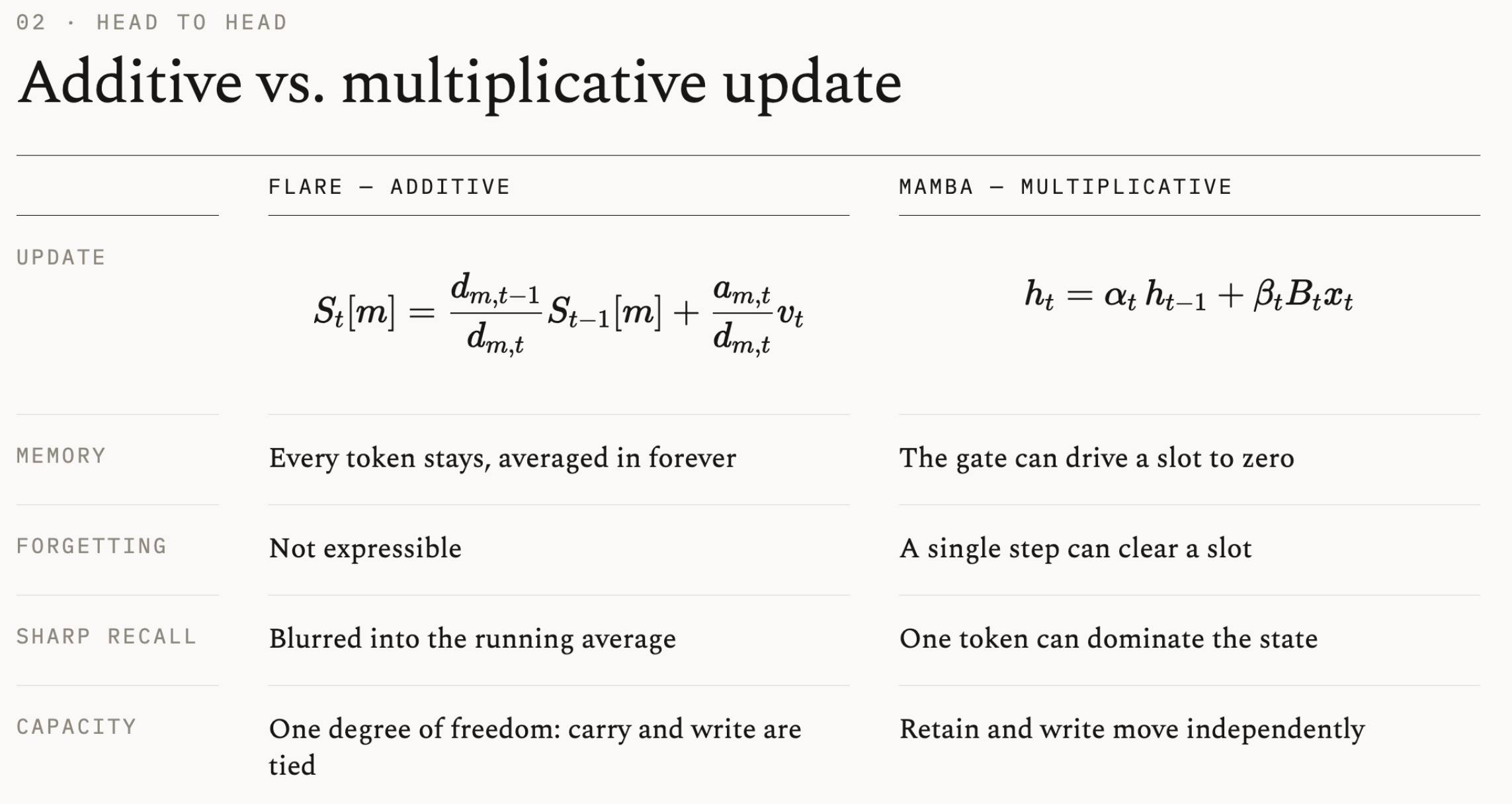
Inference algorithm (recurrence relation)
Dot-products need to be recomputed for every \(q_t\).
\(\mathcal{O}(N^2)\) complexity.
Linear time auto-regressive attention.
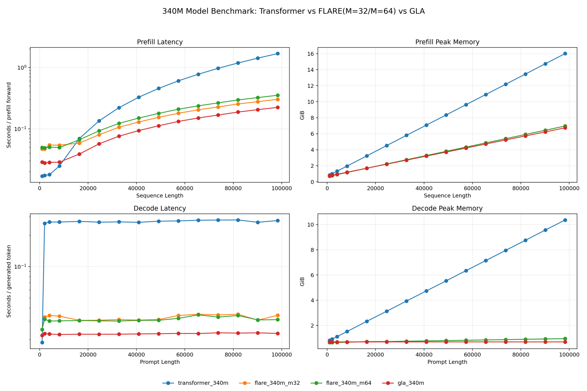
Fixed memory footprint (only store \(\mathcal{O}(M)\) cache).
Flexible latent capacity.
Advantages
Required components
Fused GPU kernels for training and inference.
Bespoke training algorithm for causal FLARE.
Extensive benchmarking and evaluation.
34
Inference algorithm (recurrence rule)
https://github.com/vpuri3/flash-linear-attention-pvt/blob/run/legacy/training/STORYTELLING.md
https://github.com/vpuri3/flash-linear-attention-pvt/blob/run/legacy/training/STORYTELLING.md
https://github.com/vpuri3/flash-linear-attention-pvt/blob/run/legacy/training/STORYTELLING.md
22
22
18
[2] Akhare et al. “High-Fidelity Industrial- Crash Dynamics”, arXiv:2605:27758
[1] Adams et al. “GeoTransolver”, arXiv:2512:20399
[3] Curtosi, et al. "Crash Assessment via Physics-Aware Attention", arxiv:2605:11784
[1]
[2]
FLARE backbone + multiscale geometry feature extractor
[2]
NVIDIA
Norte Dame, GM
SEAT, IDIADA (Spain)
[3]
GeoFLARE architecture
19
[2] Akhare et al. “High-Fidelity Industrial- Crash Dynamics”, arXiv:2605:27758
[1] Adams et al. “GeoTransolver”, arXiv:2512:20399
[3] GitHub:NVIDIA/physicsnemo/examples/structural_mechanics/crash
20
[2] Akhare et al. “High-Fidelity Industrial- Crash Dynamics”, arXiv:2605:27758
[1] Adams et al. “GeoTransolver”, arXiv:2512:20399
[3] GitHub:NVIDIA/physicsnemo/examples/structural_mechanics/crash
By Vedant Puri
Vedant Puri's thesis defense at Carnegie Mellon University