PhD Oral Presentation

Analytical Methods in CS

(and Back!)

Martingales

Privacy

Experts

\int_a^b f(x) \mathrm{d}x

Stochastic Calc.

& Online Learning

Vector Calculus and Probability Theory

Stochastic Calculus

Privacy

Differential Privacy

\displaystyle \mathcal{M}

Output 1

Output 2

Not too far apart

What does it mean for an algorithm \(\mathcal{M}\) to be private?

Differential Privacy: \(\mathcal{M}\) does not rely heavily on any individual

\((\varepsilon, \delta)\)-Diff. Privacy

\(\varepsilon \equiv \) "Privacy leakage", small constant

\(\delta \equiv \) "Chance of failure", usually \(O(1/\text{\#samples})\)

\displaystyle \Bigg \{

Covariance Estimation

\displaystyle x_1, x_2, \dotsc, x_n \sim \mathcal{N}(0, \Sigma)

\displaystyle \Sigma \succ 0

Unknown Covariance Matrix

\displaystyle X \in \mathbb{R}^{d \times n}

\((\varepsilon, \delta)\)-differentially private \(\mathcal{M}\) to estimate \(\Sigma\)

on \(\mathbb{R}^d\)

Goal:

Required even without privacy

Required even for \(d = 1\)

Is this tight?

Exists \((\varepsilon, \delta)\)-DP \(\mathcal{M}\) such that

\displaystyle n = \tilde O\Big(\frac{d^2}{\alpha^2} + \frac{\log(1/\delta)}{\varepsilon} + \frac{d^2}{\alpha \varepsilon}\Big)

\displaystyle \mathbb{E}[\lVert\mathcal{M}(X) - \Sigma\rVert_F^2] \leq \alpha^2

samples

Known algorithmic results

with

Our Results - New Lower Bounds

Theorem

For any \((\varepsilon, \delta)\)-DP algorithm \(\mathcal{M}\) such that

\displaystyle \mathbb{E}\big[\lVert\mathcal{M}(X) - \Sigma\rVert_F^2\big] \leq \alpha^2 = O(d)

and

\displaystyle \delta = O\Big( \frac{1}{n \ln n}\Big)

we have

\displaystyle n = \Omega\Big(\frac{d^2}{\alpha\varepsilon}\Big)

Our results generalize both of them

Nearly highest reasonable value

\displaystyle \delta = \tilde O\Big(\frac{1}{d^2}\Big) = o\Big(\frac{1}{n}\Big)

\displaystyle \alpha = O(1)

[Kamath et al. 22]

Previous lower bounds required

\displaystyle n = \Omega\big(\tfrac{d^2}{\alpha\varepsilon}\big)

\displaystyle \Bigg \{

[Narayanan 23]

OR

Lower Bounds via Fingerprinting

A measure of the correlation between \(z\) and \(\mathcal{M}(X)\)

Correlation statistic

\displaystyle \mathcal{A}(z, \mathcal{M}(X))

\displaystyle \mathbb{E}[|\mathcal{A}(z, \mathcal{M}(X))|]

If \(z \sim \mathcal{N}(0, \Sigma)\) indep. of \(X\)

small

\displaystyle \mathbb{E}[\mathcal{A}(x_i, \mathcal{M}(X))]

If \(\mathcal{M}\) is accurate

large

Fingerprinting Lemma

\displaystyle \Sigma

\displaystyle zz^{\intercal}

\displaystyle \mathcal{M}(X)

\displaystyle \Sigma

\displaystyle x_3 x_3^{\intercal}

\displaystyle x_1 x_1^{\intercal}

\displaystyle x_2 x_2^{\intercal}

\displaystyle x_4 x_4^{\intercal}

\displaystyle \mathcal{M}(X)

Approx. equal by privacy

Score Statistic

\displaystyle \mathcal{A}(z, \mathcal{M}(X)) = \big\langle\mathcal{M}(X) - \Sigma, \nabla_{\Sigma} \log p_{\mathcal{N}}(z \;|\; \Sigma)\big\rangle

Score function

Score Attack Statistic

To get a fingerprinting lemma, we need to randomize \(\Sigma\) so that

\displaystyle \mathbb{E}[\mathcal{A}(x_i, \mathcal{M}(X))]

is large

Previous work

\(\Sigma\) with "small radius" \(\implies\) Weak FP Lemma

\(\Sigma\) with "large radius" \(\implies\) hard to bound \(\mathbb{E}[|\mathcal{A}(z, \mathcal{M}(X))|]\)

\displaystyle \mathcal{A}(z, \mathcal{M}(X)) = \langle\mathcal{M}(X) - \Sigma, z z^{\intercal} - \Sigma \rangle

\displaystyle zz^{\intercal}

\displaystyle \mathcal{M}(X)

\displaystyle \Sigma

New Fingerprinting Lemma

Fingerprinting Lemma

Need to Lower Bound

\displaystyle \mathbb{E}\Big[ \sum_{i,j }\partial_{ij} \; g(\Sigma)_{ij}\Big]

\displaystyle g(\Sigma) = \mathbb{E}[\mathcal{M}(X)]

\(\Sigma \sim\) Wishart leads to elegant analysis

Stein-Haff Identity

"Move the derivative" from \(g\) to \(p\) with integration by parts

\displaystyle \mathrm{div} g(\Sigma)

\displaystyle \mathbb{E}[ \mathrm{div} g(\Sigma)] = \int \mathrm{div} g(\Sigma) \cdot p(\Sigma) \mathrm{d}\Sigma

Stokes' Theorem

\displaystyle \sum_{i = 1}^n \mathbb{E}[\mathcal{A}(x_i, \mathcal{M}(X))]

\displaystyle \geq \Omega(d^2)

\displaystyle O(n \alpha \varepsilon) \geq

FP Lemma

Upper Bound

Experts

Player

Adversary

\(n\) Experts

0.5

0.1

0.3

0.1

Probabilities

p_t

1

-1

0.5

-0.3

Gains

g_t \in [-1,1]^n

Player's gain:

\langle g_t, p_t \rangle

\mathbb{E}[g_t(i)]

Prediction with Expert's Advice

\displaystyle \mathrm{Regret}(T) = \max_{i = 1, \dotsc, n} \sum_{t = 1}^T g_t(i) - \sum_{t = 1}^T \langle g_t, p_t \rangle

Gain of Best Expert

Player's Gain

Quantile Regret

Best Expert

Best Experts

\(\varepsilon\)-fraction

\displaystyle \Bigg \}

Multiplicative Weights Update:

\displaystyle \lesssim \sqrt{T \ln (1/\varepsilon)}

Needs knowledge of \(\varepsilon\)

We design an algorith with \(\sqrt{T \ln(1/\varepsilon)}\) quantile regret

for all \(\varepsilon\) and best known leading constant

\displaystyle \sum_{t = 1}^T g_t(i_{\varepsilon}) - \sum_{t = 1}^T \langle g_t, p_t \rangle

Gain of

top \(\varepsilon n \) expert

\(\varepsilon\)-Quantile Regret

Moving to Continuous Time

Analysis often becomes clean

Sandbox for design of optimization algorithms

Key Question: How to model non-smooth (online) optimization in continuous time?

Why go to ?

continuous time

Discrete Time

\displaystyle G_t(i) = \sum_{s = 1}^t g_s(i)

Useful perspective: \(G(i)\) is a realization of a random walk

Continuous Time

\(G_t(i)\) is a realization of a Brownian Motion

\displaystyle G_t(i) = B_t(i)

Worst-case =

Probability 1

Improved Quantile Regret

Potential based players

\displaystyle p(t) \propto \nabla \Phi(t, R(t))

Stochastic Calculus suggests \(\Phi\) that satisfy the Backwards Heat Equation

\;\;\;\;\Phi + \;\;\;\;\;\;\; \Phi = 0

\displaystyle \partial_t

\displaystyle \tfrac{1}{2}\partial_{xx}

\displaystyle \mathrm{QuantRegret}(T, \varepsilon) \leq 2\sqrt{2 T \ln(1/\varepsilon)} + 6 \sqrt{T}

For all \(\varepsilon\)

Using this potential*, we get

Best leading constant

Discrete time analysis is IDENTICAL to continuous time analysis

*(with a slightly bigger cnst. in the BHE)

Anytime Experts

Question:

Are the minimax regret with and without knowledge of \(T\) different?

fixed-time

anytime

fixed-time

\displaystyle \sqrt{2 T \ln n}

Theorem: In Continuous Time, both are equal if Brownian Motions are independent.

MinmaxRegret

\displaystyle 2\sqrt{T \ln n}

\displaystyle \leq

Can we get better lower bounds?

=

?

Martingales

Motivation: Expected Regret

\displaystyle \mathrm{Regret}(\tau) = \lVert \phantom{G_\tau} \rVert_{\infty} - \phantom{A_\tau}

\displaystyle G_\tau

\displaystyle A_\tau

Player's Total Gain

Vector of the Experts' Gains

\displaystyle \mathbb{E}[A_\tau] = 0

High expected regret \(\implies\) anytime lower bound

Max expected anytime regret without independent experts?

Anytime Regret \(\equiv\) \(\tau\) is a stopping time

\displaystyle \frac{\mathbb{E}[\mathrm{Regret}(\tau)]}{\mathbb{E}[\sqrt{\tau}]}

How big can

be?

Norm of High-Dimensional Martingales

For a martingale \((G_t)_{t \geq 0}\), find upper and lower bounds to

\displaystyle \frac{\mathbb{E}[\lVert G_{\tau}\rVert_{\infty}]}{\mathbb{E}[\sqrt{\tau}]}

sup

\displaystyle \Bigg\{

\displaystyle :

\displaystyle \tau

is a stopping time

\displaystyle \Bigg\}

\displaystyle K_n =

\displaystyle K_n

\displaystyle \leq \lambda(n-1)

\displaystyle c_n \leq

\displaystyle \sim \sqrt{2 \ln n}

\displaystyle \sqrt{2 \ln n} \sim

No assumptions

on the dependency between coordinates

Theorem

If \(G_t(i)\) is a Brownian motion for all \(i = 1, \dotsc, n\), then

Evidence that Anytime Lower Bounds for

continuous experts needs new techniques

Other Results

For a martingale \((G_t)_{t \geq 0}\), find upper and lower bounds to

\displaystyle \frac{\mathbb{E}[\lVert G_{\tau}\rVert_{\infty}]}{\mathbb{E}[\sqrt{\tau}]}

sup

\displaystyle \Bigg\{

\displaystyle :

\displaystyle \tau

is a stopping time

\displaystyle \Bigg\}

\displaystyle K_n =

Similar upper bounds when \(G_t(i)\) has smooth quadratic variation

If \(G_t(i)\) is a discrete martingale with increments in \([-1,1]\), we have

\displaystyle K_n\leq \lambda(n-1)

Beyond Brownian Motion

Discrete Martingales

Discrete Ito's Lemma

Main Ideas of the Analysis

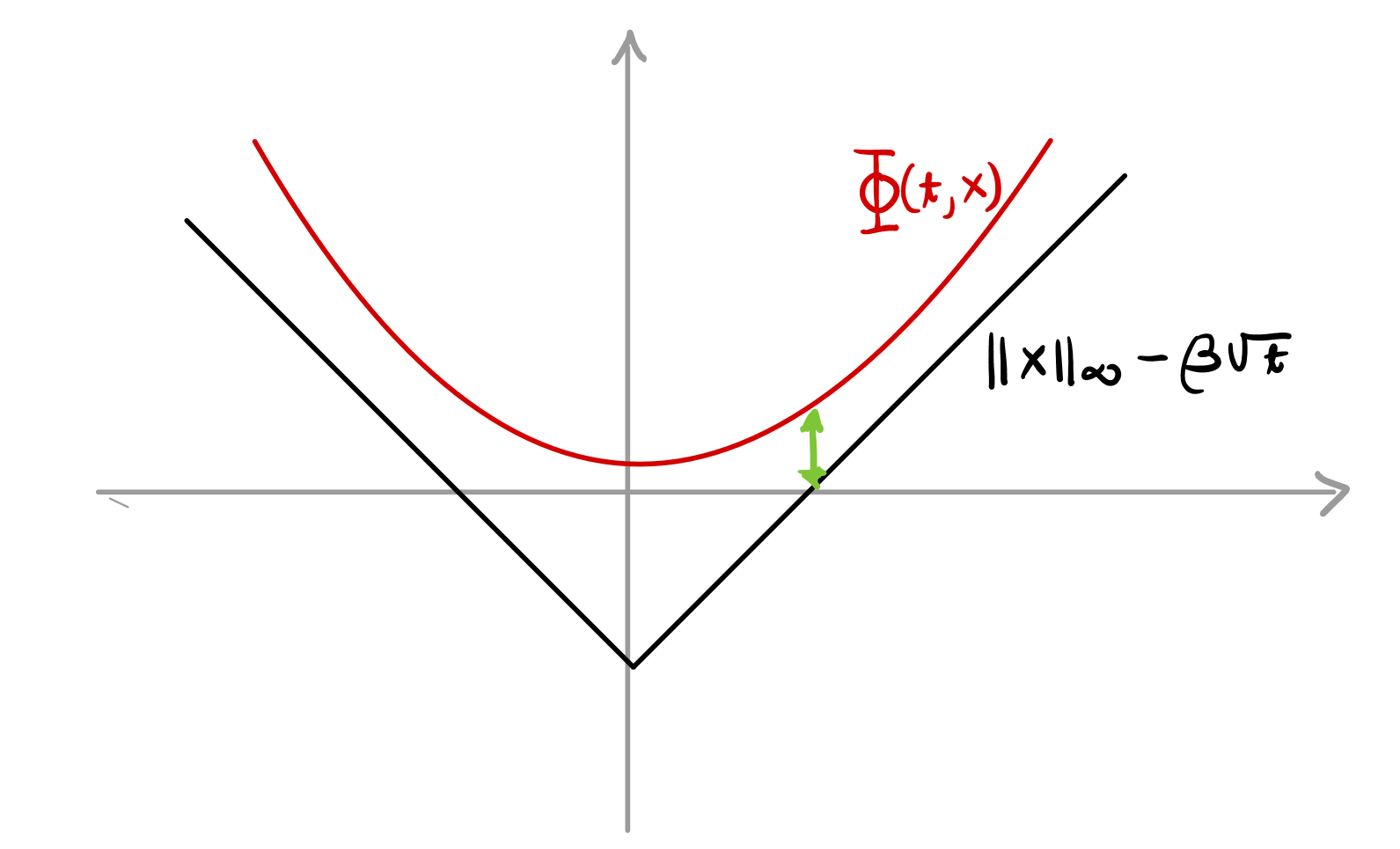
Goal:

\displaystyle \mathbb{E}\big[\lVert G_\tau \rVert_{\infty} - \beta \sqrt{\tau} \big] \leq 0

\displaystyle = \mathbb{E}\big[\lVert G_{0} \rVert - \beta \sqrt{0} \big]

non-smooth \(\implies\) hard to show it is a supermartingale

Idea:

Design a smooth function \(\Phi\) such that

\((\Phi(t, G_t))_{t \geq 0}\)

is a supermartingale

and

\displaystyle \lVert x \rVert_{\infty} - \beta \sqrt{t} \leq \Phi(t, x)

Backwards Heat Eq.

Tune Constants

Fingerprinting and Stein's Identity

\displaystyle \mathcal{A}(z, \mathcal{M}(X)) = \big\langle\mathcal{M}(X) - \Sigma, \nabla_{\Sigma} \log p_{\mathcal{N}}(z \;|\; \Sigma)\big\rangle

Score function

If \(z \sim \mathcal{N}(0, \Sigma)\) indep. of \(X\)

For \(x_1, \dotsc, x_n\) from \(X\)

\displaystyle \mathbb{E}[|\mathcal{A}(z, \mathcal{M}(X))|] \leq \frac{\alpha}{\lambda_{\min}(\Sigma)}

\displaystyle \sum_{i = 1}^n \mathbb{E}[\mathcal{A}(x_i, \mathcal{M}(X))] = \sum_{i,j} \frac{\partial}{\partial_{\Sigma_{ij}}} \mathbb{E}[\mathcal{M}(X)_{ij}]

\(= \Theta(d^2)\) if \(\mathbb{E}[\mathcal{M(X)}] = \Sigma\)

Modeling Adversarial Costs in Continuous Time

Total gains of expert \(i\):

\displaystyle G_t(i) = \sum_{s = 1}^t g_s(i)

Useful perspective: \(G(i)\) is a realization of a random walk

realization of a Brownian Motion

Probability 1 = Worst-case

Discrete Time

Continuous Time

\displaystyle G_t(i) = B_t(i)

Score Statistic

\displaystyle \mathcal{A}(z, \mathcal{M}(X)) = \big\langle\mathcal{M}(X) - \Sigma, \nabla_{\Sigma} \log p_{\mathcal{N}}(z \;|\; \Sigma)\big\rangle

Main Property

Score function

Score Attack Statistic

Previous work:

\displaystyle \mathcal{A}(z, \mathcal{M}(X)) = \langle\mathcal{M}(X) - \Sigma, z z^{\intercal} - \Sigma \rangle

\displaystyle \sum_{i = 1}^n \mathbb{E}[\mathcal{A}(x_i, \mathcal{M}(X))] = \sum_{i,j} \phantom{\frac{\partial}{\partial_{\Sigma_{ij}}}} \mathbb{E}[\mathcal{M}(X)_{ij}]

\displaystyle \frac{\partial}{\partial_{\Sigma_{ij}}}

Want random \(\Sigma\) such that this is large in expectation

Covariance Estimation

\displaystyle x_1, x_2, \dotsc, x_n \sim \mathcal{N}(0, \Sigma)

\displaystyle X \in \mathbb{R}^{d \times n}

Known bounds on sample complexity

There is an \((\varepsilon, \delta)\)-DP mechanism \(\mathcal{M}\) such that

\displaystyle n = \tilde O\Big(\frac{d^2}{\alpha^2} + \frac{\log(1/\delta)}{\varepsilon} + \frac{d^2}{\alpha \varepsilon}\Big)

\displaystyle \Sigma \succ 0

Unknown Covarince Matrix

on \(\mathbb{R}^d\)

\displaystyle \mathbb{E}[\lVert\mathcal{M}(X) - \Sigma\rVert_F^2] \leq \alpha^2

for some

Required even without privacy

Required even for \(d = 1\)

Is this tight?

Lower Bounds via Fingerprinting

Correlation statistic

\displaystyle \mathcal{A}(z, \mathcal{M}(X)) = \langle\mathcal{M}(X) - \Sigma, z z^{\intercal} - \Sigma \rangle

\displaystyle \mathbb{E}[|\mathcal{A}(z, \mathcal{M}(X))|]

If \(z \sim \mathcal{N}(0, \Sigma)\) indep. of \(X\)

small

\displaystyle \mathbb{E}[\mathcal{A}(x_i, \mathcal{M}(X))]

If \(\mathcal{M}\) is accurate

large

\displaystyle \mathcal{M}(X)

\displaystyle zz^{\intercal}

\displaystyle \Sigma

\displaystyle zz^{\intercal}

\displaystyle \mathcal{M}(X)

\displaystyle x_1 x_1^{\intercal}

\displaystyle \Sigma

\displaystyle x_3 x_3^{\intercal}

\displaystyle x_2 x_2^{\intercal}

\displaystyle x_4 x_4^{\intercal}

Approx. equal by privacy

Fingerprinting Lemma

for covariance estimation

\(\mathcal{A}(z, \mathcal{M}(X))\)

leads to limited lower bounds

Lower Bounds via Fingerprinting

Correlation statistic

\displaystyle \mathcal{A}(z, \mathcal{M}(X)) = \langle\mathcal{M}(X) - \Sigma, z z^{\intercal} - \Sigma \rangle

\displaystyle \mathbb{E}[|\mathcal{A}(z, \mathcal{M}(X))|]

If \(z \sim \mathcal{N}(0, \Sigma)\) indep. of \(X\)

small

\displaystyle \mathbb{E}[\mathcal{A}(x_i, \mathcal{M}(X))]

If \(\mathcal{M}\) is accurate

large

\displaystyle \mathcal{M}(X)

\displaystyle zz^{\intercal}

\displaystyle \Sigma

\displaystyle zz^{\intercal}

\displaystyle \mathcal{M}(X)

\displaystyle x_1 x_1^{\intercal}

\displaystyle \Sigma

\displaystyle x_3 x_3^{\intercal}

\displaystyle x_2 x_2^{\intercal}

\displaystyle x_4 x_4^{\intercal}

Approx. equal by privacy

Fingerprinting Lemma

for covariance estimation

\(\mathcal{A}(z, \mathcal{M}(X))\)

leads to limited lower bounds

Online Learning and Experts

Prediction with Expert's Advice

Player

Adversary

\(n\) Experts

0.5

0.1

0.3

0.1

Probabilities

x_t

1

-1

0.5

-0.3

Costs

\ell_t

Player's loss:

\langle \ell_t, x_t \rangle

Adversary knows the strategy of the player

\mathbb{E}[\ell_t(i)]

Performance Measure - Regret

\displaystyle \mathrm{Regret}(T) = \sum_{t = 1}^T \langle \ell_t, p_t \rangle - \min_{i = 1, \dotsc, n} \sum_{t = 1}^T \ell_t(i)

Loss of Best Expert

Player's Loss

\displaystyle \mathrm{Regret}(T) \leq \sqrt{2 T \ln n}

Optimal!

\displaystyle \mathbb{E}[\mathrm{Regret}(T)] \geq \sqrt{2 T \ln n}(1 - o(1))

For random \(\pm 1\) costs

Multiplicative Weights Update:

\displaystyle p_{t+1}(i) \propto p_t(i) \cdot \exp(-\eta \ell_t(i) )

(Hedge)

Why Learning with Experts?

Boosting in ML

Understanding sequential prediction

Universal Optimization

Solving SDPs, TCS, Learning theory...

Motivating Problem - Fixed Time vs Anytime

MWU regret

\displaystyle \mathrm{Regret}(T) \leq \sqrt{2 T \ln n}

when \(T\) is known

\displaystyle \mathrm{Regret}(T) \leq 2\sqrt{T \ln n}

when \(T\) is not known

\displaystyle \Bigg\{

anytime

fixed-time

Does knowing \(T\) gives the player an advantage?

[Harvey, Liaw, Perkins, Randhawa '23]

Random cost are (probably) too easy to show separation

[VSP, Liaw, Harvey '22]

Anytime > Fixed time for 2 experts + optimal algorithm

+ new algorithms for quantile regret!

With stochastic calculus:

Continuous Experts' Problem

Modeling Adversarial Costs in Continuous Time

Analysis often becomes clean

Sandbox for design of optimization algorithms

Gradient flow is useful for smooth optimization

\displaystyle \partial_t x_t = - \nabla f(x_t)

How to model non-smooth (adversarial) optimization in continuous time?

Why go to ?

continuous time

Modeling Adversarial Costs in Continuous Time

Total loss of expert \(i\):

\displaystyle L_t(i) = \sum_{s = 1}^t \ell_s(i)

Useful perspective: \(L(i)\) is a realization of a random walk

realization of a Brownian Motion

Probability 1 = Worst-case

Discrete Time

Continuous Time

\displaystyle L_t(i) = B_t(i)

The Continuous Time Model

Discrete time

Continuous time

\displaystyle \mathrm{Regret}(t) = \max_{i} R_t(i)

\displaystyle R_t(i) = A_t - L_t(i)

\displaystyle L_t(i) =B_t(i)

\displaystyle L_t(i) = \mathrm{Rand. Walk}

Cummulative loss

Player's cummulative loss

\displaystyle \sum_{t = 1}^T\langle p_t, \Delta L_t\rangle

\displaystyle \int_0^T\langle p_t, \mathrm{d} L_t \rangle

\displaystyle A_t

Player's loss per round

\displaystyle \langle p_t, \ell_t\rangle

\displaystyle \langle p_t, \mathrm{d} L_t \rangle

[Freund '09]

\displaystyle \Delta L_t

MWU in Continuous Time

Potential based players

\displaystyle p(t) \propto \nabla_x \Phi(t, R_t)

\displaystyle \Phi(t, R(t)) = \ln \left( \sum_{i} e^{-\eta_t R_t(i)} \right)

\displaystyle p_t(i) \propto e^{-\eta_t L_t(i)}

\displaystyle \implies

Regret bounds

\displaystyle \mathrm{Regret}(T) \leq \sqrt{2 T \ln n}

when \(T\) is known

\displaystyle \mathrm{Regret}(T) \leq 2\sqrt{T \ln n}

when \(T\) is not known

anytime

fixed-time

\displaystyle \Bigg\{

MWU!

Same as discrete time!

Idea: Use stochastic calculus to guide the algorithm design

with prob. 1

A Peek Into the Analysis

Ito's Lemma

(Fundamental Theorem of Stochastic Calculus)

\displaystyle \Phi(T, R_T) - \Phi(0, R_0)

\displaystyle + \int_0^T \Big( \partial_t \Phi(t, R_t) + \frac{1}{2}\partial_{xx} \Phi(t, R_t) \Big) \mathrm{d} t

\displaystyle = \int_0^T \nabla_x \Phi(t, R_t) \mathrm{d} R_t

\displaystyle f(B_t) - f(B_0) = \int_{0}^T f'(B_t) \mathrm{d} B_t

\displaystyle + ~\frac{1}{2} \int_{0}^T f'' (B_t) \mathrm{d} t

\(B_t\) is very non-smooth \(\implies\) second-order terms matter

\(n = 1\)

Ito's Lemma

Potential does not change too much

\displaystyle = 0

\displaystyle \approx 0

Would be great

A Peek Into the Analysis

Potential based players

\displaystyle p(t) \propto \nabla \Phi(t, R(t))

\displaystyle \mathrm{Regret}(T) \leq \sqrt{2 T \ln n} + o(1)

Matches fixed-time!

Stochastic calculus suggests pontential that satisfy the Backwards Heat Equation

\;\;\;\;\Phi + \;\;\;\;\;\;\; \Phi = 0

\displaystyle \partial_t

\displaystyle \tfrac{1}{2}\partial_{xx}

This new anytime algorithm has good regret!

Does not translate easily to discrete time

need to add correlation between experts

Take away: independent experts cannot give better lower-bounds (in continuous-time)

Beyond i.i.d. Experts

\displaystyle \mathrm{d} L_1(t) = \mathrm{d} B_1(t)

\displaystyle \mathrm{d} L_2(t) =

\displaystyle \mathrm{d} L_n(t) =

\displaystyle \vdots

\displaystyle \mathrm{d}B_2(t)

\displaystyle \mathrm{d} B_n(t)

\displaystyle \vdots

\mathrm{d}L_1(t) = \phantom{w_{1,1}(t)} \mathrm{d} B_1(t) + \phantom{w_{1,2}(t)} \mathrm{d} B_2(t)\; +

\displaystyle \mathrm{d}L_2(t) = \phantom{w_{2,1}(t)} \mathrm{d} B_1(t) + \phantom{w_{2,2}(t)} \mathrm{d} B_2(t) \; +

\displaystyle \mathrm{d}L_n(t) = \phantom{w_{n,1}(t)} \mathrm{d} B_1(t) + \phantom{w_{n,2}(t)} \mathrm{d} B_2(t) \; +

\displaystyle \vdots

\displaystyle + \; \phantom{w_{2,n}(t)} \mathrm{d} B_n(t)

\displaystyle + \; \phantom{w_{n,n}(t)} \mathrm{d} B_n(t)

\displaystyle \vdots

\displaystyle + \; \phantom{w_{1,n}(t)}\mathrm{d} B_n(t)

\displaystyle \vdots

w_{1,1}(t)

w_{1,2}(t)

w_{1,n}(t)

w_{2,1}(t)

w_{2,2}(t)

w_{2,n}(t)

w_{n,1}(t)

w_{n,2}(t)

w_{n,n}(t)

Discrete time analysis is IDENTICAL to continuous time analysis

Improved anytime algorithms with bounds

quantile regret

Discrete Ito's

Lemma

Online Linear Optimization

Based on work by Zhang, Yang, Cutkosky, Paschalidis

Online Linear Optimization

Player

Adversary

x_t \in \mathbb{R}^n

Unconstrained

f_t(x) = \langle g_t, x \rangle

Linear functions

\displaystyle \lVert g_t\rVert \leq 1

Player's loss:

f_t(x_t)

\displaystyle \mathrm{Regret}(T,\phantom{u}) = \sum_{t = 1}^T \langle g_t, x_t \rangle - \sum_{t = 1}^T \langle g_t, \phantom{u} \rangle

\displaystyle u

Loss of Fixed \(u\)

Player's Loss

Parameter-Free Online Linear Optimization

Goal:

\displaystyle \mathrm{Regret}(T,u) = O(\lVert u\rVert \sqrt{T \log(\lVert u \rVert )})

Parameter-Free = No knowledge of \(\lVert u \rVert\)

Even better:

\displaystyle O(\lVert u\rVert \sqrt{V_T \log(\lVert u \rVert )})

\displaystyle V_T = \sum_{t = 1}^T \lVert g_t \rVert^2

"Adaptive" = Adapts to gradient norm

A One Dimensional Continuous Time Model

\displaystyle \sum_{t = 1}^T x_t \cdot g_t - \sum_{t = 1}^T u \cdot g_t

\displaystyle \int_{t = 0}^T x(t, G_t )\mathrm{d} G_t - u \cdot G_t

Discrete Regret

Continuos Regret

Theorem:

\displaystyle x(t, G_t) = \partial_x \Phi(t, - G_t)

If \(\Phi\) satisfies the BHE and

\displaystyle \mathrm{ContRegret}(T, u) \leq \Phi(0,0) + \Phi^*([G]_t, u)

Going to higher dim:

Continuous time analogue

V_T = \sum_{t = 1}^T g_t^2

of

Learn direction and scale separately

Use refined discretization

Discretizing:

An Investigation on the use of Analytical Tools

, and Martingales

Privacy

Experts

,

Analytical Methods in CS

(and Back!)

Martingales

Privacy

Experts

Privacy

Differential Privacy

Covariance Estimation

Our Results - New Lower Bounds

Lower Bounds via Fingerprinting

Score Statistic

New Fingerprinting Lemma

Experts

Prediction with Expert's Advice

Quantile Regret

Moving to Continuous Time

Improved Quantile Regret

Anytime Experts

Martingales

Motivation: Expected Regret

Norm of High-Dimensional Martingales

Other Results

Main Ideas of the Analysis

Summary

Martingales

Experts

Privacy

An Investigation on the use of Analytical Tools

, and Martingales

Privacy

Experts

,

Fingerprinting and Stein's Identity

Modeling Adversarial Costs in Continuous Time

Score Statistic

Covariance Estimation

Lower Bounds via Fingerprinting

Lower Bounds via Fingerprinting

Online Learning and Experts

Prediction with Expert's Advice

Performance Measure - Regret

Why Learning with Experts?

Motivating Problem - Fixed Time vs Anytime

Continuous Experts' Problem

Modeling Adversarial Costs in Continuous Time

Modeling Adversarial Costs in Continuous Time

The Continuous Time Model

MWU in Continuous Time

A Peek Into the Analysis

A Peek Into the Analysis

Beyond i.i.d. Experts

Online Linear Optimization

Online Linear Optimization

Parameter-Free Online Linear Optimization

A One Dimensional Continuous Time Model

Conclusion and Open Questions

PhD Oral Presentation

More from Victor Sanches Portella