


Viktor Petukhov
PhD student at the University of Copenhagen
def filterfunc(x):
    return (np.exp(-b * np.abs(x / graph.lmax - a)**p))

filt = pygsp.filters.Filter(graph, filterfunc)
EES = filt.filter(RES, method="chebyshev", order=50)Questions:
What do all these processes have in common?
void smooth_cm(const std::vector<Edge> &edges, Mat &cm,
               int max_n_iters, double c, double f, double tol,
               const std::vector<bool> &is_label_fixed) {
  std::vector<double> sum_weights(cm.rows(), 1);
  for (int iter = 0; iter < max_n_iters; ++iter) {
    Mat cm_new(count_matrix);
    for (auto const &e : edges) {
      double weight = exp(-f * (e.length + c));
      if (is_label_fixed.empty() || !is_label_fixed.at(e.v_start)) {
        cm_new.row(e.v_start) += cm.row(e.v_end) * weight;
      }

      if (is_label_fixed.empty() || !is_label_fixed.at(e.v_end)) {
        cm_new.row(e.v_end) += cm.row(e.v_start) * weight;
      }
    }

    double inf_norm = (cm_new - cm).array().abs().matrix().lpNorm<Infinity>();
    if (inf_norm < tol)
      break;

    cm = cm_new;
  }
}What do all these processes have in common?
0
1
Associated with disease
No association with disease
0.5
0.375
0.625
0.5
Markov Random Field
Minimize
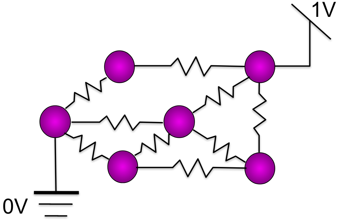
0V
1V
0.5
0.325
0.675
0.5
Potentials
Minimize
Minimize over x
Quadratic form
1V
0.5
0.5
0.325
0.675
0V
Graph Laplacian
System of linear equations
Applying the operator
creates some flow on the graph
: degree matrix
: adjacency matrix
Laplace Operator:
Heat Equation:
Informally, the Laplacian operator ∆ gives the difference between the average value of a function in the neighborhood of a point, and its value at that point. [wiki]
Graph diffusion:
Adjacency matrix
Normalized Laplacian
Random walk matrix
...
: degree matrix
: adjacency matrix
Pseudotime estimation**
Conos Annotation Transfer
Google PageRank algorithm*
k-NN Smoothing
(no picture)
Pseudotime estimation**
Conos Annotation Transfer
Google PageRank algorithm*
k-NN Smoothing
(no picture)
Can we re-write the Velocity equations on graph?
Eigenvalues:
Eigenvectors:
is a constant vector
Connected nodes have close vector values!
emb <- uwot::umap(
    X,
    metric="cosine",
    init="spectral"
)Normalized Laplacian
Normalized Laplacian Random walk matrix
Non-Normalized Laplacian
Laplacian
Degree matrix
Spectral drawing
Connected to Hitting Distances on graph
k-Means in spectral space approximates Minimum k-cut
Signal is given over the graph domain.
Derivative over an edge:
Gradient:
Local variation:
Laplacian:
Local variation:
Global variation:
Local variation:
Global variation:
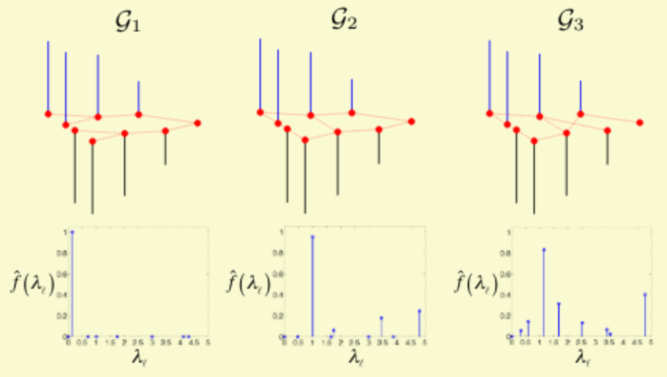
Filter size = k-hop on graph
Can we increase k?
Grid = Graph
Low-pass filter*
High-pass filter**
For eigenvector :
Global variation:
Inverse Fourier transform of :
Fourier transform of :
For eigenvector :
Global variation:
Inverse Fourier transform of :
Applying a
spectral filter :
It's just a low-pass filter
Low-pass filter*
High-pass filter**
def filterfunc(x):
    return (np.exp(-b * np.abs(x / graph.lmax - a)**p))

filt = pygsp.filters.Filter(graph, filterfunc)
EES = filt.filter(RES, method="chebyshev", order=50)Translation
Modulation
Convolution
Dilation
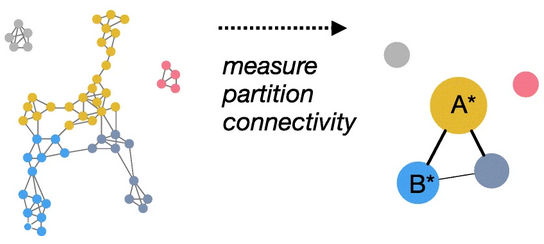
We can down-sample graph (both vertices and edges), preserving both graph topology and the signal!
We can do a better PAGA:
By Viktor Petukhov
Journal club presentation based on https://www.biorxiv.org/content/10.1101/532846v3 and https://ieeexplore.ieee.org/document/8347162


