Amazon CoRo June Update
Jun 19, 2025
Adam Wei
Agenda
- Algorithm Overview + Implementations
- Sim + Real Experiments
- GCS + RRT Experiments
- Next Directions
Part 1
Ambient Diffusion Recap
and Implementations
Ambient Diffusion
Learning from "clean" (\(p_0\)) and "corrupt" data (\(q_0\))
Learning in the high-noise regime
\(\exists \sigma_{min}\) s.t. \(d_\mathrm{TV}(p_{\sigma_{min}}, q_{\sigma_{min}}) < \epsilon\)
- Only use samples from \(q_0\) to train denoisers with \(\sigma > \sigma_{min}\)
- Corruption level of each datapoint determines its utility
\(\sigma=1\)
\(\sigma=0\)
\(\sigma=\sigma_{min}\)
Clean Data
Corrupt Data
Learning in the high-noise regime
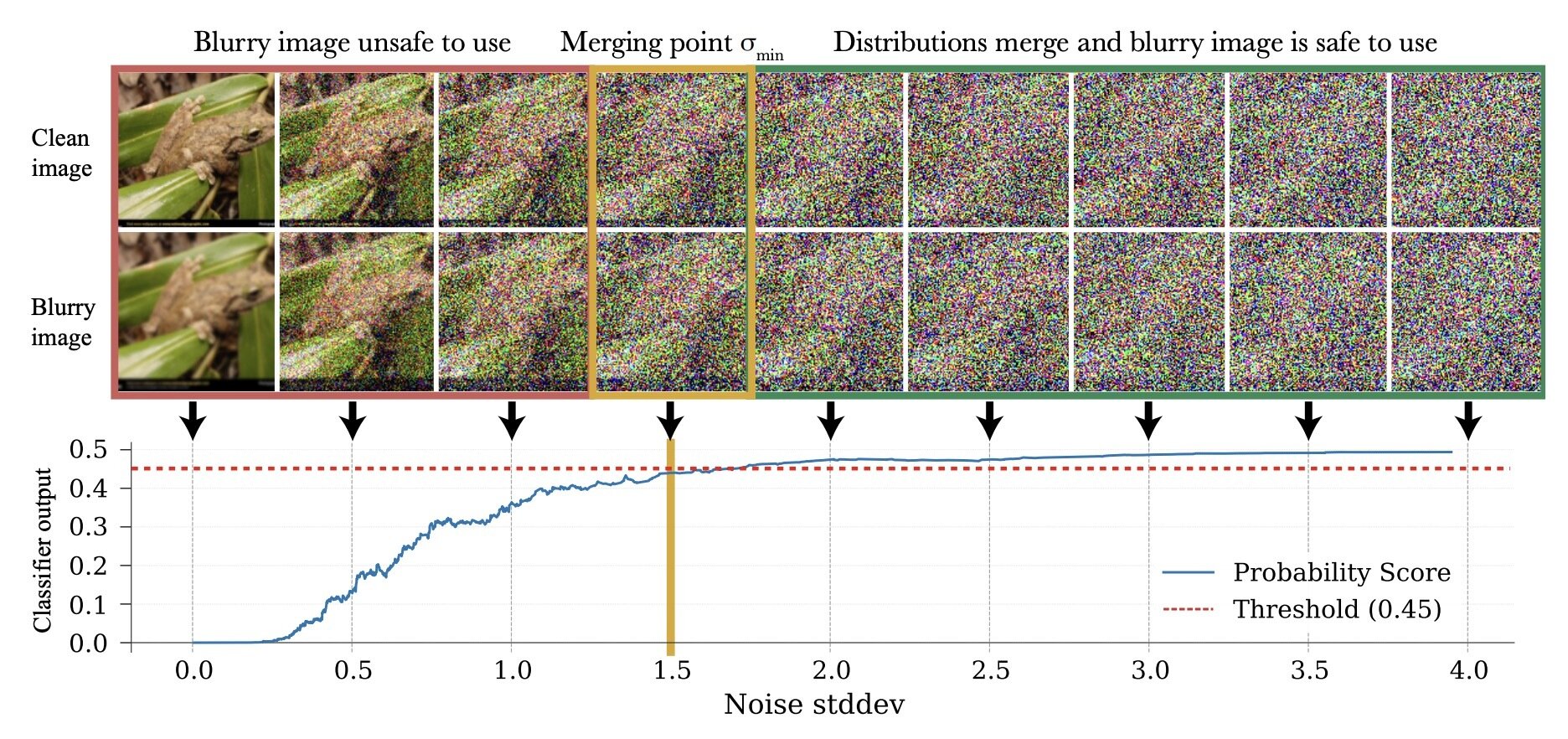
\(\exists \sigma_{min}\) s.t. \(d_\mathrm{TV}(p_{\sigma_{min}}, q_{\sigma_{min}}) < \epsilon\)
(in this example, \(\epsilon = 0.05\))
\(p_0\)
\(q_0\)
Learning in the high-noise regime
Factors that affect \(\sigma_{min}\):
- Similarity of \(p_0\), \(q_0\)
- Nature of the corruption from \(p_0\) to \(q_0\)
- Contracting \(q_{\sigma_{min}}\) towards \(p_{\sigma_{min}}\) "masks" corruption between \(p_0\) and \(q_0\)
... but also destroys useful signal
Contraction as masking
- Contracting \(q_{\sigma_{min}}\) towards \(p_{\sigma_{min}}\) "masks" corruption between \(p_0\) and \(q_0\)
... but also destroys useful signal
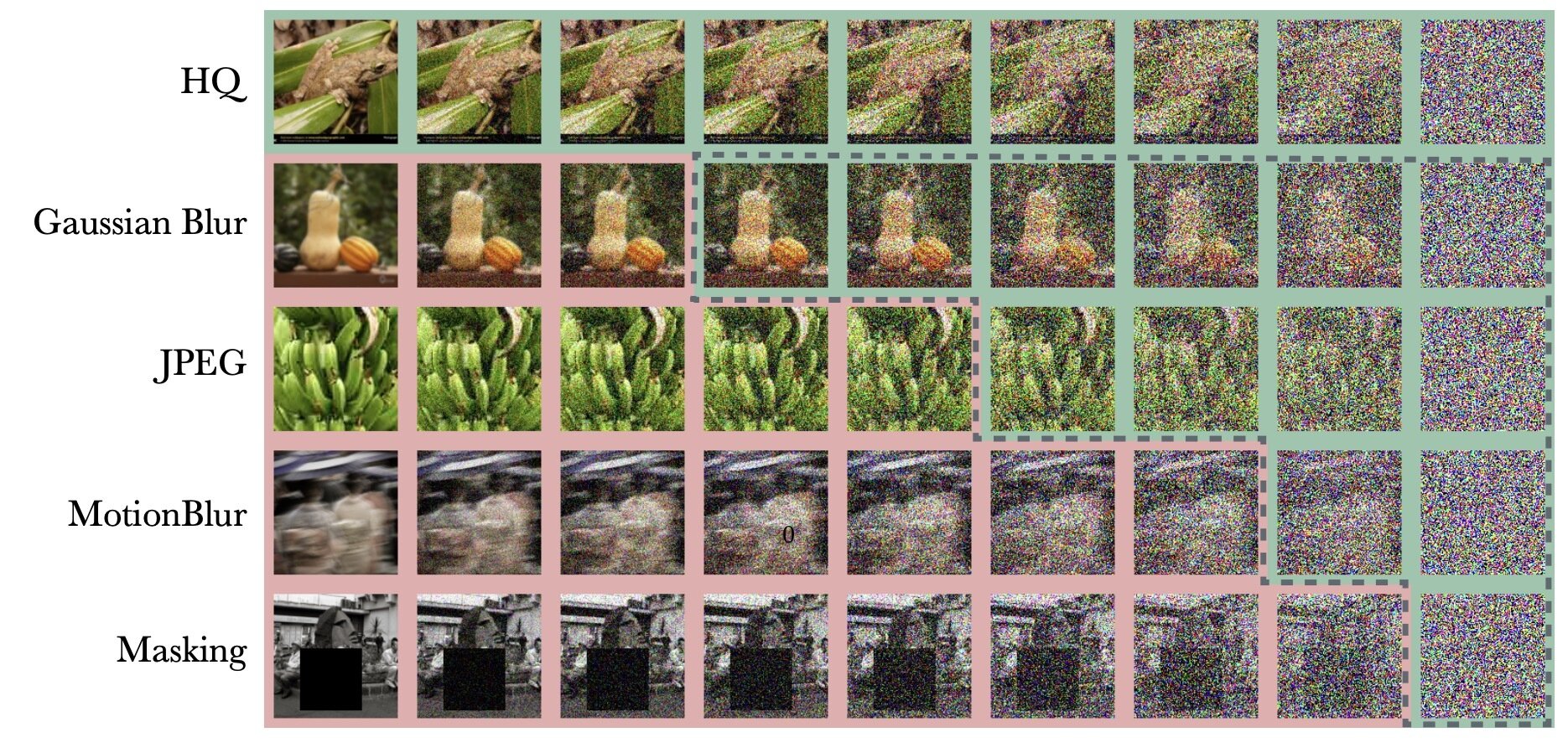
More info lost
Learning in the high-noise regime
\(\exists \sigma_{min}\) s.t. \(d_\mathrm{TV}(p_{\sigma_{min}}, q_{\sigma_{min}}) < \epsilon\)
- Only use samples from \(q_0\) to train denoisers with \(\sigma > \sigma_{min}\)
- Corruption level of each datapoint determines its utility
\(\sigma=1\)
\(\sigma=0\)
\(\sigma=\sigma_{min}\)
Denoising Loss
Denoising OR Ambient Loss
Loss Function (for \(x_0\sim q_0\))
\(\mathbb E[\lVert h_\theta(x_t, t) + \frac{\sigma_{min}^2\sqrt{1-\sigma_{t}^2}}{\sigma_t^2-\sigma_{min}^2}x_{t} - \frac{\sigma_{t}^2\sqrt{1-\sigma_{min}^2}}{\sigma_t^2-\sigma_{min}^2} x_{t_{min}} \rVert_2^2]\)
Ambient Loss
Denoising Loss
\(x_0\)-prediction
\(\epsilon\)-prediction
(assumes access to \(x_0\))
(assumes access to \(x_{t_{min}}\))
\(\mathbb E[\lVert h_\theta(x_t, t) - x_0 \rVert_2^2]\)
\(\mathbb E[\lVert h_\theta(x_t, t) - \epsilon \rVert_2^2]\)
\(\mathbb E[\lVert h_\theta(x_t, t) - \frac{\sigma_t^2 (1-\sigma_{min}^2)}{(\sigma_t^2 - \sigma_{min}^2)\sqrt{1-\sigma_t^2}}x_t + \frac{\sigma_t \sqrt{1-\sigma_t^2}\sqrt{1-\sigma_{min}^2}}{\sigma_t^2 - \sigma_{min}^2}x_{t_{min}}\rVert_2^2]\)
Sanity check: ambient loss \(\rightarrow\) denoising loss as \(\sigma_{min} \rightarrow 0\)
Experiments: Test all 4
Implementation Details
- Sample noise level first, then data points
- Ambient loss "buffer" for training stability
- Contract each datapoint once
- Other small details...
Implementation details: included for completeness...
Learning in the low-noise regime
Can use OOD data to learn in the low-noise regime...
... more on this next time
Part 2
Sim + Real Experiments
"Clean" Data
"Corrupt" Data
\(|\mathcal{D}_T|=50\)
\(|\mathcal{D}_S|=2000\)
Eval criteria: Success rate for planar pushing across 200 randomized trials
Datasets and Task
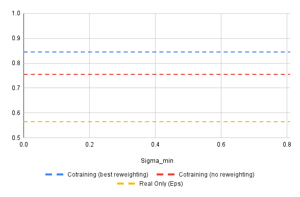
Results
Experiments
Choosing \(\sigma_{min}\): Swept several values on the dataset level
Loss function: Tried all 4 combinations of
{\(x_0\)-prediction, \(\epsilon\)-prediction} x {denoising, ambient}
Preliminary Observations
(will present best results on next slide)
- \(\epsilon\)-prediction > \(x_0\)-prediction and denosing > ambient loss
- Small (but non-zero) \(\sigma_{min}\) performed best
- Ambient diffusion scales slightly better with more sim data than cotraining
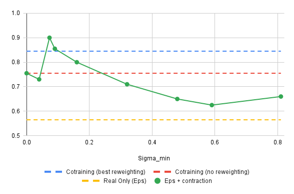
Results
\(|\mathcal{D}_S| = 50\), \(|\mathcal{D}_S| = 2000\), \(\epsilon\)-prediction with denoising loss
Results
\(|\mathcal{D}_S| = 50\), \(|\mathcal{D}_S| = 2000\), \(\epsilon\)-prediction with denoising loss
Part 3
Maze Experiments
Experiment: RRT vs GCS
GCS
(clean)
RRT
(clean)
Task: Cotrain on GCS and RRT data
Goal: Sample clean and smooth GCS plans
- Example of high frequency corruption
- Common in robotics
- Low quality teleoperation or data gen
Baselines
Success Rate: 50%
Average Jerk Squared: 7.5k
100 GCS Demos
Success Rate: 99%
Average Jerk Squared: 2.5k
4950 GCS Demos
Success Rate: 100%
Average Jerk Squared: 17k
4950 RRT Demos
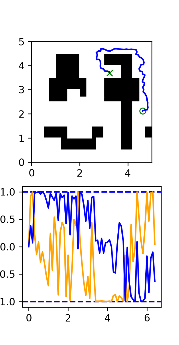
Cotraining vs Ambient Diffusion
Success Rate: 91%
Average Jerk Squared: 12.5k
Cotraining: 100 GCS Demos, 5000 RRT Demos, \(x_0\)-prediction
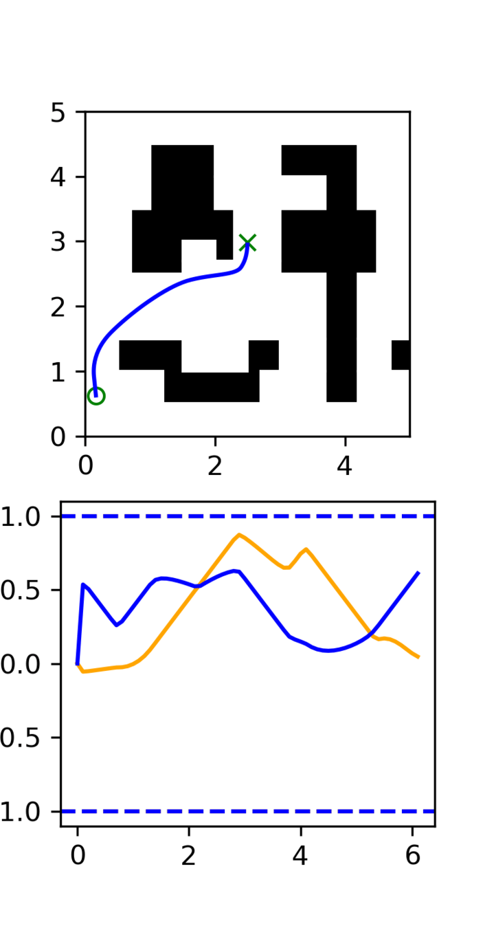
Success Rate: 98%
Average Jerk Squared: 5.5k
Ambient: 100 GCS Demos, 5000 RRT Demos, \(x_0\)-prediction ambient loss
See plots for qualitative results
Part 4
Next Experiments
North Star Goal
Main goal: Cotrain with ambient diffusion using internet data (Open-X, AgiBot, etc) and/or simulation data
... but first some "stepping stone" experiments
Stepping stone experiments are designed to
- Sanity check and debug implementations along the way
- Highlight and isolate specific components of the algorithm
- Improve exposition in the final paper
Experiment: Extend Maze to MP
Corrupt data: RRT/low quality data from 20-30 different environments
Clean data: GCS data from 2-3 environments
Performance metric: Success rate + smoothness metrics in seen/unseen environments
Purpose: Test learning in the high-noise regime
Experiment: Lu's Data
- Same task + plan structure, different robot embodiment
- Plans are high quality
- Trajectories (EE-space) have embodiment gap (lower quality)
Purpose: Test learning in the high-noise regime
Experiment: Bin Sorting
Task: Pick-and-place objects into specific bins
Clean Data: Demos with the correct logic
Corrupt Data: incorrect logic, Open-X, pick-and-place datasets, datasets with bins, etc
- Motions may be reasonable and informative
- But the decision making is incorrect
Purpose: Test learning in the low-noise regime
Experiment Document
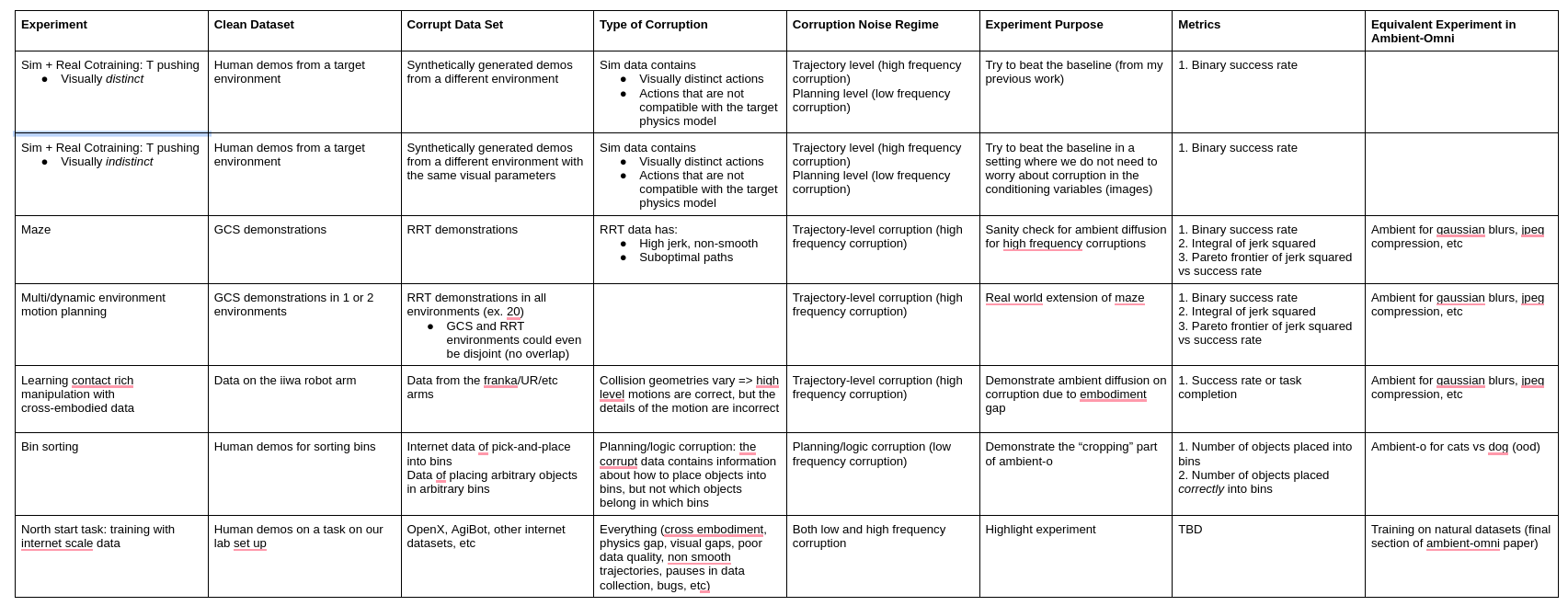
Details outlined in a google doc. Can share link privately if interested
Amazon CoRo July
By weiadam
Amazon CoRo July
Slides for my talk at the Amazon CoRo Symposium 2025. For more details, please see the paper: https://arxiv.org/abs/2503.22634


