Learning From Corrupt/Noisy Data
RLG Long Talk
May 2, 2025
Adam Wei
Agenda
- Motivation
- Ambient Diffusion
- Interpretation
- Experiments
... works in progress
Part 1
Motivation
Sources of Robot Data
Open-X
expert robot teleop
robot teleop
simulation

Goal: sample "high-quality" trajectories for your task
Train on entire spectrum to learn "high-level" reasoning, semantics, etc
"corrupt"
"clean"
Corrupt Data
Corrupt Data
Clean Data
Computer Vision
Language

Poor writing, profanity, toxcity, grammar/spelling errors, etc


👀
Research Questions
- How can we learn from both clean and corrupt data?
- Can these algorithms be adapted for robotics?

Giannis Daras
Part 2a
Ambient Diffusion
Diffusion: Sample vs Epsilon Prediction
\mathbb E[\lVert h_\theta(x_t, t) - x_0 \rVert_2^2]
\mathbb E[\lVert \epsilon_\theta(x_t, t) - \epsilon \rVert_2^2]
Epsilon prediction:
Sample prediction:
affine transform
h^*(x_t, t) = \mathbb E_{p_{X_0|X_t=x_t}}[X_0 | X_t = x_t]
Diffusion: VP vs VE
X_t = \sqrt{1-\sigma_t^2}X_0 + \sigma_t Z
Variance preserving:
Variance exploding:
X_t = X_0 + \sigma_t Z
Variance exploding and sample-prediction simplify analysis
... analysis can be extended to DDPM
Ambient Diffusion
Assumptions
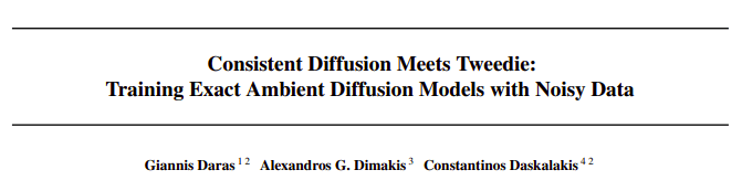
1. Each corrupt data point contains additive gaussian noise up to some noise level \(t_n\)
X_{t_n} = X_0 + \sigma_{t_n} Z
X_0\sim p_0,\ Z\sim \mathcal N(0, I)
\(t=0\)
\(t=T\)
\(t=t_n\)
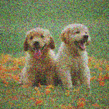


Corrupt data: \(X_{t_n} = X_0 + \sigma_{t_n} Z\)
Ambient Diffusion
Assumptions
1. Each corrupt data point contains additive gaussian noise up to some noise level \(t_n\)
2. \(t_n\) is known for each dataset or datapoint
\(t=0\)
\(t=T\)
\(t=t_n\)
Corrupt data: \(X_{t_n} = X_0 + \sigma_{t_n} Z\)
Naive Diffusion
\(t=0\)
\(t=T\)
\(t=t_n\)
noise
denoise
\mathbb E[\lVert h_\theta(x_t, t) - x_{t_n} \rVert_2^2]
\implies h_\theta^*(x_t, t) = \mathbb E[X_{t_n} | X_t = x_t]
x_t = x_{t_n} + \sqrt{\sigma_t^2 - \sigma_{t_n}^2}Z
Forward Process
Backward Process
\implies h_\theta^*(x_t, t) = \mathbb E[X_{t_n} | X_t = x_t]
Can we do better?
\(t=0\)
\(t=T\)
\(t=t_n\)
noise
denoise
h_\theta^*(x_t, t) = \mathbb E[X_0 | X_t = x_t]
x_t = x_{t_n} + \sqrt{\sigma_t^2 - \sigma_{t_n}^2}Z
Forward Process
Backward Process
Can we do better?
\(t=0\)
\(t=T\)
\(t=t_n\)
noise
denoise
How can we learn \(h_\theta^*(x_t, t) = \mathbb E[X_0 | X_t = x_t]\) using noisy samples \(X_{t_n}\)?
Ambient Diffusion
\mathbb E[\lVert \frac{\sigma_t^2 - \sigma_{t_n}^2}{\sigma_t^2} h_\theta(x_t,t) + \frac{\sigma_{t_n}^2}{\sigma_t^2}x_t - x_{t_n} \rVert_2^2]
\implies h_\theta^*(x_t, t) = \mathbb E[X_0 | X_t = x_t]
Ambient Loss
Note that this loss does not require access to \(x_0\)
How can we learn \(h_\theta^*(x_t, t) = \mathbb E[X_0 | X_t = x_t]\) using noisy samples \(X_{t_n}\)?
\mathbb E[\lVert h_\theta(x_t,t) - x_0 \rVert_2^2]
Diffusion Loss
No access to \(x_0\)
Ambient Diffusion
We can learn \(\mathbb E[X_0 | X_t=x_t]\) using only corrupted data!
Remarks
- From any given \(x_{t_n}\), you cannot recover \(x_0\)
- Given \(p_{X_{t_n}}\), you can compute \(p_{X_0}\)
- "No free lunch": learning \(p_{X_0}\) from \(X_{t_n}\) requires more samples than learning from clean data \(X_0\)
\mathbb E[\lVert \frac{\sigma_t^2 - \sigma_{t_n}^2}{\sigma_t^2} h_\theta(x_t,t) + \frac{\sigma_{t_n}^2}{\sigma_t^2}x_t - x_{t_n} \rVert_2^2]
Proof: "Double Tweedies"
\(X_{t} = X_0 + \sigma_{t}Z\)
\(X_{t} = X_{t_n} + \sqrt{\sigma_t^2 - \sigma_{t_n}^2}Z\)
\(\nabla \mathrm{log} p_t(x_t) = \frac{\mathbb E[X_0|X_t=x_t]-x_t}{\sigma_t^2}\)
\(\nabla \mathrm{log} p_t(x_t) = \frac{\mathbb E[X_{t_n}|X_t=x_t]-x_t}{\sigma_t^2-\sigma_{t_n}^2}\)
\mathbb E[X_0 | X_t=x_t] = \frac{\sigma_t^2}{\sigma_t^2 - \sigma_{t_n}^2}\mathbb E[X_{t_n} | X_t=x_t] - \frac{\sigma_{t_n}^2}{\sigma_t^2 - \sigma_{t_n}^2}x_t
(Tweedies)
(Tweedies)
Proof: "Double Tweedies"
\(g_\theta(x_t,t) := \frac{\sigma_t^2 - \sigma_{t_n}^2}{\sigma_t^2} h_\theta(x_t,t) + \frac{\sigma_{t_n}^2}{\sigma_t^2}x_t\).
\mathcal L = \mathbb E [\lVert \frac{\sigma_t^2 - \sigma_{t_n}^2}{\sigma_t^2} h_\theta(x_t,t) + \frac{\sigma_{t_n}^2}{\sigma_t^2}x_t - x_{t_n} \rVert_2^2]
Ambient loss:
\implies \mathcal L = \mathbb E [\lVert g_\theta(x_t, t) - x_{t_n} \rVert_2^2]
\implies g_{\theta}^*(x_t,t) = \mathbb E [X_{t_n} | X_t = x_t]
Proof: "Double Tweedies"
\implies g_{\theta}^*(x_t,t) = \mathbb E [X_{t_n} | X_t = x_t]
\(\frac{\sigma_t^2 - \sigma_{t_n}^2}{\sigma_t^2} h_\theta^*(x_t,t) + \frac{\sigma_{t_n}^2}{\sigma_t^2}x_t = \mathbb E [X_{t_n} | X_t = x_t]\)
\begin{aligned}
h_\theta^*(x_t,t) &= \frac{\sigma_t^2}{\sigma_t^2 - \sigma_{t_n}^2}\mathbb E[X_{t_n} | X_t=x_t] - \frac{\sigma_{t_n}^2}{\sigma_t^2 - \sigma_{t_n}^2}x_t \\
&= \mathbb E[X_0 | X_t=x_t]
\end{aligned}
(from double Tweedies)
\(\implies\)
\(\implies\)
(definition of \(g_\theta\))
Training Algorithm
For each data point:
Clean data: \(t\in (0, T]\)
\(x_t = x_0 + \sigma_t z\)
\(\mathbb E[\lVert h_\theta(x_t, t) - x_0 \rVert_2^2]\)
Forward process:
Backprop:
Corrupt data
\(t\in (t_n, T]\)
\(x_t = x_{t_n} + \sqrt{\sigma_t^2-\sigma_{t_n}^2} z_2\)
\(\mathbb E[\lVert \frac{\sigma_t^2 - \sigma_{t_n}^2}{\sigma_t^2} h_\theta(x_t,t) + \frac{\sigma_{t_n}^2}{\sigma_t^2} - x_{t_n} \rVert_2^2]\)
Ambient Diffusion
\(t=0\)
\(t=T\)
\(t=t_n\)
\(\mathbb E[\lVert h_\theta(x_t, t) - x_0 \rVert_2^2]\)
\(\mathbb E[\lVert \frac{\sigma_t^2 - \sigma_{t_n}^2}{\sigma_t^2} h_\theta(x_t,t) + \frac{\sigma_{t_n}^2}{\sigma_t^2}x_t - x_{t_n} \rVert_2^2]\)
Use clean data to learn denoisers for \(t\in(0,T]\)
Use corrupt data to learn denoisers for \(t\in(t_n,T]\)
Part 2b
Ambient Diffusion w/ Contraction
Protein Folding Case Study
Case Study: Protein Folding
Assumptions
1. Each corrupt data point contains additive gaussian noise up to some noise level \(t_n\)
2. \(t_n\) is known for each dataset or datapoint
\(t=0\)
\(t=T\)
\(t=t_n\)
Corrupt data: \(X_{t_n} = X_0 + \sigma_{t_n} Z\)
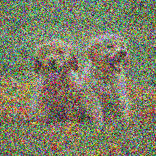
Case Study: Protein Folding
Corrupt Data
Clean Data


+ 5 years
=
~100,000 solved protein structures
200M+ protein structures
Case Study: Protein Folding
Corrupt Data
Clean Data
\(X_0^{corrupt} \neq X_0^{clean} + \sigma_{t_n} Z\)
Breaks both assumptions:
- Corruption is not additive Gaussian noise
- Don't know \(t_n\) for each AlphaFold protein
\(X_0^{clean}\)
\(X_0^{corrupt}\)
Corrupt Data
Clean Data
Corrupt Data + Noise

For sufficiently high \(t_n\): \(X_{t_n}^{corrupt} = X_0^{corrupt} + \sigma_{t_n} Z \approx X_0^{clean} + \sigma_{t_n} Z\)
\(X_{t_n}^{corrupt} = X_0^{corrupt} + \sigma_{t_n} Z\)
Key idea: Corrupt data further with Gaussian noise
Assumption 1: Contraction


\(X_0^{clean}\)
\(X_0^{corrupt}\)
\(X_{t_n}^{corrupt}\)
Key idea: Corrupt data further with Gaussian noise
For sufficiently high \(t_n\): \(X_{t_n}^{corrupt} = X_0^{corrupt} + \sigma_{t_n} Z \approx X_0^{clean} + \sigma_{t_n} Z\)

\(x_0^{clean}\)
\(x_0^{corrupt}\)
\(t=0\)
\(t=T\)
\(t=t_n\)
Assumption 1: Contraction
For sufficiently high \(t_n\): \(X_{t_n}^{corrupt} \approx X_0^{clean} + \sigma_{t_n} Z\)
\(P_{Y|X}\)
\(Y = X + \sigma_{t_n} Z\)
\(P_{X_0}^{clean}\)
\(Q_{X_0}^{corrupt}\)
\(P_{X_{t_n}}^{clean}\)
\(Q_{X_{t_n}}^{corrupt}\)
D(P_{X_0}^{clean}||Q_{X_0}^{corrupt}) \geq D(P_{X_{t_n}}^{clean}||Q_{X_{t_n}}^{corrupt})
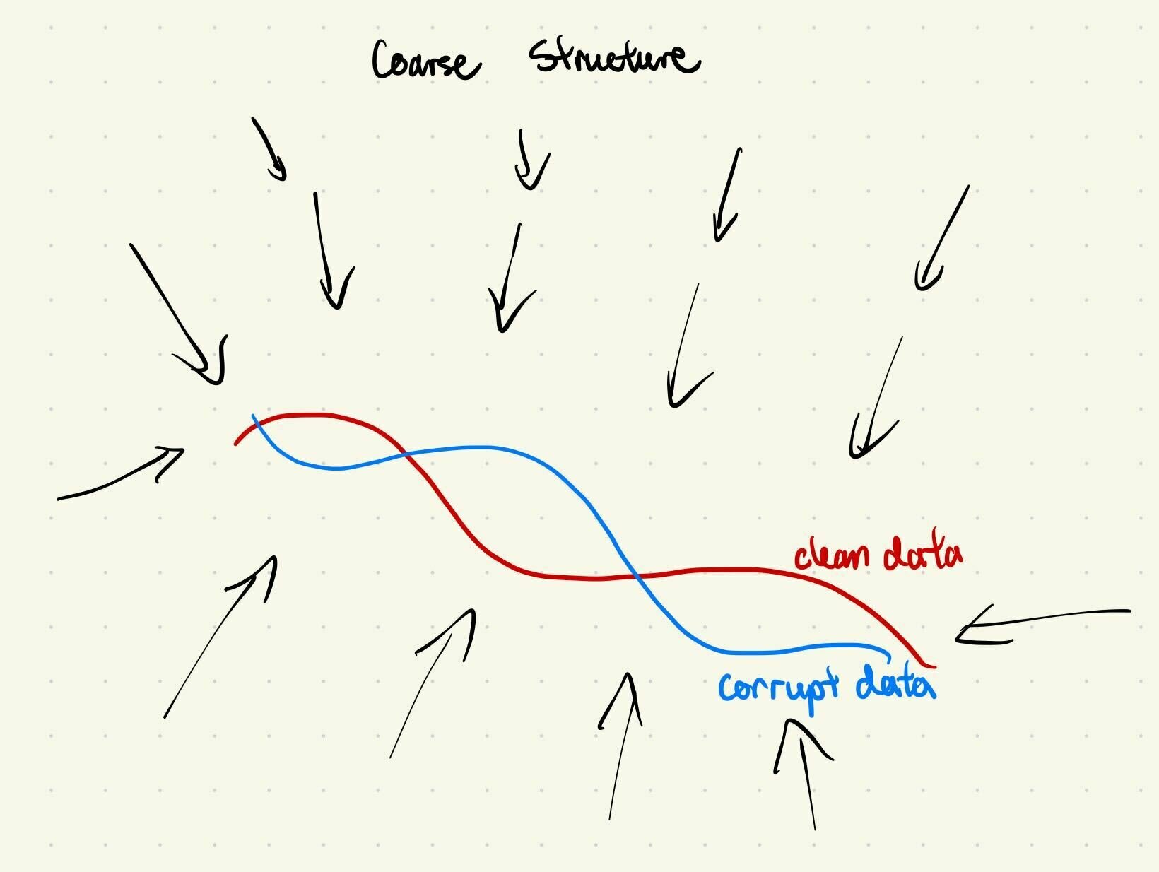
Assumption 1: Contraction
\(\implies\) Adding noise makes the corruption appear Gaussian (Assumption 1)
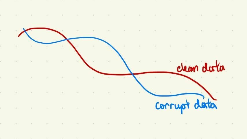
- Clean and corrupt data share coarse structure
- Adding noise masks high-frequency differences, preserves low frequency similarities
\(x_0^{clean}\)
\(x_0^{corrupt}\)
\(t=0\)
\(t=T\)
\(t=t_n\)
Assumption 1: Intuition
Assumption 2: Finding \(t_n\)
1. Train a "clean" vs "corrupt" classifier for all \(t \in [0, T]\)
2. For each corrupt data point, increase noise until the classification accuracy drops. This is \(t_n\).
\(x_0^{clean}\)
\(x_0^{corrupt}\)
\(t=0\)
\(t=T\)
\(t=t_n\)
Training Algorithm
For each data point:
Clean data
\(x_t = x_0 + \sigma_t z\)
\(\mathbb E[\lVert h_\theta(x_t, t) - x_0 \rVert_2^2]\)
Forward process:
Backprop:
Corrupt data
\(x_t = x_{t_n} + \sqrt{\sigma_t^2-\sigma_{t_n}^2} z_2\)
\(x_{t_n} = x_0 + \sigma_{t_n} z_1\)
Contract data:
\(\mathbb E[\lVert \frac{\sigma_t^2 - \sigma_{t_n}^2}{\sigma_t^2} h_\theta(x_t,t) + \frac{\sigma_{t_n}^2}{\sigma_t^2} - x_{t_n} \rVert_2^2]\)
Part 3
Interpretations
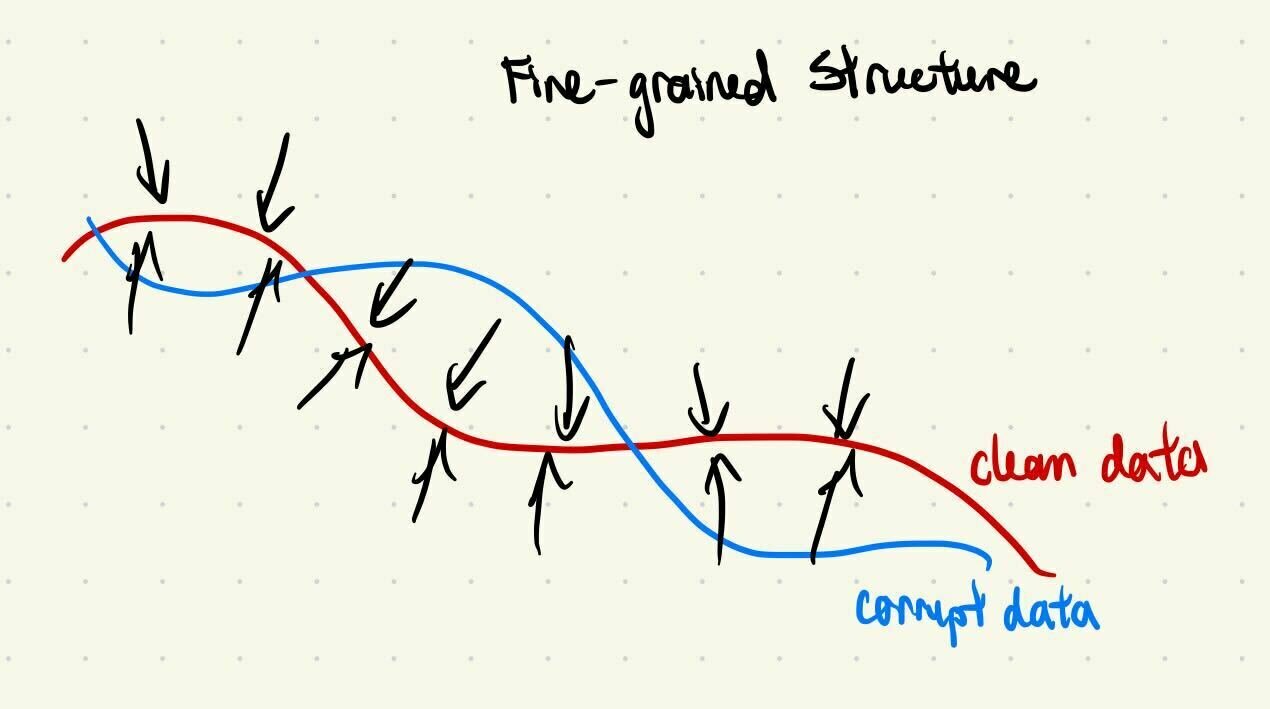
Frequency Domain Interpretation
Diffusion is AR sampling in the frequency domain
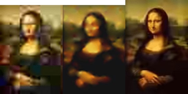
Frequency Domain Interpretation*
\(t=0\)
\(t=T\)
\(t=t_n\)
Low Frequency
High Frequency
Coarse Structure
Fine-grained Details
* assuming power spectral density of data is decreasing
Frequency Domain Interpretation
\(t=0\)
\(t=T\)
\(t=t_n\)
\(\mathbb E[\lVert h_\theta(x_t, t) - x_0 \rVert_2^2]\)
\(\mathbb E[\lVert \frac{\sigma_t^2 - \sigma_{t_n}^2}{\sigma_t^2} h_\theta(x_t,t) + \frac{\sigma_{t_n}^2}{\sigma_t^2}x_t - x_{t_n} \rVert_2^2]\)
Low Freq
High Freq
Clean & corrupt data share the same "coarse structure"
Learn coarse structure from all data
Learn fine-grained details from clean data only
i.e. same low frequency features
Clean Data
Corrupt Data
Robotics Hypothesis
Hypothesis: Robot data shares low-frequency features, but differ in high frequency features
Clean & corrupt data share the same "coarse structure"
i.e. same low frequency features
Low Frequency
- Move left or right
- Semantics & language
- High-level decision making
Learn with Open-X, AgiBot, sim, clean data, etc
High Frequency
- Environment physics/controls
- Task-specific movements
- Specific embodiment
Learn from clean task-specific data
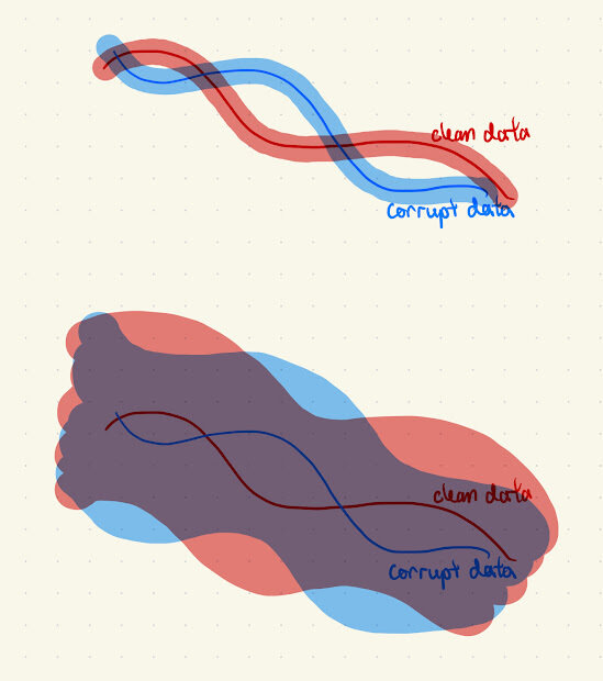
"Manifold" Interpretation
Diffusion is Euclidean projection onto the data manifold
Assumption: The clean and corrupt data manifolds lie in a similar part of space, but differ in shape
"Manifold" Interpretation
Diffusion is Euclidean projection onto the data manifold
Large \(\sigma_t\)
Both clean and corrupt data project to close to the clean data manifold
"Manifold" Interpretation
Diffusion is Euclidean projection onto the data manifold
Small \(\sigma_t\)
Use clean data to project onto the clean data manifold
Part 4
Robotics??
Robotics
Open-X
expert robot teleop
robot teleop
simulation
"corrupt"
"clean"
Start by exploring ideas inspired by Ambient Diffusion on sim-and-real cotraining
Robotics: Sim-and-Sim Cotraining
Corrupt Data (Sim): \(\mathcal D_S\)
Clean Data (Real): \(\mathcal D_T\)
Replayed GCS plans in Drake
Sources of corruption: (non-Gaussian...)
- Physics gap
- Visual gap
- Action gap
Teleoperated demos in a target-sim environment
... sorry no video :(
Robotics Idea 1: Modified Diffusion
- Assume all simulated data points in \(\mathcal D_S\) are corrupted with some fixed level \(t_n\)
- For \(t > t_n\): train denoisers with clean and corrupt data
- For \(t \leq t_n\): train denoisers with only clean data
- Use regular DDPM loss (i.e. not ambient loss)
- Since the sim_data \(\neq\) real_data + noise
Training:
Robotics Idea 1: Modified Diffusion
\(t=0\)
\(t=T\)
\(t=t_n\)
\(\mathbb E[\lVert h_\theta(x_t, t) - x_0^{clean} \rVert_2^2]\)
\(\mathbb E[\lVert h_\theta(x_t, t) - x_0^{corrupt} \rVert_2^2]\)
Low Freq
High Freq
Learn with all data
Learn with clean data
Clean Data
Corrupt Data
Intuition: mask out high-frequency components of "corrupt" data
Robotics Idea 1
Robotics Idea 2: Ambient w/o Contraction
\(t=0\)
\(t=T\)
\(t=t_n\)
\(\mathbb E[\lVert h_\theta(x_t, t) - x_0^{clean} \rVert_2^2]\)
Low Freq
High Freq
Learn with all data
Learn with clean data
Clean Data
Corrupt Data
Assume \(X_0^{corrupt} = X_{t_n}^{clean} = X_0^{clean} + \sigma_{t_n} Z\)
(NOT TRUE)
\(\mathbb E[\lVert \frac{\sigma_t^2 - \sigma_{t_n}^2}{\sigma_t^2} h_\theta(x_t,t) + \frac{\sigma_{t_n}^2}{\sigma_t^2}x_t - x_0^{corrupt} \rVert_2^2]\)
Robotics Idea 1
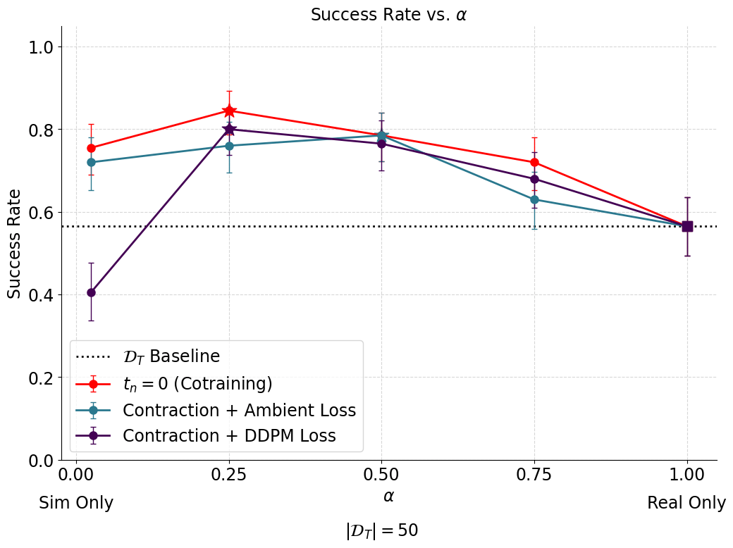
Results: Idea 1
- 50 clean (real) demos
- 2000 corrupt (sim) demos
- 200 trials each
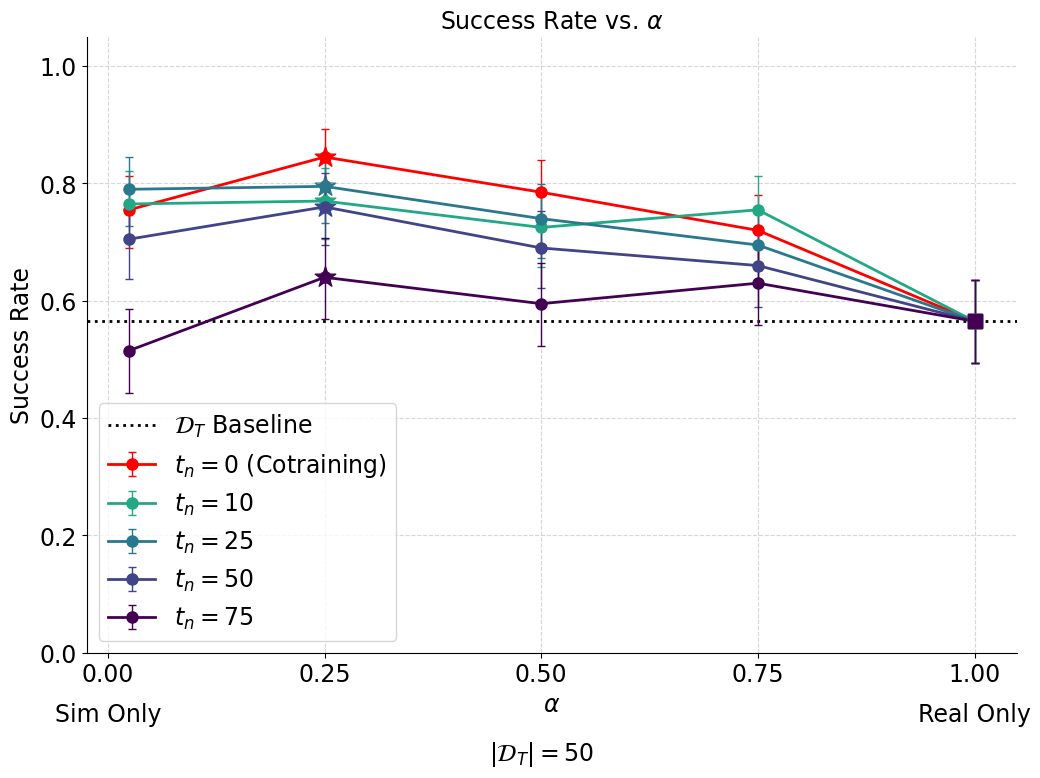
Results are currently worse than the cotraining baseline :(
Robotics Idea 1
Discussion: Idea 1
- Ambient diffusion loss rescaling
- Real and sim data are too similar at all noise levels
- \(\implies\) no incentive to mask out high-frequency components of "corrupt" data
- Will potentially find more success using Open-X, AgiBot, etc
- Image conditioning is sufficient to disambiguate sampling from clean (real) vs corrupt (sim)
\(\mathbb E[\lVert \frac{\sigma_t^2 - \sigma_{t_n}^2}{\sigma_t^2} h_\theta(x_t,t) + \frac{\sigma_{t_n}^2}{\sigma_t^2}x_t - x_{t_n} \rVert_2^2]\)
\(\mathbb E[\lVert h_\theta(x_t,t) + \frac{\sigma_{t_n}^2}{\sigma_t^2-\sigma_{t_n}^2}x_t - \frac{\sigma_t^2}{\sigma_t^2 - \sigma_{t_n}^2}x_{t_n} \rVert_2^2]\)
Ambient Loss
"Rescaled" Ambient Loss
... blows up for small \(\sigma_t\)
Robotics Idea 1
Discussion: Idea 1
- Ambient diffusion loss rescaling
- Real and sim data are too similar at all noise levels
- \(\implies\) no incentive to mask out high-frequency components of "corrupt" data
- Will potentially find more success using Open-X, AgiBot, etc
- Image conditioning is sufficient to disambiguate sampling from clean (real) vs corrupt (sim)
- Hyperparameter sweep
Robotics Idea 1
Results: Idea 2
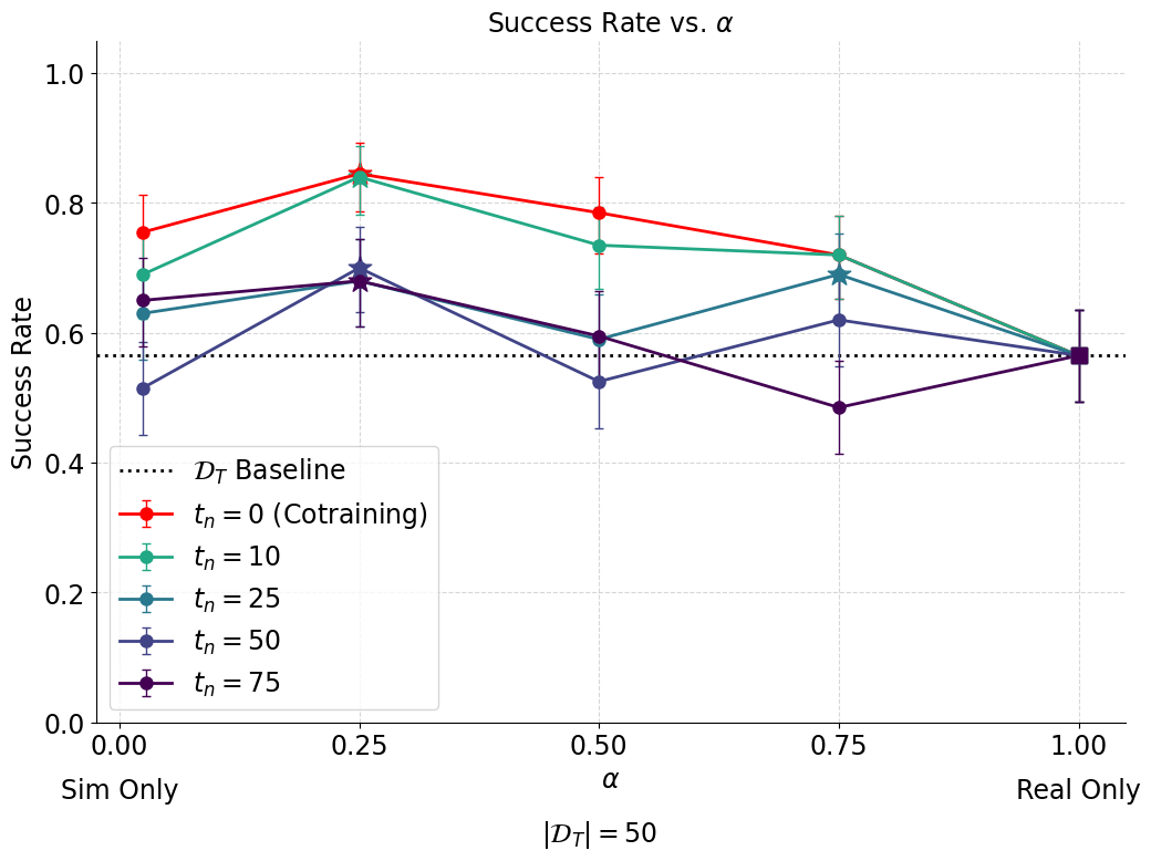
Worse than idea 1, but this was expected
Assume \(X_0^{corrupt} = X_{t_n}^{clean} = X_0^{clean} + \sigma_{t_n} Z\)
(NOT TRUE)
Robotics Idea 1
Idea 3: Ambient w/ Contraction
1. Train a binary classifier to distinguish sim vs real actions
2. Use the classifier to find \(t_n\) for all sim actions in \(\mathcal D_S\)
3. Noise all sim actions to \(t_n\):
\(X_{t_n}^{corrupt} = X_0^{corrupt} + \sigma_{t_n} Z\)
\(\approx X_0^{clean} + \sigma_{t_n} Z\)
4. Train with ambient diffusion and \(t_n\) per datapoint
*same algorithm as SOTA protein folding
Robotics Idea 1
Idea 3: Ambient w/ Contraction
1. Train a binary classifier to distinguish sim vs real actions
2. Use the classifier to find \(t_n\) for all sim actions in \(\mathcal D_S\)
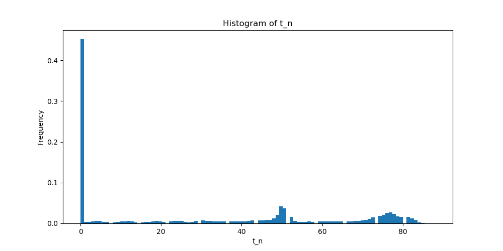
\(t_n\) = 0 for 40%+ of action sequences... \(\implies\) sim data is barely corrupt
Robotics Idea 1
Idea 3: Ambient w/ Contraction
Robotics Idea 1
Idea 4: ... but first recall idea 1
\(t=0\)
\(t=T\)
\(t=t_n\)
\(\mathbb E[\lVert h_\theta(x_t, t) - x_0^{clean} \rVert_2^2]\)
\(\mathbb E[\lVert h_\theta(x_t, t) - x_0^{corrupt} \rVert_2^2]\)
Low Freq
High Freq
Learn with all data
Learn with clean data
Clean Data
Corrupt Data
Robotics Idea 1
Idea 4: Different \(\alpha_t\) per \(t\in (0, T]\)
\(t=0\)
\(t=T\)
Low Freq
High Freq
Clean Data
Corrupt Data
- Train with different data mixtures \(\alpha_t\) at different noise levels
\(\mathbb E[\lVert h_\theta(x_t, t) - x_0^{clean} \rVert_2^2]\)
\(\mathbb E[\lVert h_\theta(x_t, t) - x_0^{corrupt} \rVert_2^2]\)
\(\alpha_T\)
\(\alpha_0\)
Robotics Idea 1
Idea 4: Different \(\alpha_t\) per \(t\in (0, T]\)
\(D(\red{p^{clean}_{\sigma_t}}||\blue{p^{corrupt}_{\sigma_t}})\) is large
\(\implies\) sample more clean data
Low noise levels
(small \(\sigma_t\))
High noise levels
(large \(\sigma_t\))
\(D(\red{p^{clean}_{\sigma_t}}||\blue{p^{corrupt}_{\sigma_t}})\) is small
\(\implies\) sample more corrupt data
Robotics Idea 1
Next Directions
- Try to improve results for all 4 ideas on planar pushing
- Try ambient diffusion related ideas for cotraining from Open-X or AgiBot
Robotics Idea 1
Thoughts
Motivating ideas for ambient diffusion
- Noise as partial masking (mask out high frequency corruption)
- Clean and corrupt distributions are more similar at high noise levels
Motivating ideas could be useful for robotics, but the exact Ambient Diffusion algorithm might not??
Thank you!
Spring 2025 Long Talk
By weiadam


