cog sci 131 section
week 02/21/22
by yuan meng
agenda
- perceptron from scratch
- load local images in jupyter
- hw5 prompt walkthrough
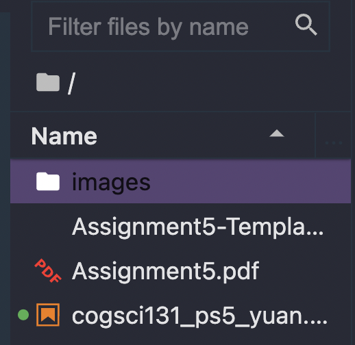
classify L vs. 7
- describe how you tell them apart
- "L": top right is empty (0) or lower left is not empty (1)
- "7": lower left is empty (0) or top right is not empty (1)
- can you "hand-pick" the weights W = [w1, w2, w3, w4]?
- L: w1 + 0 + w3 + w4 < 0
- 7: w1 + w2 + 0 + w4 > 0
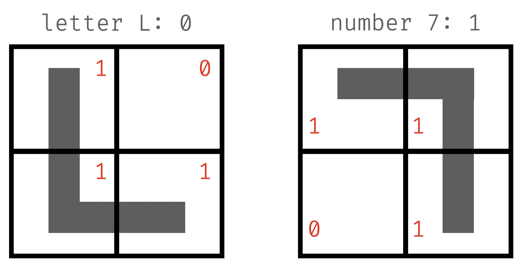
X: [1, 0, 1, 1]
not "pulling punches" 👉 set to around 0
\mathbf{x}\cdot\mathbf{W} < 0
X: [1, 1, 0, 1]
\mathbf{x}\cdot\mathbf{W} \geq 0
likely negative
👉 < - (w1 + w4)
likely positive
👉 > w1 + w4
class label: 0
class label: 1
classify L vs. 7
- initialization: start with random weights, W = [0.5, 0.9, -0.3, 0.5]
-
training: "see" an example of "L"
- perception is "blind" 👉 use weights to "see"
- dot product > 0 👉 classify as "7"
- wrong❗️updating is needed
-
update: increase or decrease W?
- how to adjust: decrease, b/c predicted value is too large
- new weights: subtract x from W
\mathbf{W}\cdot\mathbf{x} = 0.5 \times 1 + 0.9 \times 0 -0.3 \times 1 + 0.5 \times 1 = 0.7
class label: 0
\mathbf{W}-\mathbf{x} \\ = [0.5 - 1, 0.9 - 0, -0.3 - 1, 0.5 - 1] \\ = [-0.5, 0.9, -1.3, -0.5]
classify L vs. 7
- weights: [-0.5, 0.9, -1.3, -0.5]
-
training: "see" an example of "7"
- use new weights to classify
- dot product < 0 👉 classify as "L"
- wrong❗️updating is needed
-
update: increase or decrease W?
- how to adjust: increase, b/c predicted value is too small
- new weights: add x to W
\mathbf{W}\cdot\mathbf{x} = -0.5 \times 1 + 0.9 \times 1 -1.3 \times 0 - 0.5 \times 1 = -0.1
class label: 1
\mathbf{W}-\mathbf{x} \\ = [-0.5 + 1, 0.9 + 1, -1.3 + 0, - 0.5 + 1] \\ = [0.5, 1.9, -1.3, 0.5]
classify L vs. 7
- weights: [0.5, 1.9, -1.3, 0.5]
-
training: "see" an example of "L"
- use new weights to classify
- dot product < 0 👉 classify as "L"
- correct❗️no need to update
-
train on more examples...
- evaluation metrics: accuracy (# of correct/# test cases), precision (actually yes/say yes), recall (say yes/actually yes), log-loss...
- when to stop: "train just enough" (early stopping)
\mathbf{W}\cdot\mathbf{x} = 0.5 \times 1 + 1.9 \times 0 -1.3 \times 1 + 0.5 \times 1 = -0.3
class label: 0
🥳
used in hw5
read local images in jupyter
- unzip "Assignment5-images.zip" 👉 creates folder "images"
- run your notebook in the parent directory
# dimension of all images
DIM = (28, 28)
# flattened imahe
N = DIM[0] * DIM[1]

def load_image_files(n, path="images/"):
    """loads images of given digit and returns a list of vectors"""
    # initialize empty list to collect vectors
    images = []
    # read files in the path
    for f in sorted(os.listdir(os.path.join(path, str(n)))):
        p = os.path.join(path, str(n), f)
        if os.path.isfile(p):
            i = np.loadtxt(p)
            # check image dimension
            assert i.shape == DIM
            # flatten i into a single vector
            images.append(i.flatten())
    return images

# load images of '0' and '1'
img1 = load_image_files(0)
img0 = load_image_files(1)
1brown3blue author on working w/ images (in julia, but well explained)
hw5 prompts
notes & tips
- useful functions for this homework
- manipulate matrices: arr2d.flatten(), np.reshape(arr1d, (dim1, dim2)), np.dot(m1, m2)
- visualize matrices: image 👉 ax.imshow(m); heatmap 👉ax.imshow(m, cmap="Blues")
- sample from a list: random.sample(l, n_samples)
- labels: to classify digit a vs. b, label former as 0 and latter as 1 👉 don't use actual numbers as labels ( 1, 2, 3...)
- how long to train: plot accuracy against # of training steps (epochs) to see when the curve flattens out
arr2d: name of your 2d numpy array
arr1d: name of your 1d numpy array
two numpy arrays of same length
array to plot (q3: weights; q5: accuracies)
dimension of target 2d array
cogsci131_02_21_section
By Yuan Meng


