cog sci 131 section
week 04/04/22
by yuan meng
agenda
- visualize bayesian inference
- implement bayesian workflow
- hw8 prompt walkthrough
- optional fun: modern-day bayes
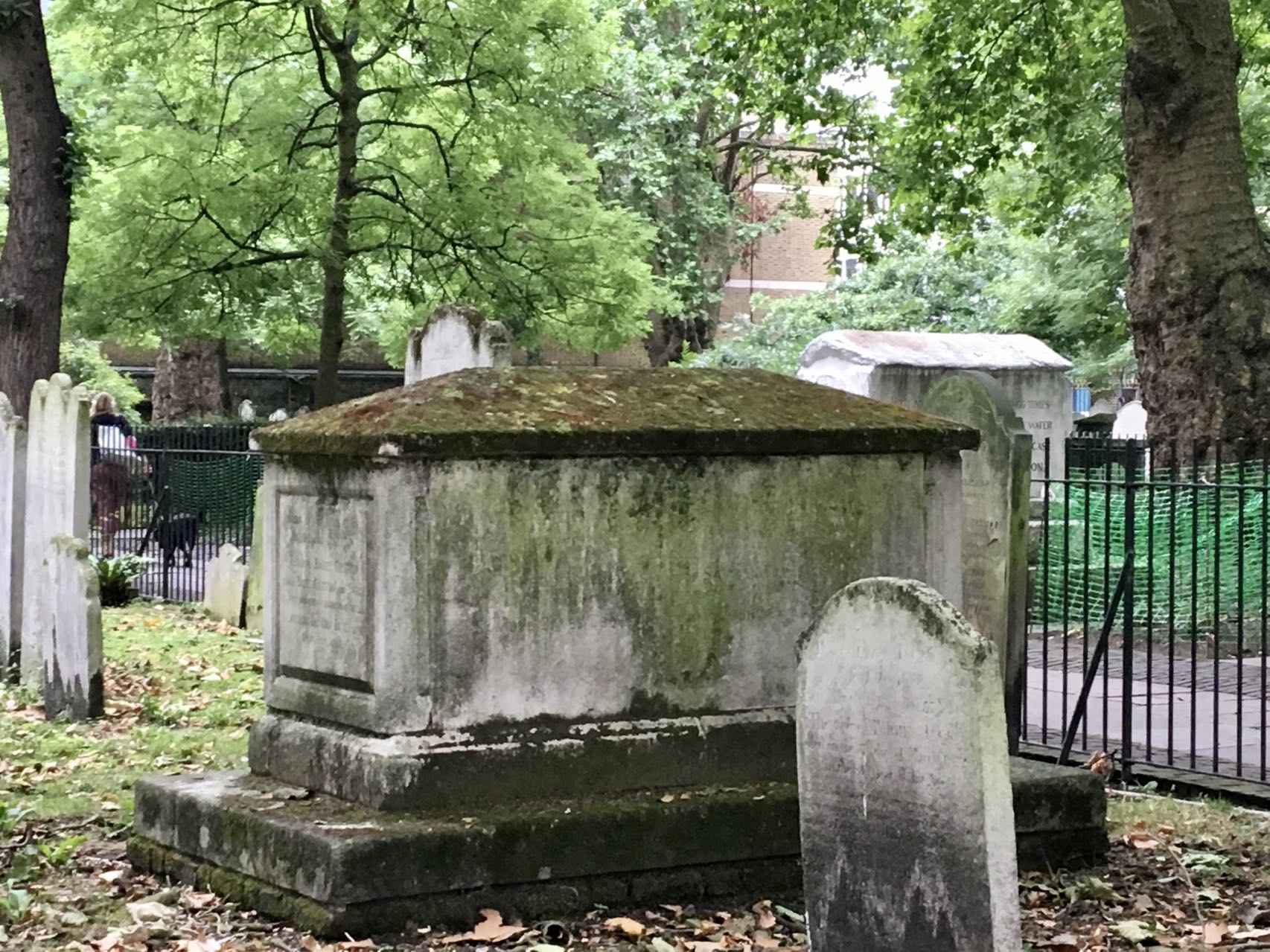
grave of reverend bayes
which i took in london circa 2017
only wife's name was engraved

thank me later...
visualize bayes
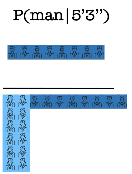
a short ghost: when walking through a naval cemetery, you saw a ghost no taller than 5'4''

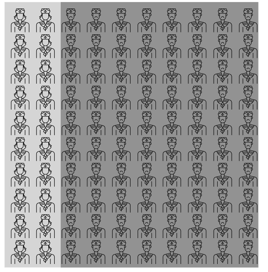
was that a biologically male or female naval officer when alive?
P(F) = 0.2
priors
P(M) = 0.8
visualize bayes
a short ghost: when walking through a naval cemetery, you saw a ghost no taller than 5'4''
was that a biologically male or female naval officer when alive?
P(F) = 0.2
likelihoods
P(M) = 0.8
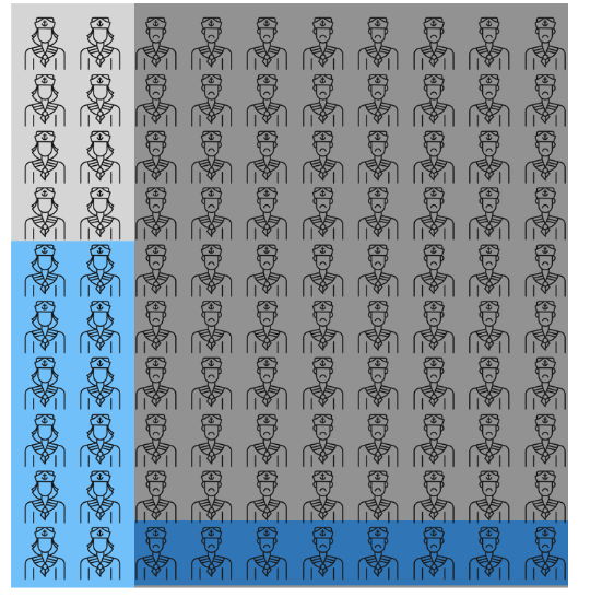
P(\leq 5'4''|F) = 0.6
P(\leq 5'4''|M) = 0.1
gray areas: impossible
visualize bayes
a short ghost: when walking through a naval cemetery, you saw a ghost no taller than 5'4''
was that a biologically male or female naval officer when alive?
posteriors
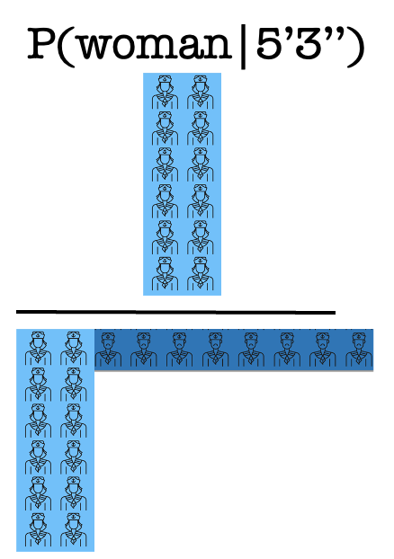
P(F|\leq 5'4'') = 0.12 / 0.2 = 0.6
marginal likelihood (sum of all unstandardized posteriors)
P(\leq 5'4''|F) \cdot P(F) + P(\leq 5'4''|M) \cdot P(M) = 0.12 + 0.08 = 0.2
P(\leq 5'4''|F) \cdot P(F) = 0.6 \times 0.2 = 0.12
unstandardized posteriors (don't sum to one)
P(\leq 5'4''|M) \cdot P(M) = 0.1 \times 0.8 = 0.08
P(M|\leq 5'4'') = 0.08 / 0.2 = 0.4
= unstandardized posteriors (prior × likelihood) / marginal likelihood
hmm...
bayesian workflow: guessing game
- host randomly picks a rule that generates numbers from 1 to 100
- H1: integers
- H2: odd numbers
- H3: even numbers
- H4: 1 to 17 (range-based)
- they give you 3 positive examples generated by this rule: [2, 4, 6]
- if you say a new number that can be generated by the rule, you win!
what would you say?
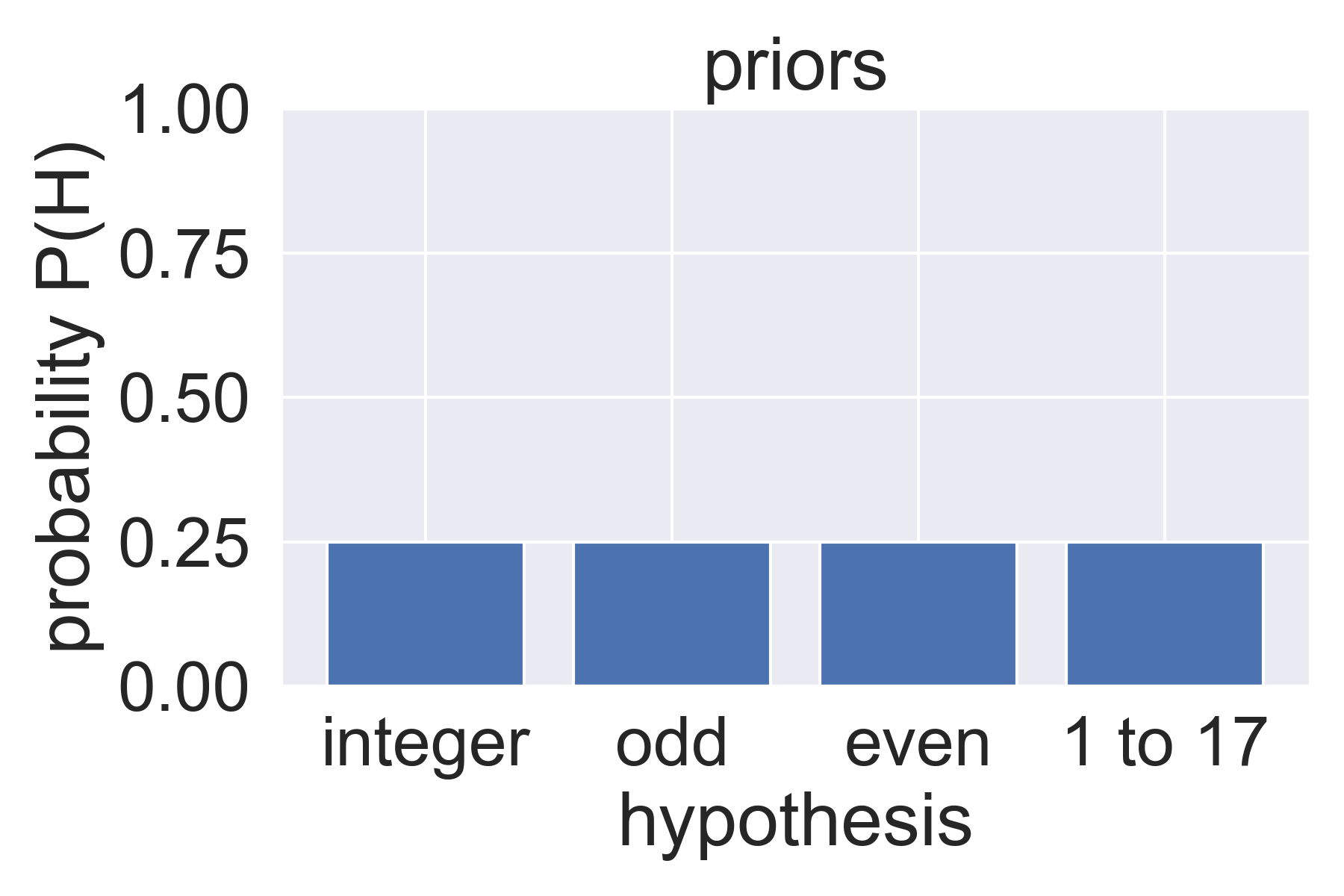
step 1: find priors 👉 probability of each hypothesis before seeing data
bayesian workflow: guessing game
step 2: prior predictive check 👉 probability of seeing each number based on priors (if you prior predictives don't generate reasonable data, rethink you priors!)
"pseudocode" (pretend python doesn't have feelings)
prior_preds = []
# loop over numbers 1-100 (NumPy array)
for number in numbers:
  # initialize each number's prior predictive at 0
  prior_pred = 0
  # loop over hypotheses
  for H, prior in zip(Hs, priors):
    # add likelihood of being accepted * prior
    if number in H:
      prior_pred += prior
  prior_preds.append(prior_pred)

why prior predictive checks?
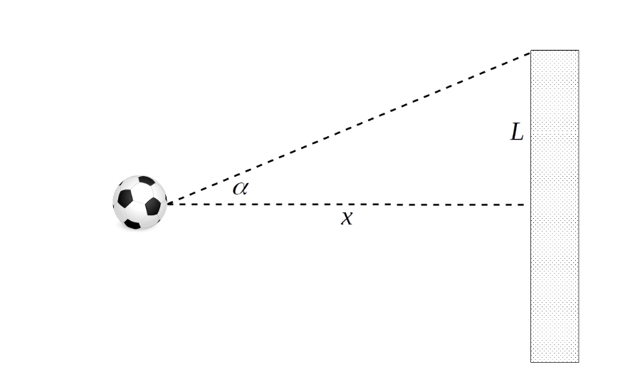
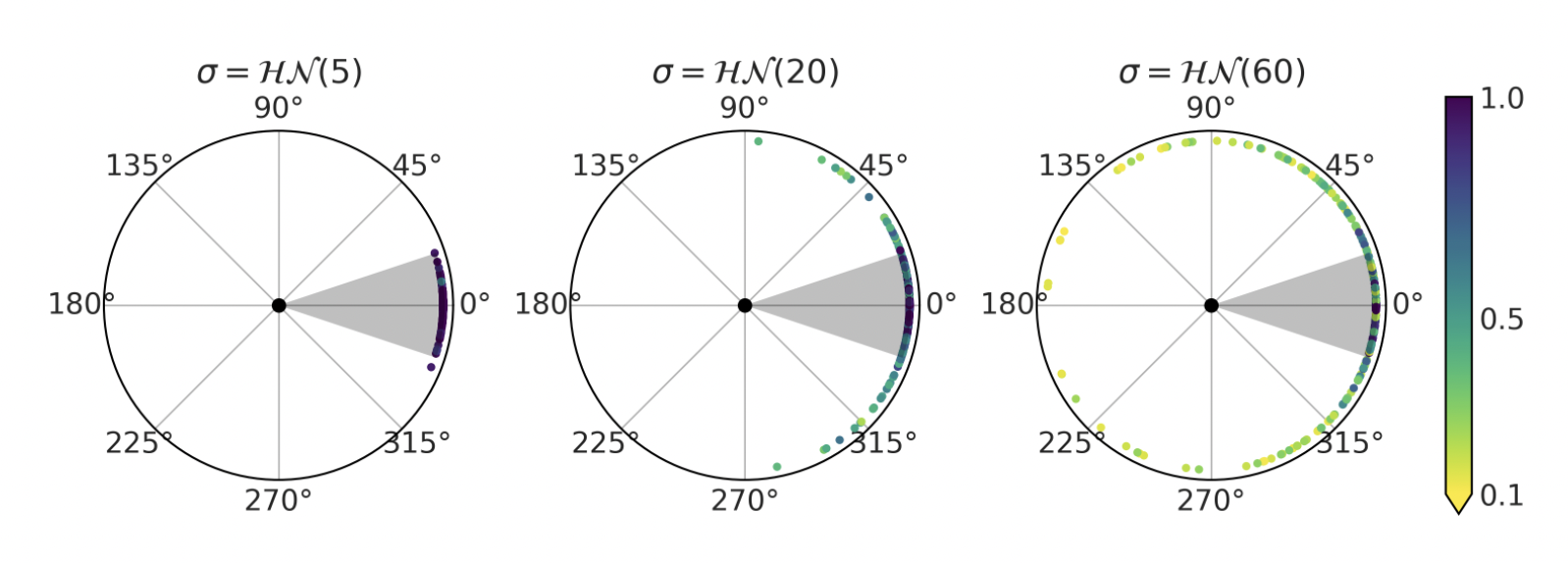
priors: probability distribution of the angle α at which the player kicks the ball
domain experts may not understand, so it's hard for them to check your assumptions
prior predictive probabilities: places where the ball can possibly land, based on your priors
a soccer player or expert can look at the graph and tell you if it looks reasonable or ridiculous
bayesian workflow: guessing game
step 3: get likelihoods 👉 probability of seeing data given a hypothesis
P(2,4,6 | H) = P(2|H) \cdot P(4|H)\cdot P(6|H)
- property of bayesian inference: if doesn't matter if you see all numbers at once, one by one, or in what order... the posteriors will be the same
-
size-principle likelihood: P(number | H)
- if a number is not in H, then H is impossible 👉 do you even need to check other numbers?
- if a number is in H, likelihood is 1 / len(H)
- likelihood of an array: product of all P(number | H)
bayesian workflow: guessing game
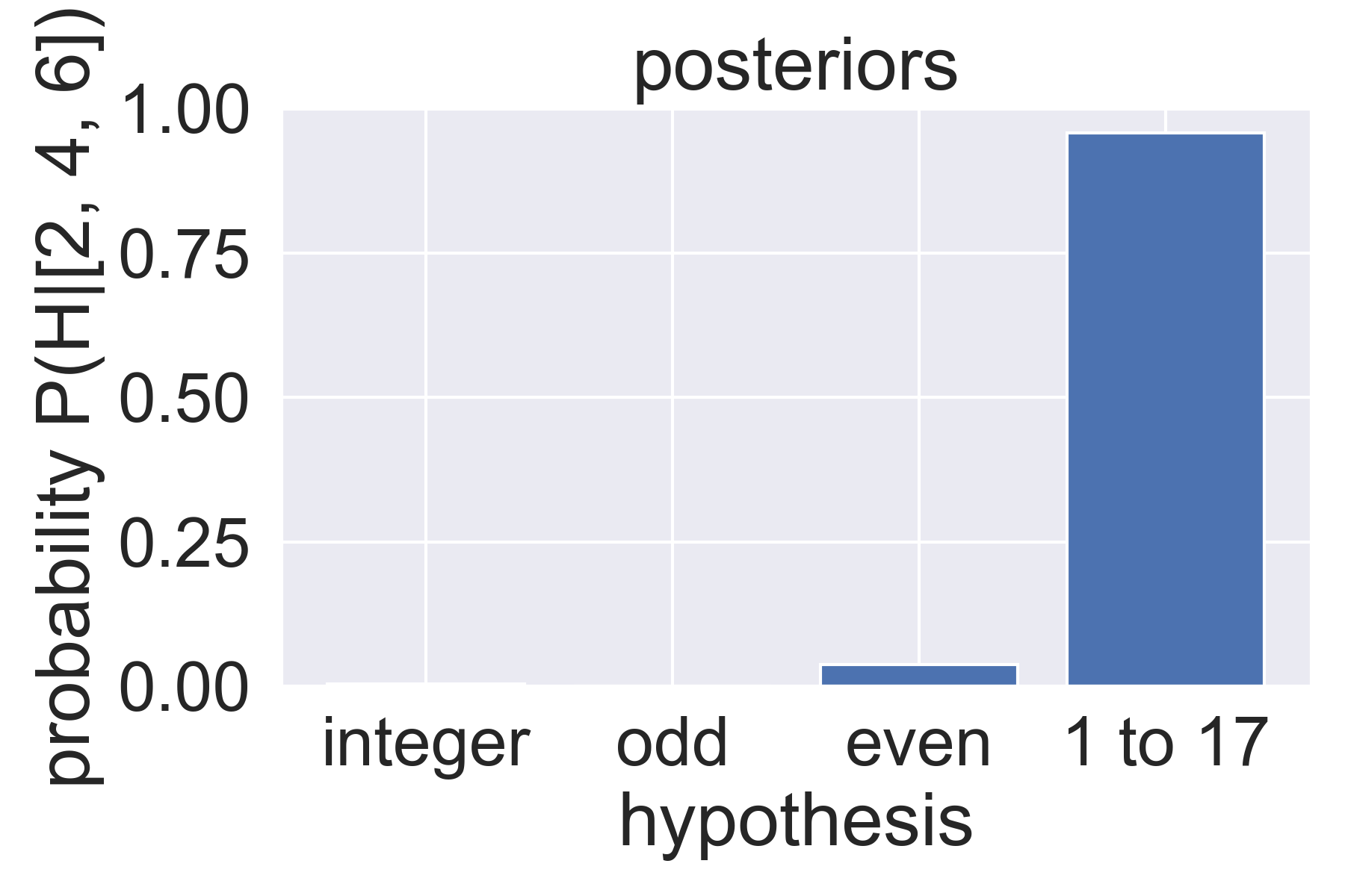
step 4: compute posteriors 👉 probability of each hypothesis after seeing data
posteriors = np.empty(len(Hs))
# loop over hypotheses
for (i, H), prior in zip(enumerate(Hs), priors):
  # unstandardized posterior
  unstandardized = get_likelihood(H, data) * prior
  posteriors[i] = unstandardized
# standardized posteriors
posteriors = posteriors / posteriors.sum()
"pseudocode"
- compute unstandardized posterior of each H: likelihood given data × prior
- standardize posteriors: divide each of the above by the sum of the above
bayesian workflow: guessing game
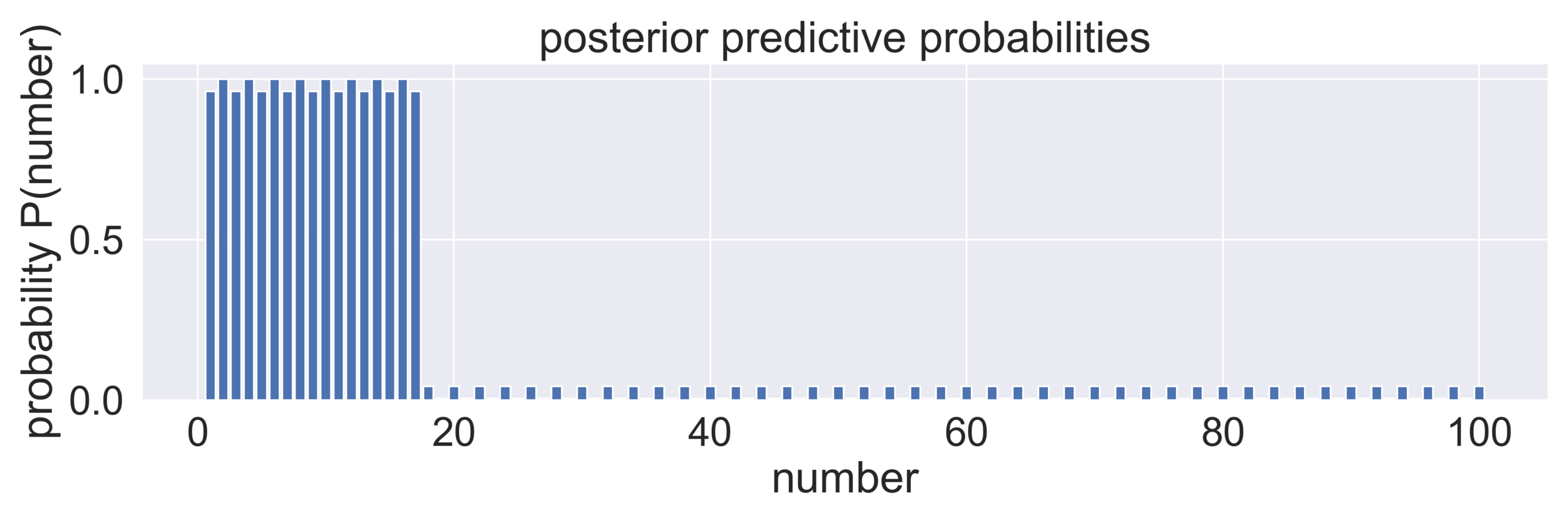
step 5: posterior predictive check 👉 probability of seeing each number based on posteriors (if your posterior predictives don't look like actual data, debug your inference)
"pseudocode": use posteriors this time (do you need different functions?)
post_preds = []
# loop over numbers 1-100 (NumPy array)
for number in numbers:
  # initialize each number's posterior predictive at 0
  post_pred = 0
  # loop over hypotheses
  for H, posterior in zip(Hs, posteriors):
    # add likelihood of being accepted * posterior
    if number in H:
      post_pred +=  post
  post_preds.append(post_pred)
hw8 prompts
range-based hypotheses: numbers from x to y, where 1 ≤ x < y ≤ 100 👉 should be many‼️
how people actually use bayes now
- exact bayesian inference is expensive 👉 marginal likelihood is a nightmare when you have many hypotheses
-
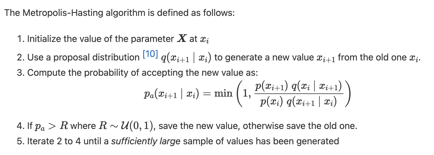
approximate inference
- markov chain monte carlo (mcmc): sample from the posterior distribution
- variational inference: use simpler distribution to approximate more complex one
in practice, you rarely wanna write your own sampler but use probabilistic programming languages such as pymc and stan (best python bayesian book)
# e.g., see coin flips (Y = HTTHH) -> infer true theta = P(H)
for iter in range(n_iters):
    # generate new theta from proposal distribution
    theta_new = stats.norm(theta, prop_sd).rvs(1)
    # compute posterior probability of new theta
    p_new = posterior(theta_new, Y, alpha, beta)
    # get ratio of new to old posterior
    ratio = p_new / p

    # accept: ratio >= cutoff (certainly) or ratio < cutoff (probabilistically)
    if ratio > stats.uniform(0, 1).rvs(1):
        theta = theta_new
        p = p_new

    # collect theta from each iteration
    trace["theta"][iter] = theta
e.g., metropolis-hastings algorithm
mcmc vs. gradient descent: the latter moves data downhill and the former collects "marbles" from the hill
cogsci131_04_04
By Yuan Meng


