Encoding a qubit into a cavity mode in circuit QED using phase estimation
Presented by Zhi Han
B. M. Terhal and D. Weigand, Encoding a Qubit into a Cavity Mode in Circuit QED Using Phase Estimation, Phys. Rev. A 93, 012315 (2016).
Overview
- GKP state
- Phase Estimation
- Implimentation
\hbar = 1
Displacement operator
The displacement operator is a common operation in optics. Since momentum is the generator of translations,
\hat D_q(a) |x\rangle:= e^{-i a \hat p}|x\rangle = |x + a\rangle
x
\(\psi (x)\)
\(e^{-ia\hat p}\psi (x)\)
GKP state: 0 and 1
|0\rangle \propto \sum_{n=-\infty}^{\infty} |2n\sqrt{\pi}\rangle_q
The \(|0\rangle\) and \(|1\rangle\) GKP states are defined to be
|1\rangle \propto \sum_{n=-\infty}^{\infty} |(2n+1)\sqrt{\pi}\rangle_q
\(|0\rangle\) and \(|1\rangle\) GKP states.
q
\(|2n\rangle\)
\(|2n+1\rangle\)
0
\(\sqrt \pi\)
\(2\sqrt \pi\)
\(3\sqrt \pi\)
\(4\sqrt \pi\)
\(5\sqrt \pi\)
\(6\sqrt \pi\)
X = e^{-i \sqrt \pi \hat p}
GKP state: technical definition
GKP state is defined to be the +1 eigenspace of \(S_q, S_p\) where
\hat S_p = e^{-i 2\sqrt{\pi} \hat p}\\
\hat S_q = e^{i 2\sqrt{\pi}\hat q}
Set the eigenvalue to be \(S_q, S_p = +1\). By definition, this implies \(|\psi\rangle\) is \(2 \sqrt \pi\) periodic.
e^{-i a \hat p}|q\rangle_q = |q + a \rangle_q
S_p|\psi\rangle_q = e^{-i 2\sqrt{\pi} \hat p}|\psi\rangle_q=|\psi\rangle_q
GKP state: + and -
|0\rangle \propto \sum_{n=-\infty}^{\infty} |2n\sqrt{\pi}\rangle_q
|1\rangle \propto \sum_{n=-\infty}^{\infty} |(2n+1)\sqrt{\pi}\rangle_q
|+\rangle=\frac{1}{\sqrt{2}}(|0\rangle+|1\rangle)
|-\rangle=\frac{1}{\sqrt{2}}(|0\rangle-|1\rangle)
|+\rangle \propto \sum_{n=-\infty}^{\infty} |n\sqrt{\pi}\rangle_q
|-\rangle \propto \sum_{n=-\infty}^{\infty} (-1)^n|n\sqrt{\pi}\rangle_q
\((-1)^n|n\rangle\)
\(|n\rangle\)
\(|+\rangle\) and \(|-\rangle\) GKP states.
q
0
\(\sqrt \pi\)
\(2\sqrt \pi\)
\(3\sqrt \pi\)
\(4\sqrt \pi\)
\(5\sqrt \pi\)
\(6\sqrt \pi\)
Z = e^{i \sqrt \pi \hat q}
\(|0\rangle\) and \(|1\rangle\) GKP states.
q
\(|2n\rangle\)
\(|2n+1\rangle\)
0
\(\sqrt \pi\)
\(2\sqrt \pi\)
\(3\sqrt \pi\)
\(4\sqrt \pi\)
\(5\sqrt \pi\)
\(6\sqrt \pi\)
\((-1)^n|n\rangle\)
\(|n\rangle\)
\(|+\rangle\) and \(|-\rangle\) GKP states.
q
0
\(\sqrt \pi\)
\(2\sqrt \pi\)
\(3\sqrt \pi\)
\(4\sqrt \pi\)
\(5\sqrt \pi\)
\(6\sqrt \pi\)
|0\rangle \propto \sum_{n=-\infty}^{\infty} |2n\sqrt{\pi}\rangle_q
|1\rangle \propto \sum_{n=-\infty}^{\infty} |(2n+1)\sqrt{\pi}\rangle_q
|+\rangle \propto \sum_{n=-\infty}^{\infty} |n\sqrt{\pi}\rangle_q
|-\rangle \propto \sum_{n=-\infty}^{\infty} (-1)^n|n\sqrt{\pi}\rangle_q
|+\rangle \propto \sum_{n=-\infty}^{\infty} |2n\sqrt{\pi}\rangle_p
|-\rangle \propto \sum_{n=-\infty}^{\infty} |(2n+1)\sqrt{\pi}\rangle_p
|0\rangle \propto \sum_{n=-\infty}^{\infty} |n\sqrt{\pi}\rangle_p
|1\rangle \propto \sum_{n=-\infty}^{\infty} (-1)^n|n\sqrt{\pi}\rangle_p
q basis
p basis
In a similar fashion, we can get the GKP states in the momentum basis instead of the position basis by taking the fourier transform.
\(|0\rangle\) and \(|1\rangle\) GKP states.
\(|+\rangle\) and \(|-\rangle\) GKP states.
q
0
\(\sqrt \pi\)
\(2\sqrt \pi\)
\(3\sqrt \pi\)
\(4\sqrt \pi\)
\(5\sqrt \pi\)
\(6\sqrt \pi\)
\((-1)^n|n\rangle\)
\(|n\rangle\)
p
\(|2n\rangle\)
\(|2n+1\rangle\)
0
\(\sqrt \pi\)
\(2\sqrt \pi\)
\(3\sqrt \pi\)
\(4\sqrt \pi\)
\(5\sqrt \pi\)
\(6\sqrt \pi\)
\((-1)^n|n\rangle\)
\(|n\rangle\)
p
0
\(\sqrt \pi\)
\(2\sqrt \pi\)
\(3\sqrt \pi\)
\(4\sqrt \pi\)
\(5\sqrt \pi\)
\(6\sqrt \pi\)
q
0
\(\sqrt \pi\)
\(2\sqrt \pi\)
\(3\sqrt \pi\)
\(4\sqrt \pi\)
\(5\sqrt \pi\)
\(6\sqrt \pi\)
\(|2n\rangle\)
\(|2n+1\rangle\)
|0\rangle \propto \sum_{n=-\infty}^{\infty} |2n\sqrt{\pi}\rangle_q
|1\rangle \propto \sum_{n=-\infty}^{\infty} |(2n+1)\sqrt{\pi}\rangle_q
X = e^{-i \sqrt \pi \hat p}
Z = e^{i \sqrt \pi \hat q}
|+\rangle \propto \sum_{n=-\infty}^{\infty} |2n\sqrt{\pi}\rangle_p
|-\rangle \propto \sum_{n=-\infty}^{\infty} |(2n+1)\sqrt{\pi}\rangle_p
X^2 = S_p = e^{-i 2 \sqrt {\pi} \hat p}
Z^2 = S_q = e^{i 2 \sqrt {\pi} \hat q}
X and Z gate
S_p = e^{-i 2 \sqrt {\pi} \hat p}
S_q = e^{i 2 \sqrt {\pi} \hat q}
Bonus: why \(2\sqrt \pi\)?
e^A e^B = e^B e^A e^{[A, B]}
S_q S_p = e^{i 2 \sqrt {\pi} \hat q} e^{-i 2 \sqrt {\pi} \hat p} = e^{-i 2 \sqrt {\pi} \hat p} e^{i 2 \sqrt {\pi} \hat q} \underbrace{e^{i 4 \pi}}_{=1} = S_p S_q
QEC with GKP states
Imagine a shift error has a occured where the state has been displaced by \(e^{-i \mu_q \hat p}\).
How can we detect and correct this error?
S_q e^{-i \mu_q \hat p } |\psi\rangle =e^{i 2\sqrt{\pi} \hat q} e^{-i \mu_q \hat p } |\psi\rangle
= e^{-i \mu_q \hat p } e^{i 2\sqrt{\pi} \hat q} e^{i 2 \sqrt \pi \mu_q}|\psi\rangle
=e^{i 2 \sqrt \pi \mu_q} e^{-i v \hat p } |\psi\rangle
S_q |\psi'\rangle = e^{i 2 \sqrt \pi \mu_q} |\psi'\rangle
q
\(|2n+\mu_q\rangle\)
0
\(\sqrt \pi\)
\(2\sqrt \pi\)
\(3\sqrt \pi\)
\(4\sqrt \pi\)
\(5\sqrt \pi\)
\(6\sqrt \pi\)
\(\mu_q\)
\(|2n\rangle\)
S_p = e^{-i 2 \sqrt {\pi} \hat p}
S_q = e^{i 2 \sqrt {\pi} \hat q}
|0\rangle \propto \sum_{n=-\infty}^{\infty} |2n\sqrt{\pi}\rangle_q
|1\rangle \propto \sum_{n=-\infty}^{\infty} |(2n+1)\sqrt{\pi}\rangle_q
\hat X = e^{-i \sqrt \pi \hat p}
\hat Z = e^{i \sqrt \pi \hat q}
Gates
Stabilizers
States
Finitely squeezed GKP states
Problem: The infinitely squeezed GKP state is not normalizable.
Idea: Replace each Dirac delta with a squeezed Gaussian state. Normalize the entire state with a Gaussian envelope.
(Terhal and Weigand 2016)
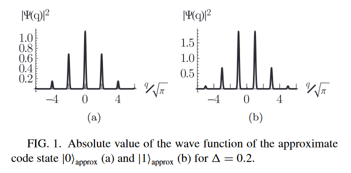
\left|\operatorname{vac}_{\mathrm{sq}}\right\rangle=\int \frac{d q}{\left(\pi \Delta^{2}\right)^{1 / 4}} e^{-q^{2} /\left(2 \Delta^{2}\right)}|q\rangle
|0\rangle_{\mathrm{approx}} \propto \sum_{t=-\infty}^{\infty} e^{-2 \pi \tilde{\Delta}^{2} t^{2}} D(t \sqrt{2 \pi})\left|\mathrm{vac}_{\mathrm{sq}}\right\rangle
=\sum_{t=-\infty}^{\infty} \int e^{-2 \pi \tilde{\Delta}^{2} t^{2}} e^{-(q-2 t \sqrt{\pi})^{2} /\left(2 \Delta^{2}\right)}|q\rangle d q,
\( \Delta = \) stdev/squeezing of mini peak
\(\tilde{\Delta} = \) stdev/squeezing of entire state
In the \(|+\rangle\) GKP state, roles of \(\tilde{\Delta}, \Delta\) are interchanged.
Rest of the talk: \(\Delta = \tilde{\Delta}\)
Infinite squeezing: \(\Delta \to 0\)
Phase Estimation
\hat U |\psi\rangle = e^{i \theta} |\psi \rangle
Measuring the complex eigenvalue \(e^{i\theta}\) of a unitary operator \(U\) is called phase estimation.
Phase Estimation, standard
control
target
Image: Quskit
Phase Estimation
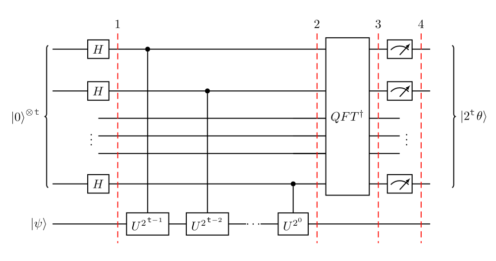
Input:
First register (control): \(n\) qubits to store the value \(2^n \theta\)
Second register (target): \(|\psi\rangle\), an eigenvector of \(U\)
- For this section we will take \(U|\psi\rangle=e^{2 \pi i \theta}|\psi\rangle\).
Step 1: Hadamard the first register. \(\left|\psi_{1}\right\rangle=\frac{1}{2^{\frac{n}{2}}}(|0\rangle+|1\rangle)^{\otimes n}|\psi\rangle\)
Step 1: Hadamard the first register. \(\left|\psi_{1}\right\rangle=\frac{1}{2^{\frac{n}{2}}}(|0\rangle+|1\rangle)^{\otimes n}|\psi\rangle\)
Phase Estimation
Step 2: Apply controlled-\(U\) gates.
- The first qubit applies \(U\) once.
- The second qubit applies \(U\) twice.
- The third qubit applies \(U\) four times.
U^{2^{j}}|\psi\rangle=U^{2^{j}-1} U|\psi\rangle=U^{2^{j}-1} e^{2 \pi i \theta}|\psi\rangle=\cdots=e^{2 \pi i 2^{j} \theta}|\psi\rangle
Since \(U|\psi\rangle=e^{2 \pi i \theta}|\psi\rangle\), the action of \(2^j\) gates corresponding to the \(j\)th qubit is:
U^{2^{j}}|\psi\rangle=U^{2^{j}-1} U|\psi\rangle=U^{2^{j}-1} e^{2 \pi i \theta}|\psi\rangle=\cdots=e^{2 \pi i 2^{j} \theta}|\psi\rangle
Phase Estimation, standard
Step 2: Apply controlled unitary gates. Using the identity
U^{2^{j}}|\psi\rangle=U^{2^{j}-1} U|\psi\rangle=U^{2^{j}-1} e^{2 \pi i \theta}|\psi\rangle=\cdots=e^{2 \pi i 2^{j} \theta}|\psi\rangle
|0\rangle \otimes|\psi\rangle+|1\rangle \otimes e^{2 \pi i \theta}|\psi\rangle=\left(|0\rangle+e^{2 \pi i \theta}|1\rangle\right) \otimes|\psi\rangle
\begin{aligned}
\left|\psi_{2}\right\rangle &=\frac{1}{2^{\frac{n}{2}}}\left(|0\rangle+e^{2 \pi i \theta 2^{n-1}}|1\rangle\right) \otimes \cdots \otimes\left(|0\rangle+e^{2 \pi i \theta 2^{1}}|1\rangle\right) \otimes\left(|0\rangle+e^{2 \pi i \theta 2^{0}}|1\rangle\right) \otimes|\psi\rangle \\
&=\frac{1}{2^{\frac{n}{2}}} \sum_{k=0}^{2^{n}-1} e^{2 \pi i \theta k}|k\rangle \otimes|\psi\rangle
\end{aligned}
\(k = \) the integer that represents a 2^n bit string. e.g. 3 = 11
Step 3: Apply inverse quantum fourier transform.
\begin{aligned}
\left|\psi_{2}\right\rangle &=\frac{1}{2^{\frac{n}{2}}}\left(|0\rangle+e^{2 \pi i \theta 2^{n-1}}|1\rangle\right) \otimes \cdots \otimes\left(|0\rangle+e^{2 \pi i \theta 2^{1}}|1\rangle\right) \otimes\left(|0\rangle+e^{2 \pi i \theta 2^{0}}|1\rangle\right) \otimes|\psi\rangle \\
&=\frac{1}{2^{\frac{n}{2}}} \sum_{k=0}^{2^{n}-1} e^{2 \pi i \theta k}|k\rangle \otimes|\psi\rangle
\end{aligned}
Q F T|x\rangle=\frac{1}{2^{\frac{n}{2}}}\left(|0\rangle+e^{\frac{2 \pi i}{2} x}|1\rangle\right) \otimes\left(|0\rangle+e^{\frac{2 \pi i}{2^{2}} x}|1\rangle\right) \otimes \ldots \otimes\left(|0\rangle+e^{\frac{2 \pi i}{2^{n-1}} x}|1\rangle\right) \otimes\left(|0\rangle+e^{\frac{2 \pi i}{2^{n}} x}|1\rangle\right)
Step 4: Measure. Obtain an integer \(2^n \theta\).
\left|\psi_{4}\right\rangle=\left|2^{n} \theta\right\rangle \otimes|\psi\rangle
For this problem, \(x = 2^n \theta\).
Standard phase estimation with a hybrid setup.
Limitations:
- Requires high number of photons
- Difficulty with controlled \(U^{2^n}\)
control
target
(Terhal and Weigand 2016)
Main idea of the paper
\hat U |\varphi\rangle \to e^{i \theta} |\psi \rangle
If we perform phase estimation on a unitary operator \(\hat U\) with an arbitrary state \(|\varphi\rangle\). Does the state go to the eigenvector \(|\psi\rangle\)? If so, can we use phase estimation to generate exotic states such as the GKP state?
\hat H |\varphi\rangle \to E |\psi \rangle
When I measure a arbitrary state \(|\varphi\rangle\) with an hermitian operator \(\hat H\), the state goes to the eigenvector \(|\psi\rangle\).
For the rest of this talk, I will refer to \[U = S_p = e^{-i 2\sqrt{\pi} \hat p}\]
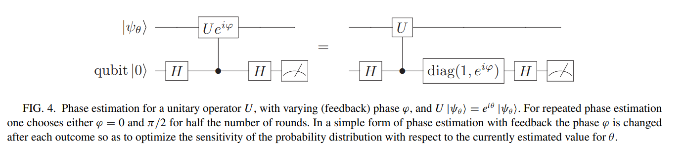
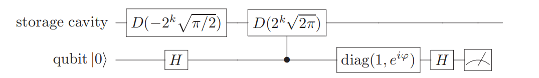
Phase estimation with repetition
control
target
(Terhal and Weigand 2016)
\hat I \otimes |0\rangle\langle 0| + \hat U \otimes |1\rangle \langle 1|
\text{diag}(1, e^{i\varphi}) = \begin{bmatrix}
1 & 0 \\
0 & e^{i\varphi}
\end{bmatrix}
Controlled-\(U\):
Diag:
|\psi\rangle \otimes |0\rangle+ e^{i \theta}|\psi\rangle\otimes |1\rangle = |\psi\rangle \otimes \left(|0\rangle+e^{i \theta}|1\rangle\right)
control
target
\langle +| \left(|0\rangle+e^{i \theta}|1\rangle\right) = \frac{1}{2}(1 + \cos(\theta)) = \text{Pr}(+|\theta)
Consider \(\varphi = 0\). On the control qubit, measure in \(|+\rangle\) basis.
\langle +| \left(|0\rangle+e^{i (\theta + \varphi)}|1\rangle\right) = \frac{1}{2}(1 - \sin(\theta)) = \text{Pr}(+|\theta)
Consider \(\varphi = \pi/2\). On the control qubit, measure in \(|+\rangle\) basis.
\frac{1}{2}(1 - \sin(\theta)) = \text{Pr}(+|\theta)_{\varphi=\pi/2}
\frac{1}{2}(1 + \cos(\theta)) = \text{Pr}(+|\theta)_{\varphi = 0}
Can be obtained experimentally
Enough to resolve ambiguity in theta
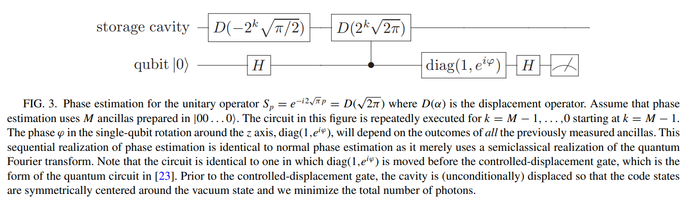
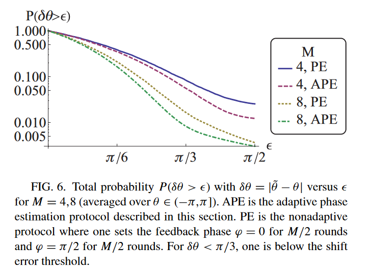
Adaptive Phase estimation
control
target
\frac{1}{2}(1 + \cos(\theta + \varphi)) = \text{Pr}_{\varphi}(+|\theta)
Idea: Optimize \(\varphi\) to gain the most information possible about \(\theta\) by considering the derivative \(\frac{\text{Pr}_{\varphi}(+|\theta)}{d\theta}\).
\frac{}{}
(Terhal and Weigand 2016)
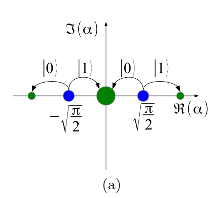
|\alpha\rangle \rightarrow|\alpha-\sqrt{\pi / 2}\rangle+(-1)^{x} e^{i \varphi}|\alpha+\sqrt{\pi / 2}\rangle
Consider a coherent state, which is not a eigenstate of
\(U = S_p\). After one round of phase estimation (with repetition), \(x = 0, 1\)
This will create a sequence of coherent states on a line. The filter is Binomial, and approximately Gaussian.
(Terhal and Weigand 2016)
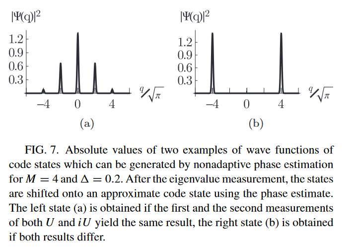
(Terhal and Weigand 2016)
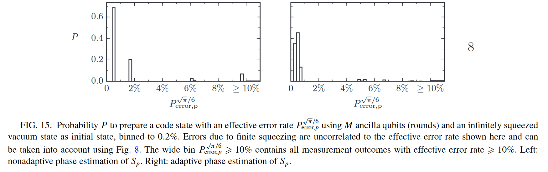
M
(Terhal and Weigand 2016)
(Terhal and Weigand 2016)
Why does this work?
Displaced GKP states
\begin{aligned}
\left|G K P_{0, \mu_{q}, \mu_{p}}\right\rangle&:= D_{q}\left(\mu_{q}\right) D_{p}\left(\mu_{p}\right)\left|G K P_{0}\right\rangle \\
\left|G K P_{1, \mu_{q}, \mu_{p}}\right\rangle&:=D_{q}\left(\mu_{q}\right) D_{p}\left(\mu_{p}\right)\left|G K P_{1}\right\rangle
\end{aligned}
Def. A displaced GKP state is a GKP state with two displacement operators \(D_q(\mu_q), D_p(\mu_p)\) and \(\mu_q ,\mu_p \in [0, \sqrt \pi)\).
Displaced GKP states
\begin{aligned}
\hat{S}_{q}\left|G K P_{\mu_{q}, \mu_{p}}\right\rangle &=e^{i 2 \sqrt{\pi} \mu_{q}}\left|G K P_{\mu_{q}, \mu_{p}}\right\rangle \\
\hat{S}_{p}\left|G K P_{\mu_{q}, \mu_{p}}\right\rangle &=e^{-i 2 \sqrt{\pi} \mu_{p}}\left|G K P_{\mu_{q}, \mu_{p}}\right\rangle
\end{aligned}
They are the eigenstates of the \(S_q, S_p\) operators.
q
\(|2n+\mu_q\rangle\)
0
\(\sqrt \pi\)
\(2\sqrt \pi\)
\(3\sqrt \pi\)
\(4\sqrt \pi\)
\(5\sqrt \pi\)
\(6\sqrt \pi\)
\(\mu_q\)
\(|2n\rangle\)
S_q e^{-i \mu_q \hat p } |\psi\rangle =e^{i 2\sqrt{\pi} \hat q} e^{-i \mu_q \hat p } |\psi\rangle
= e^{-i \mu_q \hat p } e^{i 2\sqrt{\pi} \hat q} e^{i 2 \sqrt \pi \mu_q}|\psi\rangle
=e^{i 2 \sqrt \pi \mu_q} e^{-i \mu_q \hat p } |\psi\rangle
S_q |\psi'\rangle = e^{i 2 \sqrt \pi \mu_q} |\psi'\rangle
If \(|\psi\rangle\) is a displaced GKP state, we can do error correction:
Could something like this hold for general \(|\psi\rangle\)?
\hat U |\varphi\rangle \to e^{i \theta} |\psi \rangle
Every CV state can be expressed as a superposition of displaced GKP states. For \(m \in \mathbb{Z}, \mu_q \in [0, \pi)\),
\begin{aligned}
|\psi_{cv}\rangle_{q} &=\frac{1}{\sqrt \pi} \int_{0}^{\sqrt \pi} \int_{0}^{\sqrt \pi} d \mu_{q} d \mu_{p} \, a_0(\mu_q, \mu_p) \left|G K P_{0, \mu_{q}, \mu_{p}}\right\rangle \\
&+\frac{1}{\sqrt \pi} \int_{0}^{\sqrt \pi} \int_{0}^{\sqrt \pi} d \mu_{q} d \mu_{p} \, a_1(\mu_q, \mu_p)\left|G K P_{1, \mu_{q}, \mu_{p}}\right\rangle
\end{aligned}
If we collapse the superposition \(\mu_q, \mu_p\) through phase estimation,
\left|\psi_{L}\right\rangle=a_{0}(\mu_q, \mu_p)\left|G K P_{0, \mu_{q}, \mu_{p}}\right\rangle+a_{1}(\mu_q, \mu_p)\left|G K P_{1, \mu_{q}, \mu_{p}}\right\rangle
\begin{aligned}
a_{0} &:=\sum_{m \text { even }}\left[\psi\left(\mu_{q}+m \alpha_{q}\right) e^{-i m \alpha_{q} \mu_{p}}\right] \\
a_{1} &:=\sum_{m \text { odd }}\left[\psi\left(\mu_{q}+m \alpha_{q}\right) e^{-i m \alpha_{q} \mu_{p}}\right]
\end{aligned}
\begin{aligned}
|\psi_{cv}\rangle_{q} &=\frac{1}{\sqrt \pi} \int_{0}^{\sqrt \pi} \int_{0}^{\sqrt \pi} d \mu_{q} d \mu_{p} \, a_0(\mu_q, \mu_p) \left|G K P_{0, \mu_{q}, \mu_{p}}\right\rangle \\
&+\frac{1}{\sqrt \pi} \int_{0}^{\sqrt \pi} \int_{0}^{\sqrt \pi} d \mu_{q} d \mu_{p} \, a_1(\mu_q, \mu_p)\left|G K P_{1, \mu_{q}, \mu_{p}}\right\rangle
\end{aligned}
This explains why the protocol in (Terhal and Weigand 2016) works so well:
- Displaced GKP states are the eigenstates of \(S_q, S_p\) operators
- Every CV state is a superposition of displaced GKP states.
- Phase estimation = collapsing the superposition.
- Example with two mode squeezing.
We can express a two mode squeezed state into the GKP basis.
- Step 1. Write the wavefunction. \(\psi(x) = \psi(m\sqrt \pi+\mu_q)\)
- Step 2. Perform phase estimation to measure all \( \mu_q, \mu_p\).
- Step 3. Obtain the remaining coefficients in the computational basis.
- Step 4. Convert the coefficients to the Bell basis.
\psi\left(q_{1}, q_{2}\right)=\frac{1}{\sqrt{\pi}} \exp \left(-\frac{1}{4}\left(e^{2 \zeta}\left(q_{1}+q_{2}\right)^{2}+e^{-2 \zeta}\left(q_{1}-q_{2}\right)^{2}\right)\right)
\begin{aligned}
|\psi_{cv}\rangle_{q} &=\frac{1}{\sqrt \pi} \int_{0}^{\sqrt \pi} \int_{0}^{\sqrt \pi} d \mu_{q} d \mu_{p} \, a_0(\mu_q, \mu_p) \left|G K P_{0, \mu_{q}, \mu_{p}}\right\rangle \\
&+\frac{1}{\sqrt \pi} \int_{0}^{\sqrt \pi} \int_{0}^{\sqrt \pi} d \mu_{q} d \mu_{p} \, a_1(\mu_q, \mu_p)\left|G K P_{1, \mu_{q}, \mu_{p}}\right\rangle
\end{aligned}
\begin{aligned}
\left|\psi_{L}\right\rangle &=a_{00}\left|G K P_{0, \mu_{q}, \mu_{p}}\right\rangle\left|G K P_{0, \mu_{q}, \mu_{p}}\right\rangle+a_{01}\left|G K P_{0, \mu_{q}, \mu_{p}}\right\rangle\left|G K P_{1, \mu_{q}, \mu_{p}}\right\rangle \\
&+a_{10}\left|G K P_{1, \mu_{q}, \mu_{p}}\right\rangle\left|G K P_{0, \mu_{q}, \mu_{p}}\right\rangle+a_{11}\left|G K P_{1, \mu_{q}, \mu_{p}}\right\rangle\left|G K P_{1, \mu_{q}, \mu_{p}}\right\rangle
\end{aligned}
\begin{aligned}
&a_{00}=\sum_{m_{1} \text { even }} \sum_{m_{2} \text { even }}\left[\psi\left(\mu_{q_{1}}+m_{1} \sqrt \pi \right) e^{-i m_{1} \sqrt \pi \mu_{p_{1}}} \psi\left(\mu_{q_{2}}+m_{2} \sqrt \pi \right) e^{-i m_{2} \sqrt \pi \mu_{p_{2}}}\right] \\
&a_{01}=\sum_{m_{1} \text { even }} \sum_{m_{2} \text { odd }}\left[\psi\left(\mu_{q_{1}}+m_{1} \sqrt \pi \right) e^{-i m_{1} \sqrt \pi \mu_{p_{1}}} \psi\left(\mu_{q_{2}}+m_{2} \sqrt \pi \right) e^{-i m_{2} \sqrt \pi \mu_{p_{2}}}\right] \\
&a_{10}=\sum_{m_{1} \text { odd }} \sum_{m_{2} \text { even }}\left[\psi\left(\mu_{q_{1}}+m_{1} \sqrt \pi \right) e^{-i m_{1} \sqrt \pi \mu_{p_{1}}} \psi\left(\mu_{q_{2}}+m_{2} \sqrt \pi \right) e^{-i m_{2} \sqrt \pi \mu_{p_{2}}}\right] \\
&a_{11}=\sum_{m_{1} \text { odd }} \sum_{m_{2} \text { odd }}\left[\psi\left(\mu_{q_{1}}+m_{1} \sqrt \pi \right) e^{-i m_{1} \sqrt \pi \mu_{p_{1}}} \psi\left(\mu_{q_{2}}+m_{2} \sqrt \pi \right) e^{-i m_{2} \sqrt \pi \mu_{p_{2}}}\right]
\end{aligned}
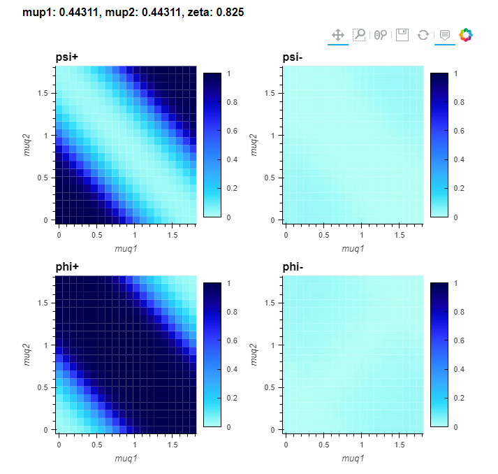
phase diagram... we find, for specific values of \(\mu_q, \mu_p \) the result is a Bell state.
Questions?
gkp
By Zhi Han


