A Little Bit of Computational Complexity
蕭梓宏
Some interesting questions
- \({\rm P \stackrel{?}{=} NP}\)
- Can we generate mathematical proofs automatically?
- Can we verify a proof looking only at very few locations of the proof?
- Does random speed up computation?
- Is approximation easier?
- How powerful is quantum computation?
Computation and Turing Machine
Turing Machine
A (k-tape) turing machine consists of:
1. k tapes that contain symbols(one of them is the input tape)
2. k read-write heads on each tape(the one on the input head is read-only)
3. a register that keeps the state of the TM
4. a finite table of instructions that given the current state and the symbols reading: write a symbol under each read/write head, move the read-write heads , and change the state
At first, the TM is in the starting state, and the input tape contains the input. Then, the TM moves according to the table of instructions until it reaches the halting state.
Turing Machine
Formally, a (k-tape) turing machine \(M\) is defined by a tuple\((\Gamma,Q,\delta)\):
\(\Gamma\) is a finite set, containing symbols that \(M\)'s tapes can contain
\(Q\) is a finite set, containing the states that \(M\) can be in
\(\delta\) is a function from \(Q \times \Gamma^k\) to \(Q \times \Gamma^{k-1} \times \{L,S,R\}^k\), and is called the "transition function"
We normally assume that \(\Gamma=\{\text{BLANK},\text{START},0,1\}\), and \(Q\) contains \(q_{start}\) and \(q_{halt}\)
Computing a function/Running TIme
Given a function \(f : \{0,1\}^* \to \{0,1\}^*\) and another function \(T: \mathbb N \to \mathbb N\),
we say a TM \(M\) computes \(f\), if for every \(x \in \{0,1\}^*\), whenever \(M\) is initialized to the start configuration on input \(x\), then it halts with \(f(x)\) written on its output tape.
We say \(M\) computes \(f\) in \(T(n)\)-time, if its computation on every input \(x\) requires at most \(T(|x|)\) steps.
Some useful facts about TM
- There exists an equivalent TM for any (C,java,...) program.(Operations in the machine language can be simulated by TMs)
- If \(f\) is computable on a k-tape TM in \(T(n)\)- time, then \(f\) is computable in time \(5kT(n)^2\) on a single-tape TM whose head movements don't depend on the input and only depends on the input length.
- Each string represents a TM, and each TM can be represented by infinitely many strings
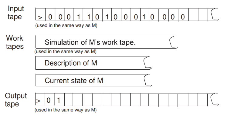
Universal TM
There exsists TM \(U\) such that for any \(x,\alpha \in \{0,1\}^*\) ,\(U(x,\alpha) = M_\alpha(x)\), where \(M_\alpha\) is the TM represented by \(\alpha\).
Moreover, if \(M_\alpha(x)\) halts within \(T\) steps then \(U(x,\alpha)\) halts within \(CT\log T\) steps, where \(C\) is independent of \(|x|\)
\(CT^2\) instead of \(CT\log T\):
Universal TM with Time Bound
There exsists TM \(U\) such that for any \(x,\alpha \in \{0,1\}^*\) , \(T \in \mathbb N\),\(U(x,\alpha,T) = M_\alpha(x)\) if \(M_\alpha(x)\) halts in \(T\) steps
Uncomputability/Undecidability?
演算法可數,問題不可勝數?
Uncomputable function
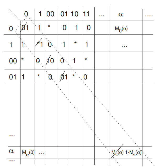
Define the function \({\rm UC}: \{0,1\}^* \to \{0,1\}\):
if \(M_\alpha(\alpha) = 1\),\({\rm UC}(\alpha) = 0\);otherwise, \({\rm UC}(\alpha) = 1\)
No turing machine can compute \(\rm UC\)!!!
Little fact: check if integer coefficient polynomial equations have integer solution is also uncomputable
Halting problem
\({\rm HALT}: \{0,1\}^* \to \{0,1\}\):
\({\rm HALT}(\langle \alpha,x \rangle) = 1\), if \(M_\alpha(x)\) halts;
\({\rm HALT}(\langle \alpha,x\rangle) = 0\), otherwise
\({\rm HALT}\) is uncomputable. WHY?
\({\rm HALT}: \{0,1\}^* \to \{0,1\}\):
\({\rm HALT}(\langle \alpha,x \rangle) = 1\), if \(M_\alpha(x)\) halts;
\({\rm HALT}(\alpha) = 0\), otherwise
If we have \(M_{\rm halt}\), then we can construct \(M_{\rm UC}\):
1. Run \(M_{\rm halt}(\alpha,\alpha)\) to see if \(M_\alpha(\alpha)\) halts
2. If it does, run \(U(\alpha,\alpha)\) to get its output
3. Ouput \(0\) if \(M_\alpha(\alpha)\) halts and outputs \(1\); output \(1\) otherwise
We can REDUCE(\(\infty \star\)) \({\rm UC}\) to \({\rm HALT}\)!
\({\rm UC}: \{0,1\}^* \to \{0,1\}\):
\({\rm UC}(\alpha) = 0\), if \(M_\alpha(\alpha) = 1\);
\({\rm UC}(\alpha) = 1\), otherwise
Uncomputability and
Gödel's Imcompleteness Theorem?
Gödel's Imcompleteness Theorem
First Incompleteness Theorem: "任何可以表達算術且一致的形式系統一定是不完備的。"
一致(consistent): There is no statement \(\phi\) such that both \(\phi\) and \(\neg \phi\) can be proven
完備(complete): For every statement \(\phi\), either \(\phi\) or \(\neg \phi\) can be proven
Gödel's Imcompleteness Theorem
There are true statements that cannot be proven!
(in certain axiomatic systems, like ZFC)
For example, the consistency of ZFC cannot be proven in ZFC.
Gödel's imcompleteness theorem motivated Church and Turing into their work on uncomputability.
The other way?
From Halting Problem to
Incompleteness Thorem
Weaker version of First Incompleteness Theorem: "任何可以表達算術且可靠的形式系統一定是不完備的。"
可靠(sound): If a statement \(\phi\) is not true, it cannot be proven(which implies consistent)
完備(complete): For every statement \(\phi\), either \(\phi\) or \(\neg \phi\) can be proven
From Halting Problem to
Incompleteness Thorem
If a axiomatic system(that is powerful enough) is both sound and complete , we can devise an algorithm(or, a TM) that can compute \(\rm HALT\)!
From Halting Problem to
Incompleteness Thorem
step 0: Read the input \(\alpha\) and \(x\)
step 1: Express the statement "\(M_\alpha\) halts on \(x\)" by \(\phi\)
step 2: Enumerate all strings of finite length, and check if it is a proof for \(\phi\) or \(\neg \phi\)(proof checking is not hard!)
step 3: By completeness, step 2 can find the proof, and by soundness, the proven result is true. Thus we can output \(1\) if \(\phi\) is true and output \(0\) otherwise!
Why Turing Machine?
The Church-Turing(CT) Thesis: Every effectively calculable function is a computable function
\(\lambda\)-calculus
general recursive function
Markov alogorithm
pointer machine
combinatory logic
computationally equivalent to TMs
P
Language/Decision Problem
A language \(L\) is a subset of
\(\{0,1\}^*\)(the set of all (bit)strings)
A decision problem for \(L\) is:
"Given \(x\): output 1 if \(x \in L\), else output 0"
*We can turn many objects into strings, like integers, pairs of integers, matrix, graph,...,and turing machines!
Language/Decision Problem
Examples of languages:
PAL:\(\{s:s \text{ is a palindrome}\}\)
PRIME:\(\{n: n \text{ is a prime number}\}\)
MAXINDSET:\(\{\langle G,k\rangle:\text{ the size of the largest independent set } \text{ in } G \text{ is } k\}\)
Complexity Class
A complexity class is a set of languages(boolean functions) that can be decided(computed) within given resource bounds.
DTIME and P
\({\rm DTIME}(T(n))\): a language \(L\) is in \({\rm DTIME}(T(n))\) if there is a TM that decides \(L\) in \(O(T(n))\) time
P: \(P = \cup_{c \geq 1} {\rm DTIME}(n^c)\)
We say that problems in P are efficiently solvable
Examples?
NP
NP
a language \(L\) is in \(\rm NP\) :
there exists a polynomial \(p\), a polynomial-time TM \(M\), such that \(\forall x \in \{0,1\}^*, \\ x\in L \Leftrightarrow \exists u \in \{0,1\}^{|p(|x|)|},{\rm s.t.} M(u,x)=1 \)
"A 'yes' instance can be verified in polynomial time with a certificate."
NP
Examples of languages in NP:
PAL:\(\{s:s \text{ is a palindrome}\}\)
COMPOSITE:\(\{n: n \text{ is a composite number}\}\)
SUBSETSUM:\(\{\langle A_1,A_2,...,A_n,T\rangle:\text{ there is a subset of } A \text{ that sum to } T \}\)
Are they in NP?
INDSET:\(\{\langle G,k\rangle:\text{ there is a independent set of size } k \text{ in } G \}\)
MAXINDSET:\(\{\langle G,k\rangle:\text{ the size of the largest independent set } \text{ in } G \text{ is } k\}\)
GI:\(\{\langle G,G'\rangle: G \text{ is isomorphic to } G' \}\)
GNI:\(\{\langle G,G'\rangle: G \text{ is not isomorphic to } G' \}\)
?
?
Non-Deterministic TM
An NDTM \(M\) is almost the same as a TM, but it has a special state \(q_{\rm accept}\) and two transition functions \(\delta_0\) and \(\delta_1\). In each step of computation, \(M\) arbitrarily choose one of them to apply.
For \(x\in\{0,1\}^*\), we say that \(M(x) = 1\) if there exists some sequence of these choices that makes \(M\) reach \(q_{\rm accept}\).(Otherwise, \(M(x)\) = 0)
We say that \(M\) runs in \(T(n)\) time, if for all \(x\in \{0,1\}^*\) and every sequence of choices, \(M\) reaches either \(q_{\rm halt}\) or \(q_{\rm accept}\) within \(T(|x|)\) steps.
NTIME
\({\rm NTIME}(T(n))\): a language \(L\) is in \({\rm NTIME}(T(n))\) if there is a \(O(T(n))\) NDTM \(M\), such that \(x \in L \Leftrightarrow M(x) = 1\)
Theorem 1:
\({\rm NP} = \cup_{c \geq 1} {\rm NTIME}(n^c)\)
Idea:
The choices that make the NDTM reach \(q_{\rm accept}\) can be used as the certificate(and vice versa).
Polynomial-time Reduction
A language \(L\) is polynomial-time reducible to another language \(L'\)(\(L \leq_p L'\)), if there exists a polynomial-time computable function \(f:\{0,1\}^* \to \{0,1\}^*\) such that \(x \in L \Leftrightarrow f(x) \in L'\)
\(L \leq_p L', L' \leq_p L'' \Rightarrow L \leq_p L''\)
example: we can reduce 3-coloring to 4-coloring.
NP hard and NP complete
NP-hard: \(L'\) is in NP-hard, if \(L \leq_p L'\) for every \(L\) in NP
NP-complete: \(L'\) is NP-complete if it is in NP and NP-hard
CNF(CNF formula)
a CNF instance with 5 variables and 4 clauses:
\(\phi(a_1,a_2,a_3,a_4,a_5) = (a_1\lor \neg a_2 \lor a_3 \lor a_4) \land (\neg a_1 \lor a_2 \lor a_3 \lor a_5) \land (\neg a_1 \lor \neg a_4 \lor a_5) \land (a_2 \lor \neg a_3 \lor \neg a_5)\)
a 3CNF instance with 5 variables and 4 clauses:
\(\phi(a_1,a_2,a_3,a_4,a_5) = (a_1\lor \neg a_2 \lor a_3) \land (\neg a_1 \lor a_2 \lor a_3 ) \land (\neg a_1 \lor \neg a_4 \lor a_5) \land (a_2 \lor \neg a_3 \lor \neg a_5)\)
A CNF is satisfiable if there exists some assignment of the variables such that \(\phi\) is true.
clause
literal
SAT and 3SAT
SAT:\(\{\phi: \phi \text{ is a satisfiable CNF}\}\)
3SAT:\(\{\phi: \phi \text{ is a satisfiable 3CNF}\}\)
Cook-Levin Theorem:
SAT and 3SAT is NP-complete.
We can see that SAT and 3SAT is in NP.
Our goal is to
1. reduce every \(L \in {\rm NP}\) to SAT,
2. reduce SAT to 3SAT
useful tool
Every boolean function \(f:\{0,1\}^l \to \{0,1\}\) can be expressed as a CNF with \(2^l\) clauses of \(l\) literals
\(\phi(x) = \bigwedge\limits_{z:f(z) = 0} (x \neq z)\)
| x_1 | x_2 | x_3 | f(x) |
|---|---|---|---|
| 0 | 0 | 0 | 1 |
| 0 | 0 | 1 | 0 |
| 0 | 1 | 0 | 1 |
| 0 | 1 | 1 | 0 |
| 1 | 0 | 0 | 0 |
| 1 | 0 | 1 | 1 |
| 1 | 1 | 0 | 1 |
| 1 | 1 | 1 | 1 |
\(\phi(x) = (x_1 \lor x_2 \lor \neg x_3) \land\\ (x_1 \lor \neg x_2 \lor \neg x_3)\land\\ (\neg x_1 \lor x_2 \lor x_3)\)
CL Theorem Proof
We want to reduce a language \(L\) in NP to SAT(in polynomial time).
Given \(x \in \{0,1\}^*\), we want to construct \(\phi_x\) such that
\(\phi_x \in {\rm SAT} \Leftrightarrow M(x,u) = 1 \text{ for some } u \in \{0,1\}^{p(|x|)}\)
Since \(L\) is in NP, there is a polynomial time TM \(M\) such that
\(x \in L \Leftrightarrow M(x,u)=1\) for some \(u \in \{0,1\}^{p(|x|)}\)
CL Theorem Proof
We can assume that:
\(M\) has only two tapes (input + work / output) and it is oblivious(so the location of its heads in the \(i\)-th step only depends on the input length and \(i\))
CL Theorem Proof
Snapshot:
The snapshot of the \(i\)-th step of \(M\)'s computation on input \(y = x \circ u\) is a triple \(\langle a,b,q \rangle \in \Gamma \times \Gamma \times Q\), representing the symbols on the two tapes and the state that \(M\) is in.
Encode the snapshot of the \(i\)-th step as \(z_i \in \{0,1\}^c\), where \(c\) is only dependent of \(|\Gamma|\) and \(|Q|\).
If someone claims that \(M(x,u) = 1\) and provides you the snapshot of the computation, how can you tell whether the snapshots present a valid computution by \(M\)?
CL Theorem Proof
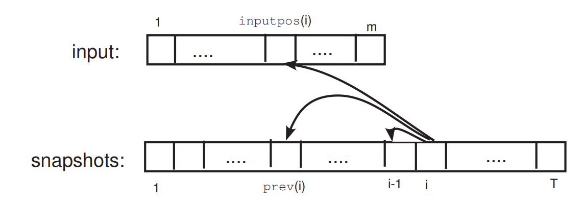
\(z_i\) depends on: the state in step \(i-1\) and the symbols in the currenct cells of the two tapes
There is a function \(F:\{0,1\}^{2c+1} \to \{0,1\}^c\), such that
\(z_i=F(z_{i-1},z_{{\rm prev}(i)},y_{{\rm inputpos}(i)})\)
\(F\) only depends on \(M\); \({\rm prev}(i)\) and \({\rm inputpos}(i)\) only depend on \(M\) and \(|y|\), and can be known by simulating \(M(0^{|y|})\).
CL Theorem Proof
Given \(x \in \{0,1\}^*\), we want to construct \(\phi_x\) such that
\(\phi_x \in {\rm SAT} \Leftrightarrow M(x,u) = 1 \text{ for some } u \in \{0,1\}^{p(|x|)}\)
\(M(x,u) = 1 \text{ for some } u \in \{0,1\}^{p(|x|)} \Leftrightarrow \)
there exist \(y \in \{0,1\}^{|x|+p(|x|)}\) and \(z \in \{0,1\}^{c(T(n)+1)}\), such that
1. The first \(n\) bits of \(y\) are equal to \(x\)
2. \(z_0\) encodes the initial snapshot of \(M\)
3. For every \(i\in [1,T(n)],z_i = F(z_{i-1},z_{{\rm prev}(i)},y_{{\rm inputpos}(i)})\)
4. \(z_{T(n)}\) encodes a snapshot in which \(M\) halts and outputs \(1\).
CL Theorem Proof
Given \(x \in \{0,1\}^*\), we want to construct \(\phi_x\) such that
\(\phi_x \in {\rm SAT} \Leftrightarrow M(x,u) = 1 \text{ for some } u \in \{0,1\}^{p(|x|)}\)
\(M(x,u) = 1 \text{ for some } u \in \{0,1\}^{p(|x|)} \Leftrightarrow \)
there exist \(y \in \{0,1\}^{|x|+p(|x|)}\) and \(z \in \{0,1\}^{c(T(n)+1)}\), such that
1. "usefull tool": \(n\) clauses of size \(4\)
2. "useful tool": \(2^c\) clauses of size \(c\)
3. "useful tool": \(T(n) 2^{3c+1}\) clauses of size \(3c+1\)
4. "useful tool": \(2^c\) clauses of size \(c\)
Just let \(\phi_x\) be the AND of the above conditions!
NP completeness of 3SAT
Now we know SAT is NP-complete, so we can show that 3SAT is NP-complete by reducing SAT to 3SAT in polynomial time.
\((a_1\lor \neg a_2 \lor a_3 \lor a_4 \lor \neg a_5) \\ \Leftrightarrow (a_1\lor \neg a_2\lor a_3 \lor b_1) \land (a_4 \lor \neg a_5 \lor \neg b_1)\)
\(\Leftrightarrow (a_1\lor \neg a_2\lor b_2) \land (a_3 \lor b_1 \lor \neg b_2) \land (a_4 \lor \neg a_5 \lor \neg b_1)\)
We can easily turn a clause of \(k\) variables into AND of \(k-2\) clauses of \(3\) variables!
Reduction 大賽
INDSET: Decide if there is a independent set of size \(k\) on \(G\)
QUADEQ: Decide if the set of boolean quadratic equations (\(\sum_{i,j \in [n]} a_{i,j}u_i u_j = b\)) is satisfiable(addition is modulo 2)
dHAMPATH: Decide if the directed graph \(G\) has a hamiltonian path
Exactly One 3SAT: Decide if there is an assigment such that in each clause of the CNF, exactly one of the literals is TRUE
TSP: Decide if there is a closed circuit that visits every node exactly once with total length at most \(k\) on a weighted complete graph \(G\)
HAMPATH: Decide if the undirected graph \(G\) has a hamiltonian path
SUBSETSUM: Decide if a subset of the sequence \(A\) sum up to \(T\)
coNP(順便講)
1. coNP = \(\{L : \bar L \in {\rm NP}\}\)
2. We say a language \(L\) is in coNP if there are a polynomial time TM \(M\) and a polynomial \(p\) such that
\(x \in L \Leftrightarrow \forall u \in \{0,1\}^{p(|x|)}, M(x,u) = 1\)
Why are the two defenitions equivalent?
example:GNI,tautology
Hardness of Approximation
MAX-3SAT
For a 3CNF \(\phi\), we denote \({\rm val}(\phi)\) as the maximum fraction of clauses that can be satisfied by any assigment.
If \(\phi\) is satisfiable, then \({\rm val}(\phi) = 1\).
\(\rho\)-approximation
For a CNF \(\phi\), can we find an assignment that satisfies \(\rho \cdot{\rm val}(\phi)\) of \(\phi's\) clauses in polynomial time?
For a graph \(G\) whose maximum independent set has size \(k\), can we find an independent set of size \(\rho \cdot k\) in polynomial time?
For a graph \(G\) whose minimum vertex cover has size \(k\), can we find an vertex cover of size \(\frac{k}{\rho}\) in polynomial time?
Can \(\rho\) be arbitrarily close to \(1\)?
PCP Theorem
PCP verifier?
Example: \({\rm GNI} \in {\rm PCP}({\rm poly}(n),1)\)(GNI has a PCP verifier that uses poly(n) random coins and \(O(1)\) queries to the proof)
Verifier(\(V\)): By tosing random coins and making queries to the proof, the verifier should accept if \(G_1\not \equiv G_2\).
Proof(\(\pi\)): The proof is a string, and is expected that for each \(n\)-vertex labeled graph \(H\), \(\pi[H] = 0\) if \(H \equiv G_0\) and \(\pi[H] = 1\) otherwise.
\(V\) flips a coin to get \(b \in \{0,1\}\) and flips \(O(n \log n)\) coins to get a random permutation \(P\) of length \(n\).
\(V\) applies \(P\) to the vertices of \(G_b\) to obtain \(H\), and accept iff \(\pi[H] = b\).
Efficient: runs in polynomial time and uses limited random coins and queries
Complete: always accepts if \(x \in L\)
Sound: accepts with probability at most \(\frac{1}{2}\) if \(x \not \in L\)
香草口味PCP theorem
\({\rm NP}={\rm PCP}(\log n,1)\)
Each language in NP has a PCP verifier that uses \(O(\log n)\) random coins and makes \(O(1)\) queries to the proof.
We can then probabilisticlly check a mathemaical proof by only examining a constant bit of the proof!
巧克力口味PCP theorem
There exists \(\rho < 1\), such that for every \(L \in \rm NP\) there is a polynomial function \(f\) mapping strings to 3CNF such that :
\(x \in L \Rightarrow {\rm val}(f(x)) = 1\)
\(x \not\in L \Rightarrow {\rm val}(f(x)) < \rho\)
Thus, there exists some \(\rho < 1\) such that if there is a \(\rho\)-approximation algortihm for MAX-3SAT, then P=NP.
Why are they equivalent?
巧克力:There exists \(\rho < 1\), such that for every \(L \in \rm NP\) there is a polynomial function \(f\) mapping strings to 3CNF such that :
\(x \in L \Rightarrow {\rm val}(f(x)) = 1\)
\(x \not\in L \Rightarrow {\rm val}(f(x)) < \rho\)
香草:Each language in NP has a PCP verifier \(V\) that uses \(O(\log n)\) random coins and makes \(O(1)\) queries to the proof.
香草到巧克力:Define \(V_{x,r} \in \{0,1\}\) as the output of \(V\) if the random coin tosses are \(r\)(\(r \in \{0,1\}^{c \log n}\)). Since \(V_{x,r}\) only depends on \(q\) bits of the proof, we can express \(V_{x,r}\) by a 3CNF with \(q2^q\) clauses(\({\rm poly}(n) \cdot q2^q\) clauses in total).
Why are they equivalent?
巧克力:There exists \(\rho < 1\), such that for every \(L \in \rm NP\) there is a polynomial function \(f\) mapping strings to 3CNF such that :
\(x \in L \Rightarrow {\rm val}(f(x)) = 1\)
\(x \not\in L \Rightarrow {\rm val}(f(x)) < \rho\)
香草:Each language in NP has a PCP verifier \(V\) that uses \(O(\log n)\) random coins and makes \(O(1)\) queries to the proof.
巧克力到香草:For an input \(x\), the verifier computes \(f(x)\) and expect the proof to be a satisfying assigment for \(f(x)\). Then the verifier just randomly choose one clause of \(f(x)\) and look at the corresponding three bits of the proof to check.
Maxmimum Independent Set and Minimum Vertex Cover
By the reduction of 3SAT to INDSET, we can transform a CNF \(\phi\) to a \(n\)-vertex graph whose largest independent set has size \({\rm val}(\phi)\frac{n}{7}\)
By the PCP theorem, if \({\rm P} \neq {\rm NP}\), there exists \(\rho < 1\) such that we cannot decide if \({\rm val}(\phi) = 1\) or \({\rm val}(\phi) < \rho\).
\({\rm val}(\phi)\)
最大獨立集
最小點覆蓋
1
\(<\rho\)
\(\frac{n}{7}\)
\(<\rho\frac{n}{7}\)
\(n-\frac{n}{7}\)
\(>n - \rho \frac{n}{7}\)
\(\frac{n-\frac{n}{7}}{n-\rho\frac{n}{7}} = \frac{6}{7-\rho}\), thus we cannot \(\rho\)-approximate the maximum independent set or \(\frac{6}{7-\rho}\) -approximate the minimum vertex cover.
Approximation of maximum independent set
In fact, we cannot \(\rho'\)-approximate the maximum independent set for any \(\rho'\)!
\(G^k\)
\(G\)
\(G^2\)
\({\rm IS}(G^k) = ({\rm IS}(G))^k\)
Maxmimum Independent Set and Minimum Vertex Cover
By the reduction of 3SAT to INDSET, we can transform a CNF \(\phi\) to a \(n\)-vertex graph whose largest independent set has size \({\rm val}(\phi)\frac{n}{7}\)
\({\rm val}(\phi)\)
\({\rm IS}(G)\)
1
\(<\rho\)
\(\frac{n}{7}\)
\(<\rho\frac{n}{7}\)
\((\frac{n}{7})^k\)
\({\rm IS}(G^k)\)
\(<\rho^k(\frac{n}{7})^k\)
For any \(\rho' > 0\), there exits \(k\) such that \(\rho^k < \rho'\), thus we cannot \(\rho'\)-approximate IS in polynomial time if \({\rm P} \neq {\rm NP}\)
Proof of the PCP theorm
沒了啦><
Reference
Sanjeev Arora and Boaz Barak(2009):Computational Complexity: A Modern Approach
Communication Complexity?
What is communication complexity?
Communication Complexity
For a function \(f(x,y)\), where \(x\in \mathcal X, y \in \mathcal Y\), we give \(x\) to Alice(A) and \(y\) to Bob(B), and they both need to know \(f(x,y)\).
A protocol is an algorithm that decide how A and B communicate. The length of a protocol is the maximum number of bits A and B need to exchange over all \((x,y)\).
The communication complexity of \(f\) is the minimum length of all protocols that "computes" \(f\).
Examples!
For \(x,y\in \{0,1\}^n\),
$$ EQ(x,y)=\left\{\begin{matrix}1 & ({\rm if}\ x=y)\\ 0 & ({\rm if}\ x\neq y)\end{matrix}\right.$$
Let \(x,y\) be lists of numbers in \([n]\) whose length is \(t\).
\(MD(x,y)\) is the median of the combination of the two lists.
* However, we usually assume \(f(x,y) \in \{0,1\}\).
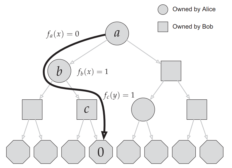
Formal Definition of Protocols
A protocol \(\pi\) can be specified by a full binary tree, where each non-leaf vertex has an owner and an associated function \(f_v: \mathcal X( {\rm or}\ \mathcal Y) \to \{0,1\}\), and each leaf has an output.
Each input \((x,y)\) induce a path from the root to the leaf \(\pi(x,y)\). We say \(\pi\) computes a function \(f\) if the output of \(\pi(x,y)\) is equal to \(f(x,y)\) for all possible inputs.
The length of the protocol is the depth of the tree.
Randomized Protocols?
In the randomized case, A and B can both see an infinitely-long sequence \(R\) of unifromly random bits(independent of their inputs), and the protocol can make errors.
We say a protocol \(\pi\) computes \(f\) with error \(\epsilon < \frac{1}{2}\), if for all \((x,y)\), $$\Pr_{R}[\pi_R(x,y) \neq f(x,y)] \leq \epsilon$$
The length of \(\pi\) is the maximum number of bits exchanged(over all \(R,x,y\)). The randomized communication complexity of \(f,\epsilon\) is the minimum length of all randomized ptotocol that computes \(f\) with error \(\epsilon\).
Examples!
For \(x,y\in \{0,1\}^n\),
$$ EQ(x,y)=\left\{\begin{matrix}1 & ({\rm if}\ x=y)\\ 0 & ({\rm if}\ x\neq y)\end{matrix}\right.$$
Some Other Problems
For \(x,y\in \{0,1\}^n\),
$$ GT(x,y)=\left\{\begin{matrix}1 & ({\rm if}\ x\geq y)\\ 0 & ({\rm if}\ x < y)\end{matrix}\right.$$
For \(x,y\in \{0,1\}^n\),
$$ DISJ(x,y)=\left\{\begin{matrix}1 & ({\rm if}\ |x \cap y|=0)\\ 0 & ({\rm otherwise})\end{matrix}\right.$$
For \(x,y\in \{0,1\}^n\),
$$ IP(x,y)=\langle x,y \rangle \% 2$$
Lower Bounds
Deterministic
Functions and Matrices
For a function \(f(x,y)\), we can represent it as a matrix \(M_f\).
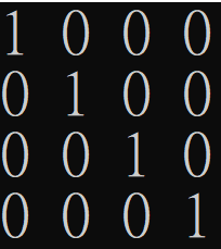
\(M_{EQ}\)(2-bit)
Rectangles
A rectangle is a subset of the input space \(\mathcal X \times \mathcal Y\) of the form \(A\times B\), where \(A\in \mathcal X, B \in \mathcal Y\).
Rectangles and Protocols
After Alice and Bob communicate according to the protocol, a rectangle is induced.
The rectangle must be monochromatic in \(M_f\).
Rectangles and Protocols
Thus, if there exists a protocol of length \(c\) for computing \(f\), then \(M_f\) can be partitioned into \(2^c\) monochromatic rectangles.
If every partition of \(M_f\) into monochromatic rectangles requires at least \(t\) rectangles, then the deterministic complexity of \(f\) is at least \(\log t\).
\(\implies\)
Rectangles and Protocols
Thus, if there exists a protocol of length \(c\) for computing \(f\), then \(M_f\) can be partitioned into \(2^c\) monochromatic rectangles.
If every cover of \(M_f\) by monochromatic rectangles requires at least \(t\) rectangles, then the deterministic complexity of \(f\) is at least \(\log t\).
(\(\infty \star\))
\(\implies\)
Rectangles and Protocols
Is the converse true?
However, if \(M_f\) can be partitioned into \(2^c\) rectangles, then there is a protocol of length \(O(c^2)\) that computes \(f\).
Deterministic Lower Bound of EQ and GT
\(M_{EQ}\)
\(M_{GT}\)
Fooling Set
A fooling set \(F \) of \(f(x,y)\) is a subset of inputs such that
1. \(f\) is constant on \(F\), and
2. for all \((x_1,y_1),(x_2,y_2) \in F\), either \((x_1,y_2) \) or \((x_2,y_1) \) has the opposite \(f-\)value
The size of the (monochromatic) rectangle cover of \(M_f\) is at least the size of \(|F|\).
The deterministic communication complexity of \(f\) is at least \(\log f\).
Deterministic Lower Bound of DISJ
For \(x,y\in \{0,1\}^n\),
$$ DISJ(x,y)=\left\{\begin{matrix}1 & ({\rm if}\ |x \cap y|=0)\\ 0 & ({\rm otherwise})\end{matrix}\right.$$
\(F = \{(x,\bar x)|x \in \{0,1\}^n\}\) is a fooling set.
The Deterministic Communication Complexity of DISJ is n+1.
Rank
The deterministic communication complexity of \(f\) is at least \(\log({\rm rank}(M_f)+1)\)
\({\rm rank}(M_f)\) is the smallest number \(r\) such that \(M_f\) can be expressed as the sum of \(r\) matrices of rank 1
Protocol of length \(c\) implies a partition of \(2^c\) rectangles.
Thus, \({\rm rank}(M_f) \leq 2^c-1\).
Lower Bounds from Rank
\(M_{EQ}\)
\(M_{GT}\)
Some Lemmas
\({\rm rank}(M\otimes M') = {\rm rank}(M) \cdot {\rm rank}(M')\)
$${\rm rank}(A) - {\rm rank}(B) \leq {\rm rank}(A+B) \leq {\rm rank}(A) + {\rm rank}(B)$$
Lower Bounds from Rank
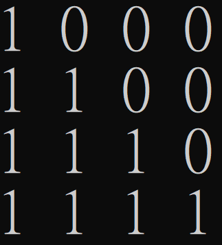
\(M_{DISJ}\)
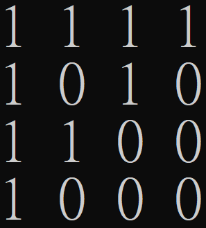
\(M_{IP}\)
Lower Bounds from Rank
\(M_{DISJ_2}\)
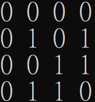
\(P= J-2M_{IP}\)
Lower Bounds from Rank
$$M_{DISJ_n} = \begin{bmatrix} 1&1 \\ 1&0\end{bmatrix} \otimes M_{DISJ_{n-1}}$$
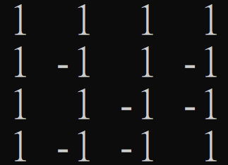
$$P_{n} = \begin{bmatrix} 1&1 \\ 1&-1\end{bmatrix} \otimes P_{n-1}$$
$${\rm rank}(M_{IP_n}) \geq {\rm rank} (P_n) - {\rm rank} (J_n)$$
Randomized
Public VS Private Coin
private-coin protocol of length \(c\) \(\implies\) public-coin protocol of length \(c\)
public-coin protocol of length \(c\) \(\implies\) private-coin protocol of length \(O(c+\log n)\)
(Newman's Theorem)
Randomized Protocol
=
Distribution of Deterministic Protocols
Distributional Complexity
von Neumann's minimax principle: For a \(n\times m\) matrix \(M\),
$$\max\limits_{x\in \mathbb R^n, ||x||_1 =1, x_i > 0} \min\limits_{y\in \mathbb R^m, ||y||_1 =1, y_i > 0} x^T M y = \min_y \max_x x^T M y$$
The randomized complexity of \(f,\epsilon\) is at least \(c\)
\(\Leftrightarrow\)
There is a distribution \(D\) of inputs \((x,y)\) such that for all deterministic protocol \(\pi\) with error \(\epsilon\), the length of \(\pi\) on \(D\) is at least \(c\)
\(\infty \star\) Yao's(姚期智) Principle

Discrepancy
For a set \(S\subseteq \mathcal X \times \mathcal Y\), and a distribution \(\mu\) over the inputs, we say the discrepancy of \(f(x,y)\) w.r.t. \(S\) and \(\mu\) is
$$|\mathbb E_\mu [\chi_S(x,y)(-1)^{f(x,y)}]|$$
low discrepancy for every rectangle \(\implies\) high communication complexity?
For a distribution \(\mu\), if the discrepancy of \(f\) w.r.t. every rectangle is at most \(\gamma\), then the length of any ptotocol computing \(f\) with error \(\epsilon\) is at least \(\log(\frac{1-2\epsilon}{\gamma})\) when inputs are drawn from \(\mu\).
Randomized Lower Bound of IP
For every rectangle \(R \subseteq \mathcal X \times \mathcal Y\),
$$|\mathbb E_U[\chi_{R}(x,y) (-1)^{IP(x,y)}]| \leq \sqrt{2^{-n}}$$
The randomized communication complexity of IP is at least \(\frac{n}{2}-\log(\frac{1}{1-2\epsilon})\) (\(\Omega(n)\))
Randomized Lower Bound of DISJ
\(\Omega(n)\)
\(\Omega(n)\)
\(\Omega(n)\)
\(\infty \star !!!\)
Why study communication complexity?
Applications
VLSI Time-Space Tradeoff
Proof Complexity
Formula Lower Bounds
Pseudo-randomness...
Space Complexity of Streaming Models
Data Structures
Extension Complexity
Extension Complexity
E.R. Swart. P=NP. Report No. CIS86-02, Department of Computer and Information Science, University of Guelph, Ontario, Canada, 1986
(參考圖片,非當事論文)
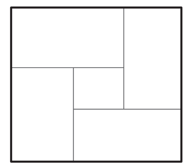
Polytope
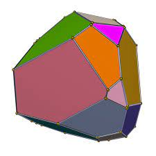
Intersection of several half-spaces(linear inequalities), and can be expressed as \(P:=\{x|Ax \leq b\}\).
face(generated by some supporting hyperplane)
vertex(also a face)
facet(also a face)
Example
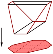
By adding auxiliary variables, we obtain an extension of the original polytope.
extension
projection
Example
The extension complexity of a polytope \(P\) is the minimum number of facets(inequalities) achieved by any extension of \(P\).
extension
projection
What is \(xc(TSP(n))\)?
Nondeterministic Communication Complexity
The setting is the same, A gets \(x\) and B gets \(y\). However, a person C knows both \(x\) and \(y\), and C needs to convince A and B that \(f(x,y)=1\).
The nondeterministic communication complexity of NEQ is \(O(\log n)\).
The nondeterministic communication complexity of EQ is \(\Omega(n)\).
1-rectangle cover
If there is a 1-rectangle cover of size \(t\) of \(M_f\), then there is a nondeterministic protocol of size \(\log t\).
If there is a nondeterministic protocol of length \(c\) for \(f\), then \(M_f\) can be covered by \(2^c\) rectangles.
What is the nondeterministic communication complexity of DISJ?
Extension and Nondeterministic Communication?
\(xc(P) = r\)
\(rank_+(S) = r\), where \(S\) is the slack matrix of \(P\).
The nondeterministic communication complexity of Face-Vertex(P) is \(O(\log r)\).
\(\implies\)
Yannakakis' Factorization Theorem
\(\Leftrightarrow\)
Slack Matrix
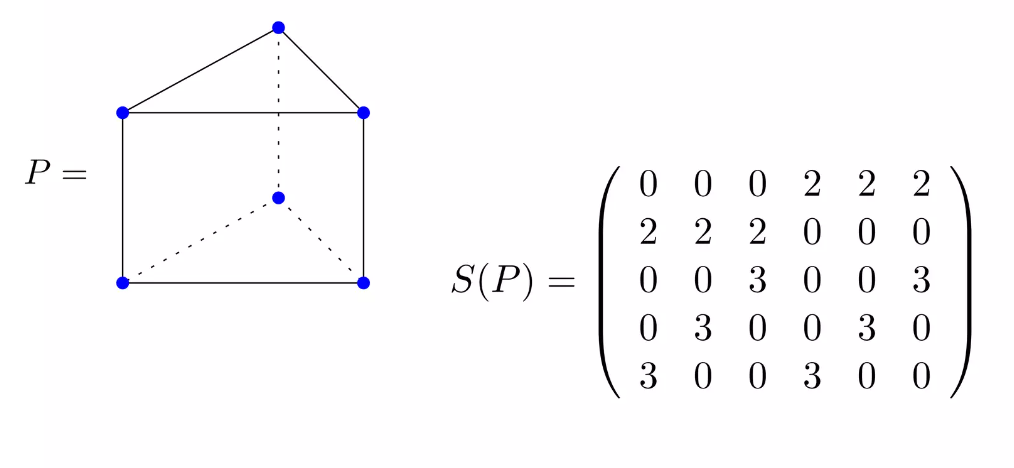
A slack matrix \(S\) of \(P\) is a \(|F| \times |V|\) matrix, where \(F\) is the set of faces, and \(V\) is the set of vertices.
\(S_{fv} = q_f-p_f^Tx_v\), where \(p_f^Tx \leq q_f\) is the supporting hyperplane of the \(f\)-th face.
Yannakakis' Factorization Theorem-1
\(xc(P) \leq rank_+(S)\)
Suppose \(rank_+(S)=r\), then we can write \(S = RT\), where \(R_{|F|\times r}, T_{r\times |V|}\) are nonegative.
We collect the supporting hyperplanes for every face of \(P\), and obtain \(A'x \leq b'\), which is in fact \(P\) itself, and \(S^i = b'-A'v_i\).
Let \(Q:=\{(x,y)|A'x+Ry = b',y \geq 0\}\), which has only \(r\) inequalities, and \(proj_x(Q)\subseteq P\).
Also \(P\subseteq proj_x(Q)\), because for every vertex \(v_i\) of \(P\), \((v_i,T^i) \in Q\).
Yannakakis' Factorization Theorem-2
\(xc(P) \geq rank_+(S)\)
Suppose \(xc(P)=r\), and \(Q:=\{(x,y)|Cx + Dy \leq d\}\) is an extension of \(P:\{x|Ax \leq b\}\).
Farkas Lemma: Either \(Ax\leq b\) has a solution \(x\) with \(x \in \mathbb R^n\), or \(A^Ty = 0\) has a solution \(y\) with \(y \geq 0,y^Tb < 0\).
Each supporting hyperplane generating each face of Q can be expressed as some nonegative linear combination of the facets of \(Q\).
\(\implies\)
Yannakakis' Factorization Theorem-2
\(xc(P) \geq rank_+(S)\)
Suppose \(xc(P)=r\), and \(Q:=\{(x,y)|Cx + Dy \leq d\}\) is an extension of \(P:\{x|Ax \leq b\}\).
Each supporting hyperplane generating each face of P can be expressed as some nonegative linear combination of the facets of \(Q\).
For the \(f\)-th face of \(P\) (generated by \(p_f^T x \leq q_f\)), we can find \(\lambda_f \in \mathbb R^r_+\), such that \(\lambda_f^T C = p^T, \lambda_f^T D = 0,\lambda_f^T d = q\).
For the \(v\)-th vertex (\(x_v\)) of \(P\), we can find \((x_v,y_v) \in Q\), and let \(\mu_v = d-Cx_v-Dy_v \in \mathbb R^r_+\).
\(\lambda_f^T \mu_v =\lambda_f^T (d - Cx_v - Dy_v)=q_f - p^T_fx_v = S_{fv}\)
Extension and Nondeterministic Communication
\(xc(P) = r\)
\(rank_+(S) = r\), where \(S\) is the slack matrix of \(P\).
The nondeterministic communication complexity of FACE-VERTEX(P) is \(O(\log r)\).
\(\implies\)
Yannakakis' Factorization Theorem
\(\Leftrightarrow\)
Example: Correlation Polytope
Define \(CORR(n)\) as the convex hull of \(\{y=x^Tx|x \in \{0,1\}^n\}\)
Can we prove the extension complexity of \(CORR(n)\)?
We should consider the nondeterministic communication complexity of \(FACE-VERTEX(CORR(n))\).
The Lemma
For every \(s \in \{0,1\}^n\), there exist a face \(f_s\) of \(CORR(n)\), such that \(\forall x \in \{0,1\}^n\)
$$y=x^Tx \in f_s \iff |s \cap x|=1$$
\(((\sum_{s_i = 1} x_i) -1)^2 \geq 0\) would be great, but it is not linear.
We change \(x_i\), \(x_i^2\) into \(y_{ii}\), and change \(2x_ix_j\) into \(y_{ij}+y_{ji}\) to obtain \(f_s\).
Reduction?
FACE-VERTEX(CORR(n))
SIZE-OF-INTERSECTION-IS-NOT-ONE(n)
UNIQUE-DISJ(n)
easier
easier
Only consider the faces mentioned in the lemma.
Only consider \((x,y)\) such that \(|x\cap y | \leq 1\)
Nondeterministic communication complexity of UNIQUE-DISJ!
UNIQUE-DISJ
UNIQUE-DISJ(2)
Still, we want to obtain a lower bound for the size of the 1-rectangle cover of \(M_{UNIQUE-DISJ}\).
1-rectangle size
Lemma: Each 1-rectangle in \(M_{UNIQUE-DISJ}\) contains at most \(2^n\) 1-inputs.
Induction hypothesis: For a 1-rectangle \(R = A\times B\), where all \(x\in A,y\in B\) have 0s in their last \(n-k\) coordinates, \(R\) contains at most \(2^k\) 1-inputs.
\(k = 0\) is obvious, and \(k=n\) is what we want.
1-rectangle size
Induction hypothesis: For a 1-rectangle \(R = A\times B\), where all \(x\in A,y\in B\) have 0s in their last \(n-k\) coordinates, \(R\) contains at most \(2^k\) 1-inputs.
For \(k>0\), given \(R\), we want to construct two sets of 1-inputs \(S_1,S_2\), such that
1. \(rect(S_1),rect(S_2)\) are 1-rectangles and have 0s in their last \(n-k+1\) coordinates.
2. the number of 1-entries in \(S_1,S_2\) is at least the number of 1-inputs in \(R\).
We can get rid of of the last \(n-k\) coordinates.
1-rectangle size
1. \(rect(S_1),rect(S_2)\) are 1-rectangles and have 0s in their last \(n-k+1\) coordinates.
2. The number of 1-entries in \(S_1,S_2\) is at least the number of 1-inputs in \(R\).
Note that \((a1,b1)\) is not an 1-input, and \((a0,b1),(a1,b0)\) will not be in \(R\) at the same time if \((a0,b0)\) is an 1-input.
For every 1-input in \(R\),
\((a0,b1) \implies\) put it in \(S_1'\)
\((a1,b0) \implies\) put it in \(S_2'\)
\((a0,b0) \implies\) put it in \(S_1'\) if \((a_0,b_1)\notin R\), put it in \(S_2'\) if \((a_1,b_0)\notin R\)
\(rect(S_i')\)s are 1-rectangles.
\(x_k = 0\) in \(rect(S_1')\), \(y_k = 0\) in \(rect(S_2')\)
1-rectangle size
Obtain \(S_i\) by setting \(y_k = 0\) in \(rect(S_1')\) and \(x_k = 0\) in \(rect(S_2')\)
\(rect(S_i')\)s are 1-rectangles.
\(x_k = 0\) in \(rect(S_1')\), \(y_k = 0\) in \(rect(S_2')\)
\(|S_i| = |S_i'|\)
1. \(rect(S_1),rect(S_2)\) are 1-rectangles and have 0s in their last \(n-k+1\) coordinates.
2. The number of 1-entries in \(S_1,S_2\) is at least the number of 1-inputs in \(R\).
\(rect(S_i)\) have 0s in their last \(n-k+1\) coordinates.
\(rect(S_i)\)s are 1-rectangles.
Proof Complete!
1-rectangle cover
Lemma: Each 1-rectangle in \(M_{UNIQUE-DISJ(n)}\) contains at most \(2^n\) 1-inputs.
Besides, we know that there are \(3^n\) 1-inputs in \(M_{UNIQUE-DISJ(n)}\).
Thus, any 1-rectangle cover has size at least \((1.5)^n\), and the nondeterministic communication complexity of UNIQUE-DISJ(n) would be \(\Omega(n)\).
So, finally,
$$xc(CORR(n)) = 2^{\Omega(n)}$$
How about \(TSP(n)\)?
\(TSP(n) = {\rm conv}\{\chi_F \in \{0,1\}^{|E(K_n)|}|F \subseteq E(K_n) \text{is a tour of } K_n \}\)
There is a face of \(TSP(cn^2)\) that is an extension of \(CORR(n)\).
\(\{x^Tx|x \in \{0,1\}^n\}\)
The satisfying assingments of \(\phi_n := \land_{i,j\in[n],i\neq j} (C_{ij} = C_{ii} \land C_{jj})\)
(\(O(n^2)\) variables and clauses)
Halmiltonian cycle of some directed graph \(D_n\)
(\(O(n^2)\) vertices and edges)
Halmiltonian cycle of some undirected graph \(G_n\)
(\(O(n^2)\) vertices and edges)
\(\iff\)
\(\iff\)
\(\iff\)
There is a face of \(TSP(cn^2)\) that is an extension of \(CORR(n)\).
Extension Complexity of TSP(n)
If \(Q\) is an extension of \(P\), then \(xc(Q)\geq xc(P)\)
If \(P\) is a face of \(Q\), then \(xc(Q)\geq xc(P)\)
(Consider the slack matrix.)
There is a face of \(TSP(cn^2)\) that is an extension of \(CORR(n)\).
The extension complexity of \(TSP(n)\) is \(2^{\Omega(\sqrt n)}\) ><
Q
References
[1] T. Roughgarden. Communication complexity (for algorithm designers). Foundations and Trends in Theoretical Computer Science, 11(3–4):217–404, 2016.
[2] Mathematics and Computation: A Theory Revolutionizing Technology and Science (Princeton University Press, October 2019)
[3] Rao, A., & Yehudayoff, A. (2020). Communication Complexity: And Applications. Cambridge: Cambridge University Press. doi:10.1017/9781108671644
[4] Samuel Fiorini, Serge Massar, Sebastian Pokutta, Hans Raj Tiwary, and Ronald de Wolf. 2015. Exponential Lower Bounds for Polytopes in Combinatorial Optimization. J. ACM 62, 2, Article 17 (May 2015), 23 pages. https://doi.org/10.1145/2716307
Kolmogorov Complexity and the Incompressibility Method
What's the next number?
\(1,2,4,8,16,\)
What's the next number?
\(1,2,4,8,16,\)
\(7122\)?
\(32\)?
What is randomness?
\(1,2,4,8,16,7122\)
\(1,2,4,8,16,32\)
k = 1
for i in range(5):
  print(k)
  k *= 2
k = 1
for i in range(4):
print(k)
k *= 2
print(7122)A = [1,2,4,8,16,7122]
for i in range(5):
print(A[i])Kolmogorov Complexity
\(C(x) = \min\{l(p):p \text{ is an encoding/program of }x\}\)
Think of \(x,p\) as binary strings(or natural numbers).
Kolmogorov Complexity
\(C(x) = \min\{l(p):p \text{ is an encoding/program of }x\}\)
Think of \(x,p\) as binary strings(or natural numbers).
A more formal definition
\(C_f(x) = \min\{l(p):f(p) = x\}\)
Where \(f\) is some (partial) function.
Kolmogorov Complexity
\(C(x) = \min\{l(p):p \text{ is an encoding/program of }x\}\)
Think of \(x,p\) as binary strings(or natural numbers).
A more formal definition
\(C_f(x) = \min\{l(p):f(p) = x\}\)
Where \(f\) is some (partial) function.
How should we choose \(f\)? (C++, python, Eric Xiao, ...?)
Kolmogorov Complexity
Maybe \(f\) should be the "minimal" (additively optimal) function:
\(\forall g,x, C_f(x) \leq C_g(x) + c_g\)
Kolmogorov Complexity
Such \(f\) doesn't exist:
Let \(g(i) = x_i\), where \(C_f(x_i) \geq i\)
Maybe \(f\) should be the "minimal" (additively optimal) function:
\(\forall g,x, C_f(x) \leq C_g(x) + c_g\)
Kolmogorov Complexity
Perhaps we should not consider all functions.
Kolmogorov Complexity
Perhaps we should not consider all functions.
Computable functions?
Kolmogorov Complexity
Perhaps we should not consider all functions.
Computable functions?
Let \(f_0\) be a function computed by a universal TM (\(T_0\)) with input \(11..110np\) (with \(l(n)\) ones ) which simulates \(T_n\) on input \(p\)
Kolmogorov Complexity
Perhaps we should not consider all functions.
Computable functions?
Let \(f_0\) be a function computed by a universal TM (\(T_0\)) with input \(11..110np\) (with \(l(n)\) ones ) which simulates \(T_n\) on input \(p\)
We have \(C_{f_0}(x) \leq C_{f_n}(x) + 2l(n)+1\)
\(f_0\) is additively optimal!
Kolmogorov Complexity
\(C(x) = C_{f_0}(x) = \min\{l(p):f_0(p) = x\}\)
Kolmogorov Complexity
\(C(x) = C_{f_0}(x) = \min\{l(p):f_0(p) = x\}\)
We can view \(f_0\) as a special compiler.
Is the compiler of C/Java additively optimal?
Conditional Kolmogorov Complexity
\(C(x|y) = C_{f_0}(x|y) = \min\{l(p):f_0(\langle y,p\rangle) = x\}\)
\(C(x) = C(x|\epsilon)\)
We also have \(\forall f,x,y\)
\(C_{f_0}(x|y) \leq C_f(x|y) + c_f \)
Upper bounds
\(\forall x,C(x) \leq l(x) + c\)
\(\forall x,y,C(x|y) \leq C(x)+c\)
Uncomputability
\(C(x)\) is uncomputable
function GenerateComplexString()
    for i = 1 to infinity:
        for each string s of length exactly i
            if KolmogorovComplexity(s) ≥ 8000000000
                return s
(Assume the length of KolmogorovComplexity() is \(700000000\))
Uncomputability
\(C(x)\) is uncomputable
function GenerateComplexString()
    for i = 1 to infinity:
        for each string s of length exactly i
            if KolmogorovComplexity(s) ≥ 8000000000
                return s
(Assume the length of KolmogorovComplexity() is \(700000000\))
「不能用二十個字以內描述的最小數字」
Uncomputability
\(C(x)\) is uncomputable on any infinite set of points
function GenerateComplexString()
    for i = 1 to infinity:
        for each string s of length exactly i
            if KolmogorovComplexity(s) ≥ 8000000000
                return s
(Assume the length of KolmogorovComplexity() is \(700000000\))
「不能用二十個字以內描述的最小數字」
Incompressibility Theorem \(\infty \star\)
Let \(c \in \mathbb N\) and \(A\) be a set of size \(m\),
then there are at least \(m(1-2^{-c})+1\) elements \(x\in A\) such that
\(C(x|y) \geq \log m -c\), for any fixed \(y\).
Incompressibility Theorem \(\infty \star\)
Let \(c \in \mathbb N\) and \(A\) be a set of size \(m\),
then there are at least \(m(1-2^{-c})+1\) elements \(x\in A\) such that
\(C(x|y) \geq \log m -c\), for any fixed \(y\).
Because there are only \(\sum\limits_{i=0}^{\log m-c-1} 2^i= m2^{-c}-1\) programs with length less than \(\log m-c\).
Example - Infinite Primes
Assume that there are only \(k\) primes. Then for each \(n \in \mathbb N\), we can write \(n = \prod\limits_{i=1}^k p_i^{\alpha_i}\). Thus we can describe every number in \([1,t]\) by \(k \log\log t\) bits......
Incompressity theorem: Let \(c \in \mathbb N\) and \(A\) be a set of size \(m\),
then there are at least \(m(1-2^{-c})+1\) elements \(x\in A\) such that
\(C(x|y) \geq \log m -c\), for any fixed \(y\).
\(\pi(n) \in \Omega(\frac{\log n}{\log \log n})\)
Example - TM complexity
Checking if a string is palindrome needs \(\Omega(n^2)\) time for any one-tape Turing Machine.
Example - TM complexity
Checking if a string is palindrome needs \(\Omega(n^2)\) time for any one-tape Turing Machine.
Assume a TM \(T\):
- each state can be described by \(\ell\) bits
- always terminates with the reading head at the rightmost position of the input
- computes PALINDROME
Example - TM complexity
Checking if a string is palindrome needs \(\Omega(n^2)\) time for any one-tape Turing Machine.
Assume a TM \(T\):
- each state can be described by \(\ell\) bits
- always terminates with the reading head at the rightmost position of the input
- computes PALINDROME
Define the crossing seuence of a grid \(g\): the sequence of states of the TM \(T\) when the reading head crosses the right boundary of \(g\)
Example - TM complexity
By the incompressibility theorem, we can find length-\(n\) string \(x\) with \(C(x|T,n) \geq n\).
Example - TM complexity
By the incompressibility theorem, we can find length-\(n\) string \(x\) with \(C(x|T,n) \geq n\).
Consider running \(T\) on \(x 0^{2n} \bar x\), if the runtime is less than \(\frac{n^2}{\ell}\), then there exists a "middle" grid \(g_0\) with crossing sequence shorter than \(\frac{n}{2 \ell}\).
In fact, given \(T,n\), we can recover \(x\) by the position of \(g_0\)(\(\frac{n}{2}\) bits) and the crossing sequence of \(g_0\)(\(O(\log n)\) bits).
\(C(x|T,n) \leq \frac{n}{2} + O(\log n)\)
Example - TM complexity
We can recover \(x\) by checking if the crossing sequence at \(g_0\) with input \(y0^{2n} \bar x\) is the same as \(x0^{2n} \bar x\) for all \(y \in \{0,1\}^n\) !
Example - TM complexity
We can recover \(x\) by checking if the crossing sequence at \(g_0\) with input \(y0^{2n} \bar x\) is the same as \(x0^{2n} \bar x\) for all \(y \in \{0,1\}^n\) !
How about average complexity?
Incompressibility Method
If the statement doesn't hold, then there will be too many compressible objects.
Combinatorial Properties
Some Useful Bounds
\(\dfrac {n^n} {e^{n - 1} } \le n! \le \dfrac {n^{n + 1} } {e^{n - 1} }\)
\(\left({\frac{n}{k}}\right)^{k}\leq C^n_k\leq{\frac{n^{k}}{k!}}\lt \left({\frac{n e}{k}}\right)^{k}\)
Transitive Tournament
Tournament: complete directed graph
Transitive tournament: acyclic tournament
\(v(n):\) Largest integer such that every tournament on \(n\) nodes contains a subtournament on \(v(n)\) nodes.
Transitive Tournament
Tournament: complete directed graph
Transitive tournament: acyclic tournament
\(v(n):\) Largest integer such that every tournament on \(n\) nodes contains a subtournament on \(v(n)\) nodes.
\(\lfloor \log n \rfloor \leq \)\(v(n) \leq 1 + \lfloor 2\log n \rfloor\)
Counting
\(v(n) \leq 1 + \lfloor 2\log n \rfloor\)
\(v:= 2 + \lfloor 2\log n \rfloor\)
\(A:\) subset of \([n]\) of size \(v\)
\(\sigma:\) permutation on \([v]\)
\(\Gamma_{A,\sigma}:\) the set of \(n\)- vertex tournaments of whom \(A\) is a subtournament with "order" \(\sigma\)
We count the number \(d(\Gamma')\) of \(n\)- vertex tournaments with a transitive subtournament of size \(v\)
\(d(\Gamma') \leq \sum_A \sum_\sigma d(\Gamma_{A,\sigma}) = C^n_v v! 2^{C^n_2-C^v_2} < 2^{C^n_2}\)
\( (C^n_v v! < n^v \leq 2^{C^v_2})\)
Probabilistic Method
\(v(n) \leq 1 + \lfloor 2\log n \rfloor\)
\(v:= 2 + \lfloor 2\log n \rfloor\)
\(A:\) subset of \([n]\) of size \(v\)
\(\sigma:\) permutation on \([v]\)
Let \(T\) be the random variable uniformly distributed over all \(n\)-vertex tournaments.
We calculate the probability \(P(T\in \Gamma')\).
\(P(T\in \Gamma') \leq \sum_A \sum_\sigma P(T \in \Gamma_{A,\sigma}) = C^n_v v! 2^{-C^v_2} < 1\)
\( (C^n_v v! < n^v \leq 2^{C^v_2})\)
Incompressibility Method
\(v(n) \leq 1 + \lfloor 2\log n \rfloor\)
If \(v(n)\) is too large, then we can compress every \(n\)-vertex tournament. (contradicting the incompressibility theorem)
Formally speaking, by the incompressibility method, there is some tournament \(T'\), where \(C(T'|n,p) \geq n(n-1)/2\).
(\(p\) is some decoding program)
However, for every tournament \(T\), we can describe it by \(v(n) \lfloor \log n \rfloor+ n(n-1)/2 - v(n)(v(n)-1)/2\) bits.
Thus \(v(n) \lfloor \log n \rfloor - v(n)(v(n)-1)/2 \geq 0\), and
\(v(n) \leq 2 \lfloor \log n\rfloor + 1\).
Incompressibility Method
In fact, by the incompressibility method, we can also prove:
For at least a (\(1 - \frac{1}{n}\))th fraction of \(n\)-vertex tournaments, the largest transitive subtournament has at most \((1 + 2\lfloor 2\log n\rfloor)\) nodes for \(n\) large enough.
\(v(n) \leq 1 + \lfloor 2\log n \rfloor\)
Excerises
1. Give an upper bound for \(w(n)\), the largest integer such that for each \(n\)-vertex tournament \(T\), there are two disjoint subsets of vertices \(A,B\), each of size \(w(n)\), and \(A \times B \in T\).
// x,y are n-bit
s = (x ^ y)
c = (x & y)
while c != 0:
  s' = (s ^ c)
  c' = (s & c)
  s = s'
  c = c'
2. Prove that the while loop loops at most \(\log n + 1\) steps in average:
4. What are the differences between the counting argument, the probabilistic method, and the incompressibility method?
5. Ask a question.
3. Prove that almost all \(n\)-vertex labeled trees have maximum degree \(O(\frac{\log n}{\log \log n})\).
W.W. Kirchherr, Kolmogorov complexity and random graphs
Time Complexity
Shell Sort
\(h_1,h_2,...,h_p=1\)
In the \(i-\)th pass, divide the list into \(h_i\) sublists (by (\(p \mod h_i\))) and do insertion sort.
\(h = [5,3,1]\):
Average Time Complexity of Shell Sort
Pratt: \(\Theta(n \log^2 n)\) (worst case also), using \(h_k \in \{2^i 3 ^j|2^i 3 ^j < \frac{N}{2}\}\)
Knuth: \(\Theta(n^{5/3})\), using the best choice of \(h\) for \(p=2\)
Yao, Janson, Knuth: \(O(n^{23/15})\), using some choice of \(h\) for \(p=3\)
We prove that running shell sort for any \(p\) and \((h_1,h_2,...,h_p)\), the time complexity is \(\Omega(pn^{1+1/p})\).
Proof Outline
Fix some permutation \(\pi\) such that \(C(\pi|n, A,p) \leq \log n! - \log n\),
where \(A\) is the algorithm, and \(p\) is some decoding program.
*A fraction of \((1 - \frac{1}{n})\) permutations satisfy this condition.
Let \(m_{i,k}\) be the distance that the number \(i\) moved in pass \(k\), and \(M = \sum\limits_{i=1}^n \sum\limits_{k=1}^p m_{i,k}\), which is a lower bound of the runtime.
By all \(m_{i,k}\), we can recover \(\pi\).
If \(M = o(pn^{1+1/p})\), we can express all \(m_{i,k}\) with too few bits. (TBD)
Thus the runtime is \(\Omega(pn^{1+1/p})\) for a fraction of \((1-\frac{1}{n})\) permutations and so is the average runtime.
Proof Detail
To describe all \(m_{i,k}\), we can descibe
the sum of them (\(M\), described by \(O(\log n)\) bits), and
the way of partitioning \(M\) into \(np\) parts (described by \(\log (H^{np}_M)\) bits).
Thus \(\log (H^{np}_M) + O(\log n) \geq \log n! - \log n\),
$$\log(C^{M+np-1}_{np-1}) \geq \log n! + O(\log n)$$
\((np-1)[\log(\frac{M}{np-1}+1)+\log e] \geq n\log n - n \log \mathrm e + O(\log n)\)
(using \(C^n_k \leq \left({\frac{n e}{k}}\right)^{k} \) and \(n! \geq \frac{n^n}{e^n}\))
Thus \(M = \Omega(pn^{1+1/p})\) ???
Regular Language
Regular Language
A language accepted by some DFA.

Pumping Lemma
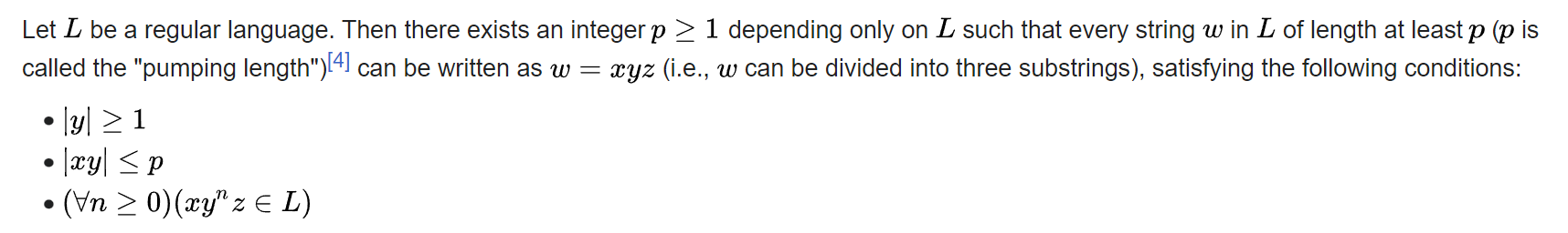
Pumping Lemma
Might not be easy to use.
Not characterizing.
Example
Is \(L := \{0^k 1^k | k \geq 1\}\) a regular language?
Example
Is \(L := \{0^k 1^k | k \geq 1\}\) a regular language?
Suppose \(L\) is accepted by some DFA \(A\). Then we can recover \(k\) from \(A\) and \(q\), the state of \(A\) after processing \(0^k\). Thus for all \(k\geq 1\), \(C(k) \leq O(1)\).
KC-Regularity
Suppose \(L\) is regular, and \(L_x := \{y|xy \in L \}\). If \(y\) is the \(n\)-th string in \(L_x\), then \(C(y) \leq C(n) + O(1)\).
KC-Regularity
Suppose \(L\) is regular, and \(L_x := \{y|xy \in L \}\). If \(y\) is the \(n\)-th string in \(L_x\), then \(C(y) \leq C(n) + O(1)\).
*What does "the \(n\)-th string" mean?
More Examples
Is \(L := \{1^p |p\text{ is prime}\}\) a regular language?
Is \(L := \{x \bar x w \large ||x|,|w| > 0\}\) a regular language?
Regular KC-Characterization
In fact, we have
\(L\) is regular
\(\Leftrightarrow\)
Exists \(c_L\), such that for all \(x,n\), \(C(\chi^x_{1:n}) \leq C(n) + c_L\)
For all \(x,n\), if \(y\) is the \(n\)-th string in \(L_x\), then \(C(y) \leq C(n) + O(1)\).
\(\Leftrightarrow\)
Regular KC-Characterization
In fact, we have
\(L\) is regular
\(\Leftrightarrow\)
Exists \(c_L\), such that for all \(x,n\), \(C(\chi^x_{1:n}) \leq C(n) + c_L\)
For all \(x,n\), if \(y\) is the \(n\)-th string in \(L_x\), then \(C(y) \leq C(n) + O(1)\).
\(\Leftrightarrow\)
Thus, (in theory), we can prove non-regularity of every non-regular language and regularity of every regular language.
Last Example
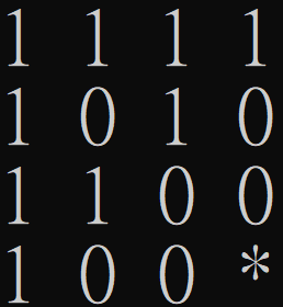
Is \(L := \{x |\sum x_i = 2k+1\}\) a regular language?
Last Example
Is \(L := \{x |\sum x_i = 2k+1\}\) a regular language?
There exists \(c_L\), such that for all \(x,n\), \(C(\chi^x_{1:n}) \leq C(n) + c_L\).
Excerises
1. Prove (or disprove) that \(L:=\{0^i 1^j|\gcd(i,j) = 1\}\) is regular.
2. Alice and Bob are playing the number guessing game. Alice chooses some \(x \in [n]\), and Bob can ask her yes/no questions. If Alice can lie once, what is the minimum number \(c\) where Bob can always guess the right answer after asking \(c\) questions?
5. Why is computability important?
6. Ask a question.
4. Prove any (nontrivial?) statement via the incompressibility method.
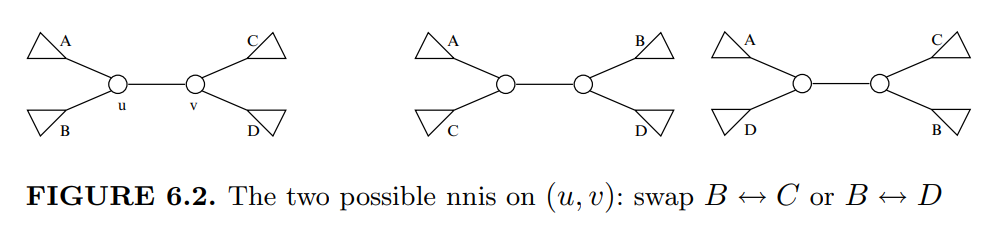
3. An nni (nearest-neighbor interchange) operation can be done on neighboring internal nodes on an evolutionary tree. Let \(f(A,B)\) denote the nni-distance between two \(n\)-node evolutionary trees. Prove that \(\max_{A,B} f(A,B) = \Omega(n \log n)\). (In fact, \(\Theta(n \log n)\).)
References
[1] Wikipedia contributors. (2023, March 5). Incompressibility method. In Wikipedia, The Free Encyclopedia. Retrieved 15:03, August 27, 2023, from https://en.wikipedia.org/w/index.php?title=Incompressibility_method&oldid=1143081380
[2] Wikipedia contributors. (2023, August 22). Kolmogorov complexity. In Wikipedia, The Free Encyclopedia. Retrieved 15:03, August 27, 2023, from https://en.wikipedia.org/w/index.php?title=Kolmogorov_complexity&oldid=1171617849
[3] Ming Li , Paul Vitányi. An Introduction to Kolmogorov Complexity and Its Applications, 2008.
A Glimpse into
Algorithmic Game Theory
2024.2.15
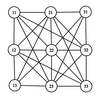
Other Considerd Topics - Spectral Graph Theory
- Spectrum of Adjacency Matrix/Laplacian
- Expander Graphs/PSRGs
- Expander Codes
- Nearly-linear time Laplacian solvers
Other Considerd Topics - Sum of Squares Hierachy
- Semidefinite Programming/Polynomial Optimization?
- polynomial-time 0.878-approximation algorithm for max cut (and why this might be optimal)
Today's Topic - Algorithmic Game Theory
- Auction Analysis
- Price of Anarchy (PoA, 最壞均衡與最佳解比)
Reference (mostly by Tim Roughgarden):
Barbados Lectures on Complexity Theory, Game Theory, and Economics
What is a Game?
A game is defined by
1. A set of \(n\) players
2. The pure strategy set for each player: \(S_1,S_2,...,S_n\)
3. The payoff function for each player: \(u_1, u_2, ..., u_n : S_1 \times S_2 \times ... \times S_n \to \mathbb R\)
https://www.youtube.com/watch?app=desktop&v=-1GDMXoMdaY
Equilibriums
A pure strategy profile \(s^* \in S_1\times S_2\times ... \times S_n\) is a Pure Nash Equilibrium (PNE) if
\({ u}_{i}\left(s^*\right)\,\ge\,{u}_{i}\left(s_{i}\,,\,s_{-i}^{\ast}\right)\, \forall i\in [n] \text{ and }s_i \in S_i\)
A mixed strategy profile \(p^* \in \Delta(S_1)\times \Delta(S_2)\times ... \times \Delta(S_n)\) is a Mixed Nash Equilibrium (MNE) if
\(\mathbb E_{s^* \sim p^*}[{ u}_{i}\left(s^*\right)]\,\ge\,\mathbb E_{s_{-i}^*\sim p^*_{-i}}[{u}_{i}\left(s_{i}\,,\,s_{-i}^{\ast}\right)]\, \forall i\in [n] \text{ and }s_i \in S_i\)
Nash's theorem: There is at least one MNE for each game.
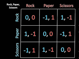
Q: What is an MNE for two-player rock paper scissors?
Equilibriums
A pure strategy profile \(s^* \in S_1\times S_2\times ... \times S_n\) is a Pure Nash Equilibrium (PNE) if
\({ u}_{i}\left(s^*\right)\,\ge\,{u}_{i}\left(s_{i}\,,\,s_{-i}^{\ast}\right)\, \forall i\in [n] \text{ and }s_i \in S_i\)
A mixed strategy profile \(p^* \in \Delta(S_1)\times \Delta(S_2)\times ... \times \Delta(S_n)\) is a Mixed Nash Equilibrium (MNE) if
\(\mathbb E_{s^* \sim p^*}[{ u}_{i}\left(s^*\right)]\,\ge\,\mathbb E_{s_{-i}^*\sim p^*_{-i}}[{u}_{i}\left(s_{i}\,,\,s_{-i}^{\ast}\right)]\, \forall i\in [n] \text{ and }s_i \in S_i\)
Nash's theorem: There is at least one MNE for each game.
Q: Why are equilibriums important?
What is Economics?
What is Economics?
- 經世濟民
- 尋找最有效率分配資源的方式
An Efficient Auction Mechanism:
Single-Item Second-Price Auction
1. Each of the \(n\) bidders has a private valuation \(v_i\) of the item.
2. Each bidder submits its bid \(b_i\) to the auctioneer simultaneously.
3. The auctioneer gives the item to the \(k\)-th bidder where \(b_k=\max_{i} b_i\) and charges \(p(b) = \max_{j\neq k} b_j\)
- Bidding truthfully \((b_i = v_i)\) maximizes the utility \(u_i(b) = (v_i -p(b)) \cdot [ i = k]\) for every bidder.
- The social welfare \(\mathrm{SW}(b) = v_{k}\) is always maximized when all bidders bid truthfully.
How about Single-Item First-Price Auctions?
1. Each of the \(n\) bidders has a private valuation \(v_i\) of the item.
2. Each bidder submits its bid \(b_i\) to the auctioneer simultaneously.
3. The auctioneer gives the item to the \(k\)-th bidder where \(b_k=\max_{i} b_i\) and charges \(b_k\)
How about Single-Item First-Price Auctions?
1. Each of the \(n\) bidders has a private valuation \(v_i\) of the item.
2. Each bidder submits its bid \(b_i\) to the auctioneer simultaneously.
3. The auctioneer gives the item to the \(k\)-th bidder where \(b_k=\max_{i} b_i\) and charges \(b_k\)
Q:What will the bidders' strategy be? Is the welfare always maximzied?
How about Single-Item First-Price Auctions?
1. Each of the \(n\) bidders has a private valuation \(v_i\) of the item.
2. Each bidder submits its bid \(b_i\) to the auctioneer simultaneously.
3. The auctioneer gives the item to the \(k\)-th bidder where \(b_k=\max_{i} b_i\) and charges \(b_k\)
Questions we will consider:
- How can we define the efficiency(inefficiency) of the first-price auction?
- How can we find/prove the efficiency of the first-price auction?
- Other kinds of auctions? More than one item?
Model:
Games(Auctions) of Incomplete Information
Assumption:
The valuation \(v_i\) of each bidder is drawn independently from some publicly-known distribution \(\cal F_i\). (\(\cal F_i\) Corresponds to the common beliefs that bidders have about everyone’s valuations.)
A strategy of the \(i\)-th bidder is a function \(s_i: \mathrm{SUPP}(\cal F_i) \to \mathbb R^+\). (When my valuation is \(v_i\) , I will bid \(s_i(v_i)\).)
A strategy profile \(s\) is a Bayes-Nash Equilibrium(BNE) if \(\forall i \in [n], v_i \in \mathrm{SUPP}(\cal F_i)\)
\(\mathbb E_{v_{-i} \sim \cal F_{-i}}[u_i(s(v_{-i},v_i))] \geq \mathbb E_{v_{-i} \sim \cal F_{-i}}[u_i(s_{-i}(v_{-i}),r')]\), \(\forall r' \in \mathbb R^+\)
Q : The mixed version?
Example:
Two bidders, symmetric uniform valuation
Q:
There are two bidders in a first-price auction, and \(v_1, v_2\) i.i.d. follow \(U[0,1]\). Please find a (pure) BNE.
Example:
Two bidders, symmetric uniform valuation
Q:
There are two bidders in a first-price auction, and \(v_1, v_2\) i.i.d. follow \(U[0,1]\). Please find a (pure) BNE.
Hint: The two bidders' strategies are identical and monotone.
Example:
Two bidders, symmetric uniform valuation
Q:
There are two bidders in a first-price auction, and \(v_1, v_2\) i.i.d. follow \(U[0,1]\). Please find a (pure) BNE.
Q:
Is the BNE easy to solve?
Does the BNE maximize the welfare?
Is the auction efficient in this case?
Example:
Two bidders, asymmetric uniform valuation
Q:
There are two bidders in a first-price auction, and \(v_1 \sim U[0,1], v_2\sim U[0,2]\) where \(v_1 \perp v_2\). Please find the BNE.
Example:
Two bidders, asymmetric uniform valuation
Q:
There are two bidders in a first-price auction, and \(v_1 \sim U[0,1], v_2\sim U[0,2]\) where \(v_1 \perp v_2\).
\(s_{1}(v_{1})=\;\frac{4}{3v_{1}}\left(1-\sqrt{1-\frac{3v_{1}^{2}}{4}}\right)\)
\(s_{2}(v_{2})=\;\frac{4}{3v_{2}}\left(\sqrt{1+\frac{3v_{2}^{2}}{4}}-1\right)\)
Example:
Two bidders, asymmetric uniform valuation
Q:
There are two bidders in a first-price auction, and \(v_1 \sim U[0,1], v_2\sim U[0,2]\) where \(v_1 \perp v_2\).
Q:
Is the BNE easy to solve?
Does the BNE maximize the welfare?
Is the auction efficient in this case?
\(s_{1}(v_{1})=\;\frac{4}{3v_{1}}\left(1-\sqrt{1-\frac{3v_{1}^{2}}{4}}\right)\)
\(s_{2}(v_{2})=\;\frac{4}{3v_{2}}\left(\sqrt{1+\frac{3v_{2}^{2}}{4}}-1\right)\)
Some notations
Valuation profile: \(v = (v_1, v_2, ..., v_n)\)
Bid profile: \(b = (b_1, b_2, ..., b_n)\)
Whether or not bidder \(i\) is the winner: \(x_i(b)\)
Selling price: \(p(b) = \max_i b_i\)
Utility: \(u_i(b,v_i)=(v_i-b_i) \cdot x_i(b)\)
Strategy profile: \(s = (s_1, s_2, ..., s_n): \mathrm{SUPP}(\cal F) \to \mathbb R^n\)
Social Welfare: \(\mathrm{SW}(b;v) = \sum\limits_{i=1}^n v_i \cdot x_i(b)\)
Whether or not bidder \(i\) has the highest valuation: \(x_i^*(v)\)
Optimal social welfare: \(\mathrm{OPT}(v) = \max_i v_i = \sum\limits_{i=1}^n v_i \cdot x_i^*(v)\)
\(\infty \star\) Price of Anarchy
Social Welfare: \(\mathrm{SW}(b;v) = \sum\limits_{i=1}^n v_i \cdot x_i(b)\)
Optimal social welfare: \(\mathrm{OPT}(v) = \max_i v_i\) \( = \sum\limits_{i=1}^n v_i \cdot x_i^*(v)\)
Price of Anarchy: \(\mathrm{PoA} = \min_{s \text{ is a BNE}} \frac{\mathbb E_{v \sim \cal F}[\mathrm{SW}(s(v);v)]}{\mathbb E_{v \sim \cal F}[\mathrm{OPT}(v)]} \)
High PoA \(\implies\) efficient auction?
Low PoA \(\implies\) inefficient auction?
Theorem 1
The PoA of first-price single-item auction is at least \(1-\frac{1}{e} \approx 0.63\).
Theorem 1
The PoA of first-price single-item auction is at least \(1-\frac{1}{e} \approx 0.63\).
Proof: We will proof the \(\frac{1}{2}\) PoA bound. There are two main inequalities.
Theorem 1
The PoA of first-price single-item auction is at least \(1-\frac{1}{e} \approx 0.63\).
Proof: We will proof the \(\frac{1}{2}\) PoA bound. There are two main inequalities.
1. For every valuation profile \(v\), bid profile \(b\), and bidder \(i\):
\(u_i(b_{-i},\frac{v_i}{2};v_i)\geq (\frac{1}{2} v_i - p(b))\)
Theorem 1
The PoA of first-price single-item auction is at least \(1-\frac{1}{e} \approx 0.63\).
Proof: We will proof the \(\frac{1}{2}\) PoA bound. There are two main inequalities.
1. For every valuation profile \(v\), bid profile \(b\), and bidder \(i\):
\(u_i(b_{-i},\frac{v_i}{2};v_i)\geq (\frac{1}{2} v_i - p(b))\cdot x_i^*(v)\)
2. For every BNE \(s\), bidder \(i\), and its valuation \(v_i\)
\(\mathbb{E}_{v_{-i}}\left[u_{i}({s}({v});v_{i})\right]\geq\mathbb{E}_{{v}_{-i}}\left[u_{i}(\frac{v_i}{2},{s}_{-i}({v}_{-i});v_{i})\right].\)
Theorem 1
The PoA of first-price single-item auction is at least \(1-\frac{1}{e} \approx 0.63\).
Proof: We will proof the \(\frac{1}{2}\) PoA bound. There are two main inequalities.
1. For every valuation profile \(v\), bid profile \(b\), and bidder \(i\):
\( \sum_i u_i(b_{-i},\frac{v_i}{2};v_i)\geq \sum_i(\frac{1}{2} v_i - p(b))\cdot x_i^*(v) = \frac{1}{2}\mathrm{OPT}(v)-p(b)\)
2. For every BNE \(s\), bidder \(i\),
\(\mathbb E_{v_i}\mathbb{E}_{v_{-i}}\left[u_{i}({s}({v});v_{i})\right]\geq\mathbb E_{v_i}\mathbb{E}_{{v}_{-i}}\left[u_{i}(\frac{v_i}{2},{s}_{-i}({v}_{-i});v_{i})\right].\)
Theorem 1
The PoA of first-price single-item auction is at least \(1-\frac{1}{e} \approx 0.63\).
Proof: We will proof the \(\frac{1}{2}\) PoA bound. There are two main inequalities.
1. For every valuation profile \(v\), bid profile \(b\), and bidder \(i\):
\( \sum_i u_i(b_{-i},\frac{v_i}{2};v_i)\geq \sum_i(\frac{1}{2} v_i - p(b))\cdot x_i^*(v) = \frac{1}{2}\mathrm{OPT}(v)-p(b)\)
2. For every BNE \(s\), bidder \(i\),
\(\mathbb{E}_{v}\left[u_{i}({s}({v});v_i)\right]\geq\mathbb{E}_{{v}}\left[u_{i}(\frac{v_i}{2},{s}_{-i}({v}_{-i});v_{i})\right].\)
Theorem 1
The PoA of first-price single-item auction is at least \(1-\frac{1}{e} \approx 0.63\).
Proof: We will proof the \(\frac{1}{2}\) PoA bound. There are two main inequalities.
1. For every valuation profile \(v\), bid profile \(b\), and bidder \(i\):
\( \sum_i u_i(b_{-i},\frac{v_i}{2};v_i)\geq \sum_i(\frac{1}{2} v_i - p(b))\cdot x_i^*(v) = \frac{1}{2}\mathrm{OPT}(v)-p(b)\)
2. For every BNE \(s\), bidder \(i\),
\(\mathbb{E}_{v} \sum_i\left[u_{i}({s}({v});v_i)\right]\geq\mathbb{E}_{{v}} \sum_i\left[u_{i}(\frac{v_i}{2},{s}_{-i}({v}_{-i});v_{i})\right].\)
Theorem 1
The PoA of first-price single-item auction is at least \(1-\frac{1}{e} \approx 0.63\).
Proof: We will proof the \(\frac{1}{2}\) PoA bound. There are two main inequalities.
1. For every valuation profile \(v\), bid profile \(b\), and bidder \(i\):
\( \sum_i u_i(b_{-i},\frac{v_i}{2};v_i)\geq \sum_i(\frac{1}{2} v_i - p(b))\cdot x_i^*(v) = \frac{1}{2}\mathrm{OPT}(v)-p(b)\)
2. For every BNE \(s\), bidder \(i\),
\(\mathbb E_v \mathrm{SW}(s(v);v) - p(s(v))=\mathbb{E}_{v} \sum_i\left[u_{i}({s}({v});v_i)\right]\geq\mathbb{E}_{{v}} \sum_i\left[u_{i}(\frac{v_i}{2},{s}_{-i}({v}_{-i});v_{i})\right].\)
\(\implies \mathrm{PoA} \geq \frac{1}{2}\)
Theorem 1
The PoA of first-price single-item auction is at least \(1-\frac{1}{e} \approx 0.63\).
* The \(1-\frac{1}{e}\) bound can be proved similarly.
* The bound holds even if the valuations are correlated!
More Items? Simultaneous First-price Auctions
1. Each of the \(n\) bidders has a private valuation \(v_{ij}(i \in [n], j \in [m])\) to each of the \(m\) item. (Assume \(v_i \sim \cal F_i\))
2. Each bidder submits its bid \(b_i = (b_{i1},b_{i2}, ..., b_{im})\) to the auctioneer simultaneously.
3. The auctioneer gives the \(j\)-th item to the \(k\)-th bidder where \(b_{kj}=\max_{i} b_{ij}\) and charges \(b_{kj}\)
Denote by \(S_i(b)\) the set of items given to bidder \(i\).
We assume the bidders are unit-demand:
\(u_i(b;v_i) = \max_{j \in S_i(b)} v_{ij} - \sum_{j \in S_i(b)} b_{ij}\)
Maximum weight matching?
Is there a PoA bound for
S1A with unit-demand bidders?
Theorem 2
The PoA of S1A with unit demand bidders is at least \(1-\frac{1}{e} \approx 0.63\).
Theorem 2
Every BNE of the S1A with unit-demand bidders and independent valuations achieves expected social welfare at least \(1 − \frac{1}{e}\) times the expected optimal welfare.
Theorem 2
Every BNE of the S1A with unit-demand bidders and independent valuations achieves expected social welfare at least \(1 − \frac{1}{e}\) times the expected optimal welfare.
We will first prove the complete-information version:
Every MNE of the S1A with unit-demand bidders and fixed valuations (\(\cal F_i\) is a degenarate distribution at \(v_i\)) achieves expected social welfare at least \(1 − \frac{1}{e}\) times the expected optimal welfare.
Theorem 2
Every MNE of the S1A with unit-demand bidders and fixed valuations (\(\cal F_i\) is a degenarate distribution at \(v_i\)) achieves expected social welfare at least \(1 − \frac{1}{e}\) times the expected optimal welfare.
Proof: (We will still prove the \(\frac{1}{2}\) PoA bound only.)
Denote by \(j^*(i)\), the item bidder \(i\) gets in some fixed optimal allocation. Define bidder \(i\)'s deviation \(b_i^*\) as bidding \(\frac{v_{ij^*(i)}}{2}\) on \(j^*(i)\) and \(0\) on other items.
Like the proof of theorem 1, we have for every bid profile \(b\),
\(u_{i}(b_{i}^{*},{b}_{-i}^{};\upsilon_{i})\,\ge\,\frac{v_{i j^{*}(i)}}{2}\,-\,p_{j^*(i)}(b)\)
Theorem 2
Every MNE of the S1A with unit-demand bidders and fixed valuations (\(\cal F_i\) is a degenarate distribution at \(v_i\)) achieves expected social welfare at least \(1 − \frac{1}{e}\) times the expected optimal welfare.
Proof: (We will still prove the \(\frac{1}{2}\) PoA bound only.)
Like the proof of theorem 1, we have for every bid profile \(b\),
\(u_{i}(b_{i}^{*},{b}_{-i}^{};\upsilon_{i})\,\ge\,\frac{v_{i j^{*}(i)}}{2}\,-\,p_{j^*(i)}(b)\)
Thus \(\sum_{i\in[n]}u_{i}(b_{i}^{*},{ b}_{-i};v_{i})\geq\frac{1}{2}\mathrm{OPT}({ v})-\sum_{j\in[m]}p_{j}({ b}).\)
Like the proof of theorem 1, using the definition of MNE, we can have PoA \(\geq \frac{1}{2}\).
Can we use the same proof for the incomplete-information case?
Theorem 2
Every BNE of the S1A with unit-demand bidders and independent valuations achieves expected social welfare at least \(1 − \frac{1}{e}\) times the expected optimal welfare.
Proof: (We will still prove the \(\frac{1}{2}\) PoA bound only.)
We fix some BNE, where bidder \(i\) samples its bid from the distribution \(D_i(v_i)\) when its valuation is \(v_i\). Denote by \(\cal G_i\) the distribution of bidder \(i\)'s bid, and \(\cal G = \cal G_1 \times \cal G_2 \times ... \times \cal G_n\).
We will use the randomized deviation \(b_i' \sim D_i'(v_i)\): sample \(v_{-i}\) from \(\cal F_{-i}\) and then performs \(b_i^*(v)\).
Theorem 2
Every BNE of the S1A with unit-demand bidders and independent valuations achieves expected social welfare at least \(1 − \frac{1}{e}\) times the expected optimal welfare.
Proof: (We will still prove the \(\frac{1}{2}\) PoA bound only.)
We will use the randomized deviation \(b_i' \sim D_i'(v_i)\): sample \(v_{-i}\) from \(\cal F_{-i}\) and then performs \(b_i^*(v)\).
By the definition of BNE, for every \(i\) and \(v_i\):
\(\mathbb E_{b_i \sim D(v_i), b_{-i} \sim \cal G_{-i}}[u_i(b;v_i)] \geq \) \(\mathbb E_{b_i' \sim D'(v_i), b_{-i} \sim \cal G_{-i}}[u_i(b_{-i},b_i';v_i)]\)
\(=\mathbb E_{v_{-i} \sim \cal F_{-i}, b_{-i} \sim \cal G_{-i}}[u_i(b_{-i},b_i^*(v);v_i)]\)
Theorem 2
Every BNE of the S1A with unit-demand bidders and independent valuations achieves expected social welfare at least \(1 − \frac{1}{e}\) times the expected optimal welfare.
Proof: (We will still prove the \(\frac{1}{2}\) PoA bound only.)
We will use the randomized deviation \(b_i' \sim D_i'(v_i)\): sample \(v_{-i}\) from \(\cal F_{-i}\) and then performs \(b_i^*(v)\).
By the definition of BNE, for every \(i\) and \(v_i\):
\(\mathbb E_{b_i \sim D(v_i), b_{-i} \sim \cal G_{-i}}[u_i(b;v_i)] \geq \) \(\mathbb E_{v_{-i} \sim \cal F_{-i}, b_{-i} \sim \cal G_{-i}}[u_i(b_{-i},b_i^*(v);v_i)]\)
Theorem 2
Every BNE of the S1A with unit-demand bidders and independent valuations achieves expected social welfare at least \(1 − \frac{1}{e}\) times the expected optimal welfare.
Proof: (We will still prove the \(\frac{1}{2}\) PoA bound only.)
We will use the randomized deviation \(b_i' \sim D_i'(v_i)\): sample \(v_{-i}\) from \(\cal F_{-i}\) and then performs \(b_i^*(v)\).
By the definition of BNE, for every \(i\):
\(\mathbb E_{v_i \sim \cal F_i,b_i \sim D(v_i), b_{-i} \sim \cal G_{-i}}[u_i(b;v_i)] \geq \) \(\mathbb E_{v \sim \cal F, b \sim \cal G}[u_i(b_{-i},b_i^*(v);v_i)]\)
Theorem 2
Every BNE of the S1A with unit-demand bidders and independent valuations achieves expected social welfare at least \(1 − \frac{1}{e}\) times the expected optimal welfare.
Proof: (We will still prove the \(\frac{1}{2}\) PoA bound only.)
We will use the randomized deviation \(b_i' \sim D_i'(v_i)\): sample \(v_{-i}\) from \(\cal F_{-i}\) and then performs \(b_i^*(v)\).
By the definition of BNE:
\(\sum_i \mathbb E_{v_i \sim \cal F_i,b_i \sim D(v_i), b_{-i} \sim \cal G_{-i}}[u_i(b;v_i)] \geq \) \(\mathbb E_{v \sim \cal F, b \sim \cal G}[\sum_i u_i(b_{-i},b_i^*(v);v_i)]\)
Last Proof:
\(\sum_{i}u_{i}(b_{i}^{*},{ b}_{-i};v_{i})\geq\frac{1}{2}\mathrm{OPT}({ v})-\sum_{j\in[m]}p_{j}({ b}).\)
Theorem 2
Every BNE of the S1A with unit-demand bidders and independent valuations achieves expected social welfare at least \(1 − \frac{1}{e}\) times the expected optimal welfare.
Proof: (We will still prove the \(\frac{1}{2}\) PoA bound only.)
We will use the randomized deviation \(b_i' \sim D_i'(v_i)\): sample \(v_{-i}\) from \(\cal F_{-i}\) and then performs \(b_i^*(v)\).
By the definition of BNE:
\(\mathbb E_{v \sim \cal F,b_i \sim D(v_i)\forall i}[\sum_i u_i(b;v_i)] \geq \) \(\frac{1}{2} \mathbb E_{v \sim \cal F}[\mathrm{OPT}(v)] - \mathbb E_{b \sim \cal G}[R(b)] \)
Theorem 2
Every BNE of the S1A with unit-demand bidders and independent valuations achieves expected social welfare at least \(1 − \frac{1}{e}\) times the expected optimal welfare.
Proof: (We will still prove the \(\frac{1}{2}\) PoA bound only.)
We will use the randomized deviation \(b_i' \sim D_i'(v_i)\): sample \(v_{-i}\) from \(\cal F_{-i}\) and then performs \(b_i^*(v)\).
By the definition of BNE:
\(\mathbb E_{v \sim \cal F,b_i \sim D(v_i)\forall i}[(\sum_i u_i(b;v_i))+R(b)] \geq \) \(\frac{1}{2} \mathbb E_{v \sim \cal F}[\mathrm{OPT}(v)]\)
Expected social welfare under the BNE.
DONE!
What we've done
- Prove that the PoA of single-item first-price auction is at least \(1-\frac{1}{e}\)
- Prove that the PoA of S1A with unit-demand bidders is at least \(1-\frac{1}{e}\)
What we've done
- Prove that the PoA of single-item first-price auction is at least \(1-\frac{1}{e}\)
- Prove that the PoA of S1A with unit-demand bidders is at least \(1-\frac{1}{e}\)
The proof techniques are similar:
1. Choose some deviation \(b_i'\).
2. Find some lower bound for \(\sum_i u_i(b_{-i},b_i';v_i)\) where the lower bound is related with \(\mathrm{OPT}(v)\).
3. By the definition of BNE, the lower bound in 2. is also a lower bound for the expected social welfare under the BNE.
What we've done
- Prove that the PoA of single-item first-price auction is at least \(1-\frac{1}{e}\)
- Prove that the PoA of S1A with unit-demand bidders is at least \(1-\frac{1}{e}\)
The proof techniques are similar:
Can the proof technique be used to prove PoA for other auctions?
Can we turn the proof technique into some general theorem?
General Auction Mechanisms
1. The auctioneer receives an action \(a_i\in \cal A_i\) from each player
2. Given \(a = (a_1, a_2, ..., a_n)\), the auctioneer decides an outcome \(o(a) \in \cal O\)
3. Each player derives some utility \(u_i(a;v_i) := u_i(o(a);v_i)\), where \(v_i\) is the valuation of the player
4. \(R(a) := R(o(a))\) is the revenue of the auctioneer
*The BNE, social welfare, optimal welfare, PoA can also be defined.
General Auction Mechanisms
1. The auctioneer receives an action \(a_i\in \cal A_i\) from each player
2. Given \(a = (a_1, a_2, ..., a_n)\), the auctioneer decides an outcome \(o(a) \in \cal O\)
3. Each player derives some utility \(u_i(a;v_i) := u_i(o(a);v_i)\), where \(v_i\) is the valuation of the player
4. \(R(a) := R(o(a))\) is the revenue of the auctioneer
Examples:
- combinatorial auctions: \(m\) items and \(n\) players, each player has a valuation for each of the \(2^m\) subsets of items
- single item auctions (first price, second price, all pay auctions, ...)
- S1A with unit-demand bidders
General Auction Mechanisms
1. The auctioneer receives an action \(a_i\in \cal A_i\) from each player
2. Given \(a = (a_1, a_2, ..., a_n)\), the auctioneer decides an outcome \(o(a) \in \cal O\)
3. Each player derives some utility \(u_i(a;v_i) := u_i(o(a);v_i)\), where \(v_i\) is the valuation of the player
4. \(R(a) := R(o(a))\) is the revenue of the auctioneer
Examples:
- combinatorial auctions
- public good: There is some cost \(c\) publicly known, and each of the \(n\) players has its own valuation \(v_i\).
Smooth Auction
For \(\lambda \geq 0, \mu \geq 1\), an auction is \((\lambda, \mu)\)-smooth if for every valuation profile \(v\), there exists action distributions \(D_1^*(v), D_2^*(v), ..., D_n^*(v)\) such that for every action profile \(a\):
\(\sum_{i}\mathbb{E}_{a_{i}^{*}\sim D_{i}^{*}({v})}\left[u_{i}(a_{i}^{*},{a}_{-i};v_{i})\right]\geq\lambda\mathrm{OPT}({v})-\mu R({a}).\)
Almost same proof of Theorem 2
(complete information version)
If an auction is \((\lambda, \mu)\)-smooth, then for every valuation profile \(v\), every complete-information MNE of the auction has expected welfare at least \(\frac{\lambda}{\mu} \cdot \mathrm{OPT}(v)\).
Smooth Auction
For \(\lambda \geq 0, \mu \geq 1\), an auction is \((\lambda, \mu)\)-smooth if for every valuation profile \(v\), there exists action distributions \(D_1^*(v), D_2^*(v), ..., D_n^*(v)\) such that for every action profile \(a\):
\(\sum_{i}\mathbb{E}_{a_{i}^{*}\sim D_{i}^{*}({v})}\left[u_{i}(a_{i}^{*},{a}_{-i};v_{i})\right]\geq\lambda\mathrm{OPT}({v})-\mu R({a}).\)
Almost same proof of Theorem 2
(incomplete information version)
\(\infty \star\) If an auction is \((\lambda, \mu)\)-smooth, then for all valuation distributions \(\cal F_1, \cal F_2, ..., \cal F_n\), every BNE of the auction has expected welfare at least \(\frac{\lambda}{\mu} \cdot \mathbb E_{v \sim \cal F}[\mathrm{OPT}(v)]\).
Excercises!
1. Prove the \(\frac{1}{2}\) PoA bound for single-item all-pay auction.
2. Prove the \((1-\frac{1}{e})\) PoA bound for single-item first-price auction.
3*. Prove a PoA bound for the single-item auction where the two bidders with the highest bids needs to pay and the bidder with the highest bid gets the item (or prove that no PoA bound holds).
4. 剛剛講的那些東西"algorithmic"在哪裡?
5. When were the mentioned results derived?
1920 (A) 1940 (B) 1960 (C) 1980 (D) 2000 (E) 2020
What we've done
- Prove that the PoA of single-item first-price auction is at least \(1-\frac{1}{e}\)
- Prove that the PoA of S1A with unit-demand bidders is at least \(1-\frac{1}{e}\)
- Prove PoA bounds for general smooth auctions.
What we've done
- Prove that the PoA of single-item first-price auction is at least \(1-\frac{1}{e}\)
- Prove that the PoA of S1A with unit-demand bidders is at least \(1-\frac{1}{e}\)
- Prove PoA bounds for general smooth auctions.
Critique: The strategies of the players do not always form BNE in reality!
No-Regret Learning
In this scenario, we assume that the same \(n\) bidders participate in the same auction for \(T\) rounds, with their valuations fixed (and kept private). At the end of each round, every bidder knows each other's bid.
No-Regret Learning
In this scenario, we assume that the same \(n\) bidders participate in the same auction for \(T\) rounds, with their valuations fixed (and kept private). At the end of each round, every bidder knows each other's bid.
We assume that all players choose their bidding stategies \(a^t_i\) to have \(o(T)\) regret (no regret), where the regret is defined as
\(R_T = \left (\max_{a'} \sum\limits_{t = 1}^T u^t_i(a')\right) - \left( \sum\limits_{t=1}^T u^t_i(a^t_i) \right)\)
No-Regret Learning
In this scenario, we assume that the same \(n\) bidders participate in the same auction for \(T\) rounds, with their valuations fixed (and kept private). At the end of each round, every bidder knows each other's bid.
We assume that all players choose their bidding stategies \(a^t_i\) to have \(o(T)\) expected regret (no regret), where the regret is defined as
\(R_T = \left (\max_{a'} \sum\limits_{t = 1}^T u^t_i(a')\right) - \left( \sum\limits_{t=1}^T u^t_i(a^t_i) \right)\)
Q: Is there really a way to have \(o(T)\) expected regret surely?
Yes! For example, the Multiplicative Weights Update algorithm.
For those interested, please refer to Prediction, Learning, and Games.
No-Regret Learning
If every bidder uses an no-regret learning algorithm, we get a vanishing regret sequence \(a^1, a^2, a^3, ...\) of action profiles, That is, for every \(i\) and \(a_i' \in \cal A_i\)
\(\operatorname*{lim}_{T\to\infty}\frac{1}{T}\sum_{t=1}^{T}\left(u_{i}(a_{i}^{\prime},{ a}_{-i}^{t};v_{i})-u_{i}({ a}^{t};v_{i})\right)\le0.\)
We have the following theorem for PoA of vanishing regret sequence:
If an auction is \((\lambda, \mu)\)-smooth, then for every valuation profile \(v\), every vanishing regret sequence of the auction has expected welfare at least \(\frac{\lambda}{\mu} \cdot \mathrm{OPT}(v)\) as \(T \to \infty\).
What we've done
- Prove that the PoA of single-item first-price auction is at least \(1-\frac{1}{e}\)
- Prove that the PoA of S1A with unit-demand bidders is at least \(1-\frac{1}{e}\)
- Prove PoA bounds for general smooth auctions.(Also in regret-vanishing sequences.)
What we've done
- Prove that the PoA of single-item first-price auction is at least \(1-\frac{1}{e}\)
- Prove that the PoA of S1A with unit-demand bidders is at least \(1-\frac{1}{e}\)
- Prove PoA bounds for general smooth auctions.(Also in regret-vanishing sequences.)
Critique: How about S1A for more general bidders?
S1A for bidders with Monotone Submodular Valuations
For a set \(I\) of items, a valuation \(v_i:2^{I} \to \mathbb R\) is monotone submodular, if
1. For \(S \subseteq T\), \(v_i(S) \leq v_i(T)\)
2. For \(S \subseteq T\) and any item \(j\), \( v_i(T \cup \{j\}) - v_i(T)\leq v_i(S \cup \{j\}) - v_i(S)\)
diminishing returns
S1A for bidders with Monotone Submodular Valuations
For a set \(I\) of items, a valuation \(v_i:2^{I} \to \mathbb R\) is monotone submodular, if
1. For \(S \subseteq T\), \(v_i(S) \leq v_i(T)\)
2. For \(S \subseteq T\) and any item \(j\), \( v_i(T \cup \{j\}) - v_i(T)\leq v_i(S \cup \{j\}) - v_i(S)\)
* Additive and unit-demand valuations are monotone submodular.
S1A for bidders with Monotone Submodular Valuations
For a set \(I\) of items, a valuation \(v_i:2^{I} \to \mathbb R\) is monotone submodular, if
1. For \(S \subseteq T\), \(v_i(S) \leq v_i(T)\)
2. For \(S \subseteq T\) and any item \(j\), \( v_i(T \cup \{j\}) - v_i(T)\leq v_i(S \cup \{j\}) - v_i(S)\).
We can prove that S1A for bidders with monotone submodular valuations is \((1-\frac{1}{e},1)\) - smooth, thus the PoA bound is \(1-\frac{1}{e}\).
The bound is proven with the composition theorem:
If players have complement-free utility functions, then the simultaneous composition of \((\lambda,\mu)\)-smooth auctions is again a \((\lambda,\mu)\)-smooth auction. (See theorem 6.1, Price of Anarchy in Auctions)
What we've done
- Prove that the PoA of single-item first-price auction is at least \(1-\frac{1}{e}\)
- Prove that the PoA of S1A with monotone submodular bidders is at least \(1-\frac{1}{e}\)
- Prove PoA bounds for general smooth auctions.(Also in regret-vanishing sequences.)
What we've done
- Prove that the PoA of single-item first-price auction is at least \(1-\frac{1}{e}\)
- Prove that the PoA of S1A with monotone submodular bidders is at least \(1-\frac{1}{e}\)
- Prove PoA bounds for general smooth auctions.(Also in regret-vanishing sequences.)
Critique: How about S1A for more general bidders?
S1A for bidders with Monotone Subadditive Valuations
For a set \(I\) of items, a valuation \(v_i:2^{I} \to \mathbb R\) is monotone subadditive, if
1. For \(S \subseteq T\), \(v_i(S) \leq v_i(T)\)
2. For all \(S, T\), \(v_i(S \cup T) \leq v_i(S) + v_i(T)\)
* Submodular valuations are subadditive.
S1A for bidders with Monotone Subadditive Valuations
For a set \(I\) of items, a valuation \(v_i:2^{I} \to \mathbb R\) is monotone subadditive, if
1. For \(S \subseteq T\), \(v_i(S) \leq v_i(T)\)
2. For all \(S, T\), \(v_i(S \cup T) \leq v_i(S) + v_i(T)\)
* Submodular valuations are subadditive.
In fact, a PoA bound of \(\frac{1}{2}\) can be proven for S1A for bidders with monotone subadditive valuations.
* Not proven by the smoothness argument, see Tim's lecture notes.
What we've done
- Prove that the PoA of single-item first-price auction is at least \(1-\frac{1}{e}\)
- Prove that the PoA of S1A with monotone submodular bidders is at least \(1-\frac{1}{e}\)
-
Provethat the PoA of S1A with monotone subadditive bidders is at least \(\frac{1}{2}\) - Prove PoA bounds for general smooth auctions.(Also in regret-vanishing sequences.)
Critique: How about S1A for more general bidders?
S1A for bidders with General (Monotone) Valuations
For a set \(I\) of items, a valuation \(v_i:2^{I} \to \mathbb R\) is monotone, if
for all \(S \subseteq T\), \(v_i(S) \leq v_i(T)\)
S1A for bidders with General (Monotone) Valuations
For a set \(I\) of items, a valuation \(v_i:2^{I} \to \mathbb R\) is monotone, if
for all \(S \subseteq T\), \(v_i(S) \leq v_i(T)\)
Is there a PoA bound for S1A for bidders with general valuations?
Imposssibility Result
With general valuations, every simple auction can have equilibria with social welfare arbitrarily worse than the maximum possible.
* Even when we consider fixed valuation and MNE.
Imposssibility Result
With general valuations, every simple auction can have equilibria with social welfare arbitrarily worse than the maximum possible.
The non-deterministic communication complexity of Welfare-Maximization(n) is high
A good PoA bound for simple auctions yields a good communication protocal for Welfare-Maximization(n)
Non-Deterministic Communication Complexity
Fix some function \(f: \cal X \times \cal Y \to \{0,1\}\).
Alice gets the input \(x \in \cal X\), Bob gets the input \(y \in \cal Y\), and Charlie gets both \(x\) and \(y\). Charlie needs to convince Alice and Bob that \(f(x,y) = 1\).
Non-Deterministic Communication Complexity
Fix some function \(f: \cal X \times \cal Y \to \{0,1\}\).
Alice gets the input \(x \in \cal X\), Bob gets the input \(y \in \cal Y\), and Charlie gets both \(x\) and \(y\). Charlie needs to convince Alice and Bob that \(f(x,y) = 1\).
A protocal for Charlie is a function \(P: \{(x,y)|f(x,y) = 1\} \to \{0,1\}^*\) that "can convince" Alice and Bob.
The complexity of the protocal \(P\) is \(\min_{f(x,y) = 1} |P(x,y)|\).
The non-deterministic communication complexity of \(f\) is the minimum complexity over all protocal.
Example: NDISJ(n)
Non-Deterministic Communication Complexity
Fix some function \(f: \cal X \times \cal Y \to \{0,1\}\).
Alice gets the input \(x \in \cal X\), Bob gets the input \(y \in \cal Y\), and Charlie gets both \(x\) and \(y\). Charlie needs to convince Alice and Bob that \(f(x,y) = 1\).
A protocal for Charlie is a function \(P: \{(x,y)|f(x,y) = 1\} \to \{0,1\}^*\) that "can convince" Alice and Bob.
The complexity of the protocal \(P\) is \(\min_{f(x,y) = 1} |P(x,y)|\).
The non-deterministic communication complexity of \(f\) is the minimum complexity over all protocal.
There can be more than two parties!
Welfare-Maximization(n)
There are \(n\) players and \(m\) items. Each player has some general monotone valuation for each subset of items.
The goal is to identify the case:
(1) Every allocation of items (partition of items into \(T_1, T_2, ..., T_n\)) has welfare at most 1.
from
(0) There is some allocation with welfare at least \(n\).
We will prove that the non-deterministic complexity of this "promise" problem is \(\exp(\Omega(m/n^2))\) by reduction!
Multi-Disjointness
There are \(n\) parties, and each party has a string \(x^i \in \{0,1\}^l\)(viewed as a subset \(S_i \subseteq [l]\))
The goal is to identify the case:
(1) For all \(i,i'\), \(S^i \cap S^{i'}= \emptyset\)
from
(0) \(\large\cap_{i=1}^n S_i \neq \emptyset\)
Multi-Disjointness
There are \(n\) parties, and each party has a string \(x^i \in \{0,1\}^l\)(viewed as a subset \(S_i \subseteq [l]\))
The goal is to identify the case:
(1) For all \(i,i'\), \(S^i \cap S^{i'}= \emptyset\)
from
(0) \(\large\cap_{i=1}^n S_i \neq \emptyset\)
Fact: The non-determinsitic communication complexity of Multi-Disjointness is \(\Omega(l/n)\)
Questions?
Multi-Disjointness
There are \(n\) parties, and each party has a string \(x^i \in \{0,1\}^l\)(viewed as a subset \(S_i \subseteq [l]\))
The goal is to identify the case:
(1) For all \(i,i'\), \(S^i \cap S^{i'}= \emptyset\)
from
(0) \(\large\cap_{i=1}^n S_i \neq \emptyset\)
Fact: The non-determinsitic communication complexity of Multi-Disjointness is \(\Omega(l/n)\)
Reduction, starts!
Intersecting Family of Partitions
We say \(t\) partitions \(P^1,P^2, ..., P^t\) of \(m\) items into \(n\) players are an "intersecting family", if for all \(i \neq i',j \neq j', P^i_j \cap P^{i'}_{j'} \neq \emptyset\)
Example: \(m = 6, n = 3\)
\(P^1 = [(1,2), (3,4), (5,6)]\)
\(P^2 = [(3,6), (1,5), (2,4)]\)
\(P^3 = [(4,5), (2,6), (1,3)]\)
Lemma
For every \(m,n \geq 1\), there exists an intersecting family \(P^1, P^2, ..., P^t\) with \(t = \exp(\Omega(m/n^2))\).
Lemma
For every \(m,n \geq 1\), there exists an intersecting family \(P^1, P^2, ..., P^t\) with \(t = \exp(\Omega(m/n^2))\).
Prove by the probabilistic method!
Lemma
For every \(m,n \geq 1\), there exists an intersecting family \(P^1, P^2, ..., P^t\) with \(t = \exp(\Omega(m/n^2))\).
Prove by the probabilistic method!
We choose \(t\) (a number to be determined) partitions randomly and independently:
In each partition, each item is assigned to one player, independently and uniformly at random.
Lemma
For every \(m,n \geq 1\), there exists an intersecting family \(P^1, P^2, ..., P^t\) with \(t = \exp(\Omega(m/n^2))\).
Prove by the probabilistic method!
We choose \(t\) (a number to be determined) partitions randomly and independently.
For some \(i \neq i', j \neq j'\),
\(\Pr[P^i_j \cap P^{i'}_{j'} = \emptyset] = (1-\frac{1}{n^2})^m \leq {e^{-m/n^2}}\)
Union bound:
\(\Pr[\exists {i \neq i' , j \neq j'} \mathrm{ s.t. } P^i_j \cap P^{i'}_{j'} = \emptyset] \leq t^2n^2{e^{-m/n^2}}\)
Lemma
For every \(m,n \geq 1\), there exists an intersecting family \(P^1, P^2, ..., P^t\) with \(t = \exp(\Omega(m/n^2))\).
Prove by the probabilistic method!
\(\Pr[\exists {i \neq i' , j \neq j'} \mathrm{ s.t. } P^i_j \cap P^{i'}_{j'} = \emptyset] \leq t^2n^2{e^{-m/n^2}}\)
Thus for \(t < \frac{1}{n} e^{m/2n^2}\), the probability (of not being an intersecting family) is less than 1, and the lemma is proven.
Multi-Disjointness to Welfare Maximization
Let \(S_1, S_2, ..., S_n\) be the input to the Multi-Disjointness problem with \(t\)-bit inputs, where \(t = \exp(\Omega(m/n^2))\) is the same value as in the lemma.
The players coordinate an intersecting family \(P^1, P^2, ..., P^t\) in advance.
Multi-Disjointness to Welfare Maximization
Let \(S_1, S_2, ..., S_n\) be the input to the Multi-Disjointness problem with \(t\)-bit inputs, where \(t = \exp(\Omega(m/n^2))\) is the same value as in the lemma.
The players coordinate an intersecting family \(P^1, P^2, ..., P^t\) in advance.
When each player \(i\) gets the input \(S_i\), one forms the following valuation:
\(v_{i}(T)=\left\{\begin{array}{l l}{{1}}&{{\mathrm{if~}T\supseteq P_{i}^{j}\mathrm{~for~some}\mathrm{~}j\in S_{i}\mathrm{~}}}\\ {{0}}&{{\mathrm{otherwise.}}}\end{array}\right.\)
(1) For all \(i,i'\), \(S^i \cap S^{i'}= \emptyset\) \(\implies\) the maximum welfare is at most \(1\)
(0) \(\large\cap_{i=1}^n S_i \neq \emptyset\) \(\implies\) the maximum welfare is at least \(n\)
Reduction complete!
Since we have the \(\Omega(l/n)\) bound for Multi-Disjointness, the non-deterministic communication complexity of Welfare-Maximization(n) is \(\Omega(t/n) = \exp(\Omega(m/n^2))\).
Imposssibility Result
With general valuations, every simple auction can have equilibria with social welfare arbitrarily worse than the maximum possible.
The non-deterministic communication complexity of Welfare-Maximization(n) is \(\exp({\Omega(m/n^2)})\)
A good PoA bound for simple auctions yields a good communication protocal for Welfare-Maximization(n)
?
Theorem
Fix a class \(\cal V\) of possible bidder valuations.
Suppose that, for some \(\alpha \in (0,1]\), there is no nondeterministic communication protocal with subexponential (in \(m\)) communication for the following problem:
(1) Every allocation has welfare at most \(\alpha \cdot W^*\)
(0) There is some allocation with welfare at least \(W^*\)
Let \(\epsilon \geq 1/\mathrm{poly}(m,n)\). Then, for every auction with sub-doubly-exponential (in \(m\)) strategies per player, the worst-case PoA of \(\epsilon\)-approximate MNE with bidder valuations in \(\cal V\) is at most \(\alpha\).
Theorem
Fix \(\cal V\) to be general monotone valuations.
Suppose that, for some \(\alpha \in (0,1]\), there is no nondeterministic communication protocal with subexponential (in \(m\)) communication for the following problem:
(1) Every allocation has welfare at most \(\alpha \cdot W^*\)
(0) There is some allocation with welfare at least \(W^*\)
Let \(\epsilon \geq 1/\mathrm{poly}(m,n)\). Then, for every auction with sub-doubly-exponential (in \(m\)) strategies per player, the worst-case PoA of \(\epsilon\)-approximate MNE with bidder valuations in \(\cal V\) is at most \(\alpha\).
With general valuations, every simple auction can have equilibria with social welfare arbitrarily worse than the maximum possible!
Lemma
For every \(\epsilon > 0\) and every game with \(n\) players with strategy sets \(A_1, A_2, ... , A_n\) , there exists an \(\epsilon\)-approximate MNE with description length polynomial in \(n\), \(\log(\max |A_i|)\), and \(1/\epsilon\) .
Lemma
For every \(\epsilon > 0\) and every game with \(n\) players with strategy sets \(A_1, A_2, ... , A_n\) , there exists an \(\epsilon\)-approximate MNE with description length polynomial in \(n\), \(\log(\max |A_i|)\), and \(1/\epsilon\) .
Proof of Theorem:
So if \(\max|A_i|\) is sub-doubly-exponential, we can write down the \(\epsilon-\)approximate MNE, and the contribution to the welfare of each player under the \(\epsilon-\)approximate MNE in subexponential bits.
If PoA \(> \alpha\), this is in fact a proof for "every allocation has welfare at most \(\alpha \cdot W^*\)"(from "There is some allocation with welfare at least \(W^*\)").
Proof of Theorem:
So if \(\max|A_i|\) is sub-doubly-exponential, we can write down the \(\epsilon-\)approximate MNE, and the contribution to the welfare of each player under the \(\epsilon-\)approximate MNE in subexponential bits..
If PoA \(> \alpha\), this is in fact a proof for "every allocation has welfare at most \(\alpha \cdot W^*\)"(from "There is some allocation with welfare at least \(W^*\)").
The players only need to check:
1. The declared \(\epsilon-\)approximate MNE is "true" for him/her.
2. The declared contribution to the welfare of his/hers is "true"
3. The sum of all declared players' contribution to the welfare is smaller than \(\alpha \cdot W^*\)
Why is this a valid proof to the players?
Proof of Theorem:
So if \(\max|A_i|\) is sub-doubly-exponential, we can write down the \(\epsilon-\)approximate MNE, and the contribution to the welfare of each player under the \(\epsilon-\)approximate MNE in subexponential bits..
If PoA \(> \alpha\), this is in fact a proof for "every allocation has welfare at most \(\alpha \cdot W^*\)"(from "There is some allocation with welfare at least \(W^*\)").
The players only need to check:
1. The declared \(\epsilon-\)approximate MNE is "true" for him/her.
2. The declared contribution to the welfare of his/hers is "true"
3. The sum of all declared players' contribution to the welfare is smaller than \(\alpha \cdot W^*\)
But we assumed there is no subexponential communication protocal! \(\implies \mathrm{PoA} \leq \alpha\)
What we've done
- Prove that the PoA of single-item first-price auction is at least \(1-\frac{1}{e}\)
- Prove that the PoA of S1A with monotone submodular bidders is at least \(1-\frac{1}{e}\)
-
Provethat the PoA of S1A with monotone subadditive bidders is at least \(\frac{1}{2}\) - Prove PoA bounds for general smooth auctions.(Also in regret-vanishing sequences.)
- Prove that no PoA bounds holds for "simple auctions" for general monotone valuations (considering approximate equilibrium).
Open Problems
- Can we prove that no PoA bound holds for general monotone valuations considering exact equilibria?
- What is the PoA of first-price single-item auctions? (Currently known in \([1-\frac{1}{e},0.87]\))
- PoA in reverse auctions?
AGT beyond PoA of Auctions
- Complexity of computing a Nash Equilibrium (PLS, PPAD)
- Algorithmic Mechanism Design (Knapsack auction)
- ...
End!
Kolmogorov Complexity and the Incompressibility Method
Eric Xiao 2024/8/22
What's the next number?
\(1,2,4,8,16,\)
What's the next number?
\(1,2,4,8,16,\)
\(7122\)?
\(32\)?
What's the next number?
\(1,2,4,8,16,\)
\(7122\)?
\(32\)?
"less random"?
What is randomness?
What is randomness?
Random objects are harder to describe/compress?
\(1,2,4,8,16,7122\)
\(1,2,4,8,16,32\)
A sequence \(a\) of length \(6\) where \(a_1 = 1\) and \(a_{i+1} = 2a_i\).
The sequence 1, 2, 4, 8, 16, 7122.
A sequence \(a\) of length \(6\) where \(a_1 = 1\) and \(a_{i+1} = 2a_i\) but \(a_6 = 7122\).
\(1,2,4,8,16,7122\)
\(1,2,4,8,16,32\)
k = 1
for i in range(5):
  print(k)
  k *= 2
k = 1
for i in range(4):
print(k)
k *= 2
print(7122)A = [1,2,4,8,16,7122]
for i in range(5):
print(A[i])Kolmogorov Complexity:
How short can a string be compressed?
\(C(x) = \min\{l(p):p \text{ is an encoding/program of }x\}\)
Think of \(x,p\) as binary strings(or natural numbers).
Kolmogorov Complexity
\(C(x) = \min\{l(p):p \text{ is an encoding/program of }x\}\)
Think of \(x,p\) as binary strings(or natural numbers).
A more formal definition
\(C_f(x) = \min\{l(p):f(p) = x\}\)
Where \(f\) is some (partial) function.
Kolmogorov Complexity
\(C(x) = \min\{l(p):p \text{ is an encoding/program of }x\}\)
Think of \(x,p\) as binary strings(or natural numbers).
A more formal definition
\(C_f(x) = \min\{l(p):f(p) = x\}\)
Where \(f\) is some (partial) function.
How should we choose \(f\)? (English, python, Eric Xiao, ...?)
Kolmogorov Complexity
Maybe \(f\) should be the "minimal" (additively optimal) function:
\(\forall g,x, C_f(x) \leq C_g(x) + c_g\)
Kolmogorov Complexity
Such \(f\) doesn't exist:
Let \(g(i) = x_i\), where \(C_f(x_i) \geq i\)
Maybe \(f\) should be the "minimal" (additively optimal) function:
\(\forall g,x, C_f(x) \leq C_g(x) + c_g\)
Kolmogorov Complexity
Perhaps we should not consider all functions.
Computable functions?
Kolmogorov Complexity
Perhaps we should not consider all functions.
Computable functions?
Let \(f_0\) be a function computed by a universal TM (\(T_0\)) with input \(11..110np\) (with \(l(n)\) ones ) which simulates \(T_n\) on input \(p\)
Kolmogorov Complexity
Perhaps we should not consider all functions.
Computable functions?
Let \(f_0\) be a function computed by a universal TM (\(T_0\)) with input \(11..110np\) (with \(l(n)\) ones ) which simulates \(T_n\) on input \(p\)
We have \(C_{f_0}(x) \leq C_{f_n}(x) + 2l(n)+1\)
(since \(f_0(11..10np) = f_n(p)\))
\(f_0\) is additively optimal!
?
Kolmogorov Complexity
\(C(x) = C_{f_0}(x) = \min\{l(p):f_0(p) = x\}\)
Kolmogorov Complexity
\(C(x) = C_{f_0}(x) = \min\{l(p):f_0(p) = x\}\)
We can view \(f_0\) as a special compiler.
Is the compiler of C/Java additively optimal?
Conditional Kolmogorov Complexity
\(C(x|y) = C_{f_0}(x|y) = \min\{l(p):f_0(\langle y,p\rangle) = x\}\)
\(C(x) = C(x|\epsilon)\)
We also have \(\forall f,x,y\)
\(C_{f_0}(x|y) \leq C_f(x|y) + c_f \)
Upper bounds
\(C(x) \leq l(x) + c\)
\(C(x|y) \leq C(x)+c\)
Uncomputability
\(C(x)\) is uncomputable
Uncomputability
\(C(x)\) is uncomputable
function GenerateComplexString()
    for i = 1 to infinity:
        for each string s of length exactly i
            if KolmogorovComplexity(s) ≥ 8000000000
                return s
(Assume the length of KolmogorovComplexity() is \(700000000\))
Uncomputability
\(C(x)\) is uncomputable
function GenerateComplexString()
    for i = 1 to infinity:
        for each string s of length exactly i
            if KolmogorovComplexity(s) ≥ 8000000000
                return s
(Assume the length of KolmogorovComplexity() is \(700000000\))
Berry's Paradox:"The smallest positive integer not definable in under sixty letters."
Uncomputability
\(C(x)\) is uncomputable on any infinite set of points
function GenerateComplexString()
    for i = 1 to infinity:
        for each string s of length exactly i
            if KolmogorovComplexity(s) ≥ 8000000000
                return s
(Assume the length of KolmogorovComplexity() is \(700000000\))
?
Incompressibility Theorem \(\infty \star\)
Let \(c \in \mathbb N\) and \(A\) be a set of size \(m\),
then there are at least \(m(1-2^{-c})+1\) elements \(x\in A\) such that
\(C(x|y) \geq \log m -c\), for any fixed \(y\).
Incompressibility Theorem \(\infty \star\)
Let \(c \in \mathbb N\) and \(A\) be a set of size \(m\),
then there are at least \(m(1-2^{-c})+1\) elements \(x\in A\) such that
\(C(x|y) \geq \log m -c\), for any fixed \(y\).
When \(c=0\)? \(c=1?\)
Incompressibility Theorem \(\infty \star\)
Let \(c \in \mathbb N\) and \(A\) be a set of size \(m\),
then there are at least \(m(1-2^{-c})+1\) elements \(x\in A\) such that
\(C(x|y) \geq \log m -c\), for any fixed \(y\).
Because there are only \(\sum\limits_{i=0}^{\log m-c-1} 2^i= m2^{-c}-1\) strings with length less than \(\log m-c\).
Example - Infinite Primes
Assume that there are only \(k\) primes. Then for each \(n \in \mathbb N\), we can write \(n = \prod\limits_{i=1}^k p_i^{\alpha_i}\). Thus we can describe every integer in \([1,t]\) by \(k \log\log t\) bits......
Incompressibility theorem: Let \(c \in \mathbb N\) and \(A\) be a set of size \(m\),
then there are at least \(m(1-2^{-c})+1\) elements \(x\in A\) such that
\(C(x|y) \geq \log m -c\), for any fixed \(y\).
\(\pi(n) \in \Omega(\frac{\log n}{\log \log n})\)
Example - TM complexity
Theorem: Checking if a string is palindrome needs \(\Omega(n^2)\) time for any one-tape Turing Machine.
Example - TM complexity
Theorem: Checking if a string is palindrome needs \(\Omega(n^2)\) time for any one-tape Turing Machine.
eg. RADAR
Example - TM complexity
Theorem: Checking if a string is palindrome needs \(\Omega(n^2)\) time for any one-tape Turing Machine.
Assume a TM \(T\):
- each state can be described by \(\ell\) bits
- always terminates with the reading head at the rightmost position of the input
- computes PALINDROME
Example - TM complexity
Theorem: Checking if a string is palindrome needs \(\Omega(n^2)\) time for any one-tape Turing Machine.
Assume a TM \(T\):
- each state can be described by \(\ell\) bits
- always terminates with the reading head at the rightmost position of the input
- computes PALINDROME
Define the crossing sequence of a grid \(g\): the sequence of states of the TM \(T\) after the reading head crosses the right boundary of \(g\)
Example - TM complexity
By the incompressibility theorem, we can find length-\(n\) string \(x\) with \(C(x|T,n) \geq n\).
*If the runtime of the TM \(T\) is less than \(\frac{n^2}{\ell}\) for all strings of length \(4n\), then we can describe every string of length \(n\) with \(\frac{n}{2}+O(\log n)\) bits.
Theorem: Checking if a string is palindrome needs \(\Omega(n^2)\) time for any one-tape Turing Machine.
Example - TM complexity
Consider running \(T\) on \(x 0^{2n} \bar x\), if the runtime is less than \(\frac{n^2}{\ell}\), then there exists a "middle" grid \(g_0\) with crossing sequence shorter than \(\frac{n}{2 \ell}\).
In fact, given \(T,n\), we can recover \(x\) by the position of \(g_0\)(\(O(\log n)\) bits) and the crossing sequence of \(g_0\)(\(\frac{n}{2}\) bits).
Thus \(C(x|T,n) \leq \frac{n}{2} + O(\log n)\)
*If the runtime of the TM \(T\) is less than \(\frac{n^2}{\ell}\) for all string of length \(4n\), then we can describe every string of length \(n\) with \(\frac{n}{2}+O(\log n)\) bits.
Incompressibility Method
If the statement doesn't hold, then there will be too many effectively compressible objects.
?
More Examples: Combinatorial Properties
Some Useful Bounds
\(\dfrac {n^n} {e^{n - 1} } \le n! \le \dfrac {n^{n + 1} } {e^{n - 1} }\)
\(\left({\frac{n}{k}}\right)^{k}\leq C^n_k\leq{\frac{n^{k}}{k!}}\lt \left({\frac{n e}{k}}\right)^{k}\)
Transitive Tournaments
Tournament: complete directed graph
Transitive tournament: acyclic tournament
\(v(n):\) Largest integer such that every tournament on \(n\) nodes contains a transitive subtournament on \(v(n)\) nodes.
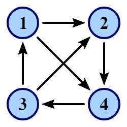
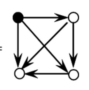
1
2
4
3
Transitive Tournament
Tournament: complete directed graph
Transitive tournament: acyclic tournament
\(v(n):\) Largest integer such that every tournament on \(n\) nodes contains a transitive subtournament on \(v(n)\) nodes.
\(\lfloor \log n \rfloor \leq \) \(v(n) \leq 1 + \lfloor 2\log n \rfloor\)
Counting
\(v(n) \leq 1 + \lfloor 2\log n \rfloor\)
\(v:= 2 + \lfloor 2\log n \rfloor\)
\(A:\) subset of \(n\) vertices of size \(v\)
\(\sigma:\) permutation on \([v]\)
\(\Gamma_{A,\sigma}:\) the set of \(n\)- vertex tournaments where \(A\) is a subtournament of it with "order" \(\sigma\)
We count the number \(d(\Gamma')\) of \(n\)- vertex tournaments with a transitive subtournament of size \(v\)
\(d(\Gamma') \leq \sum_A \sum_\sigma d(\Gamma_{A,\sigma}) = C^n_v v! 2^{C^n_2-C^v_2} < 2^{C^n_2}\)
\( (C^n_v v! < n^v \leq 2^{C^v_2})\)
Probabilistic Method
\(v(n) \leq 1 + \lfloor 2\log n \rfloor\)
\(v:= 2 + \lfloor 2\log n \rfloor\)
\(A:\) subset of \(n\) vertices of size \(v\)
\(\sigma:\) permutation on \([v]\)
Let \(T\) be the random variable uniformly distributed over all \(n\)-vertex tournaments.
We calculate the probability \(P(T\in \Gamma')\).
\(P(T\in \Gamma') \leq \sum_A \sum_\sigma P(T \in \Gamma_{A,\sigma}) = C^n_v v! 2^{-C^v_2} < 1\)
\( (C^n_v v! < n^v \leq 2^{C^v_2})\)
Incompressibility Method
\(v(n) \leq 1 + \lfloor 2\log n \rfloor\)
If \(v(n)\) is too large, then we can effectively compress every \(n\)-vertex tournament.
However, by the incompressibility method, there is some tournament \(T'\), where \(C(T'|n,p) \geq n(n-1)/2\).
(\(p\) is some decoding program)
For every tournament \(T\) of size \(n\), we can describe it by \(v(n) \lfloor \log n \rfloor+ n(n-1)/2 - v(n)(v(n)-1)/2\) bits.
Thus \(v(n) \lfloor \log n \rfloor - v(n)(v(n)-1)/2 \geq 0\), and
\(v(n) \leq 2 \lfloor \log n\rfloor + 1\).
?
Last Example:
Regular Languages
Regular Language
a language accepted by some DFA
a language decided by some constant-memory one-pass algorithm.
\(\iff\)
Regular Language
a language accepted by some DFA
a language decided by some constant-memory one-pass algorithm.
\(\iff\)
e.g. \(L = \{0^*1\}=\{1,01,001,0001,...\}\)
How to prove that a language is regular?
How to prove that a language is regular?
Construct a DFA/constant-memory one-pass algorithm for it.
How to prove that a language is regular?
Construct a DFA/constant-memory one-pass algorithm for it.
How to prove that a language is non-regular?
Pumping Lemma
Pumping Lemma
Might not be easy to use.
Not characterizing.
Example: Another possible way
Is \(L = \{0^k 1^k | k \geq 1\}\) a regular language?
Example: Another possible way
Is \(L = \{0^k 1^k | k \geq 1\}\) a regular language?
Suppose \(L\) is accepted by some DFA \(A\). Then we can recover \(k\) from \(A\) and \(q\), the state of \(A\) after processing \(0^k\). Thus for all \(k\geq 1\), \(C(k) = O(1)\).
KC-Regularity
Suppose \(L\) is regular, and \(L_x := \{y|xy \in L \}\). If \(y\) is the \(n\)-th string in \(L_x\), then \(C(y) \leq C(n) + O(1)\).
KC-Regularity
Suppose \(L\) is regular, and \(L_x := \{y|xy \in L \}\). If \(y\) is the \(n\)-th string in \(L_x\), then \(C(y) \leq C(n) + O(1)\).
*What does "the \(n\)-th string" mean?
More Examples
Is \(L := \{1^p |p\text{ is prime}\}\) a regular language?
Is \(L := \{x \bar x \}\) a regular language?
Regular KC-Characterization
In fact, we have
\(L\) is regular
For all \(x,n\), if \(y\) is the \(n\)-th string in \(L_x\), then \(C(y) \leq C(n) + O(1)\).
\(\Leftrightarrow\)
Thus, (in theory), we can also prove regularity!
Takeaways?
1. What is Kolmogorov complexity?
The Kolmogorov complexuty of a string (or number or sequence) is the minimum number of bits it can be compressed to.
2. What is the incompressibility method?
If an object satisfies some property, it can be efficiently compressed, but not everything can be efficiently compressed.
Some Questions
1. Alice and Bob are playing the number guessing game. Alice chooses some \(x \in [n]\), and Bob can ask her yes/no questions. If Alice can lie once, what is the minimum number \(c\) where Bob can always guess the right answer after asking \(c\) questions?
4. Why is computability important?
5. Ask a question!
3. Prove any (nontrivial?) statement you like via the incompressibility method.
2. What are the differences between counting, the probabilistic method, and the incompressibility method?
References
[1] Wikipedia contributors. (2023, March 5). Incompressibility method. In Wikipedia, The Free Encyclopedia. Retrieved 15:03, August 27, 2023, from https://en.wikipedia.org/w/index.php?title=Incompressibility_method&oldid=1143081380
[2] Wikipedia contributors. (2023, August 22). Kolmogorov complexity. In Wikipedia, The Free Encyclopedia. Retrieved 15:03, August 27, 2023, from https://en.wikipedia.org/w/index.php?title=Kolmogorov_complexity&oldid=1171617849
[3] Ming Li , Paul Vitányi. An Introduction to Kolmogorov Complexity and Its Applications, 2008.
A Little Bit of Computational Complexity
By Zi-Hong Xiao
A Little Bit of Computational Complexity
APCS Camp 資料結構


