Machine Learning in Intelligent Transportation
Session 2: Percepotron
Ahmad Haj Mosa
PwC Austria & Alpen Adria Universität Klagenfurt
Klagenfurt 2021

Machine Learning Tasks
1. Regression
Machine learning task are categorized by the target of the studies problems as follows:
is the problem of identifying the relationship (mathematical model) among different variables
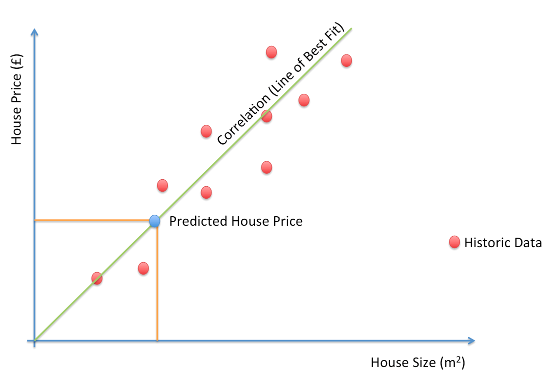
Linear Regression
A liner modeling of the relation between two or more variables
Text
y=\omega_1x+\omega_0
x
y
error
\( \omega_1 \) , \( \omega_0 \) are the weights
\( x \) is the independent variable (input/feature)
\( y \) is the dependent variable (decision/output)
Linear Regression Training
The training target of a linear regression is to find the optimum weights \( \omega_1 \) , \( \omega_0 \) that minimize the mean square error \( mse \)
Text
y=\omega_1x+\omega_0
x
y
error
p(x_0,y_0)
p(x_1,y_1)
p(x_2,y_2)
p(x_4,y_4)
p(x_5,y_5)
MSE=\frac{1}{n}\sum_{i=0}^{5}(y_i-\hat{y_{i}})^2
Gradient Descent
The training target of a linear regression is to find the optimum weights \( \omega_1 \) , \( \omega_0 \) that minimize the mean square error \( mse \)
MSE=\frac{1}{n}\sum_{i=0}^{5}(y_i-\hat{y_{i}})^2
Text
Text
\omega
MSE
Gradient Descent
The training target of a linear regression is to find the optimum weights \( \omega_1 \) , \( \omega_0 \) that minimize the mean square error \( mse \)
J=\frac{1}{n}\sum_{i=0}^{5}(y_i-\hat{y_{i}})^2
Text
\omega
J
\omega_{t+1}=\omega_{t}-\rho \frac{\partial J}{\partial \omega}
\( \ \frac{\partial J}{\partial \omega} \) is the gradient
\omega_{t=0}
\omega_{t=1}
\frac{\partial J}{\partial \omega} \simeq \frac{J_{t=1}-J_{t=0}}{1}<0
\frac{\partial J}{\partial \omega} \simeq \frac{J_{t=1}-J_{t=0}}{1}>0
\( \ \rho \) is the learning rate. Large \(\rho \) large steps
Gradient Descent
The training target of a linear regression is to find the optimum weights \( \omega_1 \) , \( \omega_0 \) that minimize the mean square error \( mse \)
J=\frac{1}{n}\sum_{i=0}^{5}(y_i-\hat{y_{i}})^2
\omega_{t+1}=\omega_{t}-\rho \frac{\partial J}{\partial \omega}
\( \ \frac{\partial J}{\partial \omega} \) is the gradient
\( \ \rho \) is the learning rate. Large \(\rho \) large steps
def gradient_descent(alpha, x, y, ep=0.0001, max_iter=10000):
    converged = False
    iter = 0
    m = x.shape[0] # number of samples

    # initial theta
    w0 = np.random.random(x.shape[1])
    w1 = np.random.random(x.shape[1])

    # total error, J(theta)
    J = sum([(t0 + t1*x[i] - y[i])**2 for i in range(m)])

    # Iterate Loop
    while not converged:
        # for each training sample, compute the gradient (d/d_theta j(theta))
        grad0 = 1.0/m * sum([(w0 + w1*x[i] - y[i]) for i in range(m)])
        grad1 = 1.0/m * sum([(w0 + w1*x[i] - y[i])*x[i] for i in range(m)])

        # update the theta_temp
        temp0 = w0 - alpha * grad0
        temp1 = w1 - alpha * grad1

        # update theta
        w0 = temp0
        w1 = temp1

        # mean squared error
        e = sum( [ (w0 + w1*x[i] - y[i])**2 for i in range(m)] )

        if abs(J-e) <= ep:
            print 'Converged, iterations: ', iter, '!!!'
            converged = True

        J = e   # update error
        iter += 1  # update iter

        if iter == max_iter:
            print 'Max interactions exceeded!'
            converged = True

    return w0,w1
y=\omega_1x+\omega_0
Machine Learning Tasks
1. Classification
Machine learning task are categorized by the target of the studies problems as follows:
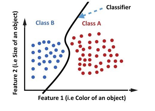
is the problem of identifying to which of a set of categories (sub-populations) a new observation
Linear Classifier
Text
x_2=\omega_1x_1+\omega_0
x_{1}
x_{2}
g(X)=W^TX
W=[\omega_1,\omega_2 ]^T
X=[x_1,x_2 ]^T
g(X)=0
g(X)>0
g(X)<0
From a linear Classifier to Neuron Models
Text
\omega^Tx
TH
y
y=f(\omega,x,T)
y= { 1 \text{ }\text{ }\text{ if } \text{ } \text{ } \text{ } \text{ } } \omega^Tx>TH
y= {0 \text{ }\text{ }\text{ if } \text{ } \text{ } \text{ } \text{ } } \omega^Tx<=TH
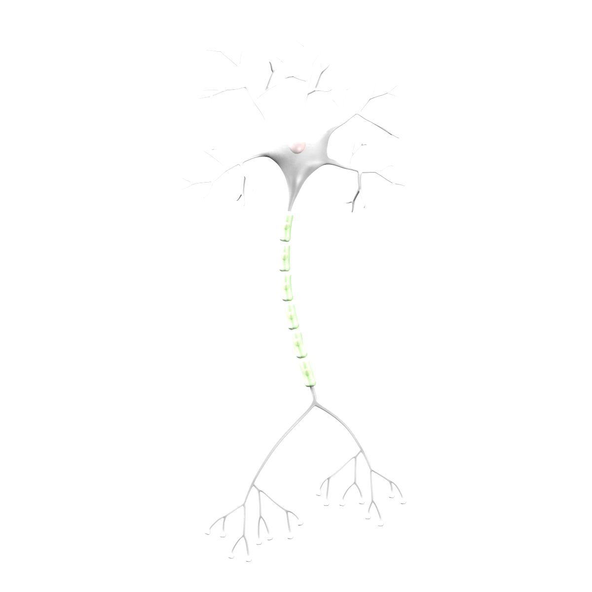
Dendrites
Axons
Cell body
\( x_1 \)
\( x_2 \)
\( y \)
Text
\( \omega= [\omega_1,\omega_2 ]^T \)
\( x=[x_1,x_2 ]^T \)
\( w_1 \)
\( w_2 \)
From a Neuron Model to Logistic Classification
Text
\omega^Tx
TH
y
y=f(\omega,x,T)
y= { 1 \text{ }\text{ }\text{ if } \text{ } \text{ } \text{ } \text{ } } \omega^Tx - TH >0
y= {0 \text{ }\text{ }\text{ if } \text{ } \text{ } \text{ } \text{ } } \omega^Tx - TH <=0
Dendrites
Axons
Cell body
\( x_1 \)
\( x_2 \)
\( y \)
\( w_1 \)
\( w_2 \)
y= { 1 \text{ }\text{ }\text{ if } \text{ } \text{ } \text{ } \text{ } } \omega^Tx - \omega_0 >0
y= {0 \text{ }\text{ }\text{ if } \text{ } \text{ } \text{ } \text{ } } \omega^Tx - \omega_0 <=0
y= { 1 \text{ }\text{ }\text{ if } \text{ } \text{ } \text{ } \text{ } } \omega^Tx>0
y= {0 \text{ }\text{ }\text{ if } \text{ } \text{ } \text{ } \text{ } } \omega^Tx<=0
\( \omega= [\omega_1,\omega_2 ,\omega_0]^T \)
\( x=[x_1,x_2,-1 ]^T \)
Text
\( -1 \)
\( w_0 \)
The Perceptron Algorithm
The perceptron algorithm is an optimization method to compute the unknown weights \( w^T \)
- Assume we have classification problem with two classes \( c_1, c_2 \)
c_1{ \text{ }\text{ }\text{ if } \text{ } \text{ } \text{ } \text{ } } \omega^Tx>0
c_2{ \text{ }\text{ }\text{ if } \text{ } \text{ } \text{ } \text{ } } \omega^Tx<0
- The perceptron cost is given by:
J(\omega)= \sum_{x \epsilon Y}(\delta_xw^Tx)
- Where \( Y \) is the subset of the samples, which are misclassified by the classifier
\omega(t+1)=\omega(t)-\rho_t\frac{\partial J}{\partial \omega}
\frac{\partial J}{\partial \omega}=\sum_{x \epsilon Y}(\delta_xx)
\omega(t+1)=\omega(t)-\rho_t\sum_{x \epsilon Y}(\delta_xx)
- The variable \( \delta_x \) is chosen so that \( \delta_x =-1 \) if \( x \epsilon c_1 \) and \( \delta_x =1 \) if \( x \epsilon c_2 \)
The Perceptron Algorithm
The perceptron algorithm is an optimization method to compute the unknown weights \( w^T \)
- Choose \( \omega_0 \) randomly
- Choose \( \rho_0 \)
- \( t=0 \)
- Repeat :
- \( Y = \phi \)
- For \(i=1\) to \(N\) :
- If \( \delta_{x_i}\omega(t)^Tx_i \geq 0\) then \( Y=Y \cup {x_i} \)
- End {For}
- \( \omega(t+1) = \omega(t) - \rho \sum_{x \epsilon Y}\delta_{x} x \)
- \(t=t+1\)
- Until \(Y= \phi \)
J(\omega)= \sum_{x \epsilon Y}(\delta_xw^Tx)
\omega(t+1)=\omega(t)-\rho_t\sum_{x \epsilon Y}(\delta_xx)
Nonlinear Classifiers
For nonlinear separable problems a single neuron/line model in not enough
Logical OR Modeling: linear classifier?
| OR | Class | ||
|---|---|---|---|
| 0
|
0 | 0 | B |
| 0 | 1 | 1 | A |
| 1 | 0 | 1 | A |
| 1 | 1 | 1 | A |
x_1
x_2
Text
x_{1}
x_2
A
A
A
B
\omega^Tx
\( y \)
\( w_2 =1 \)
Text
\( -1/2 \)
\( w_0 \)
\( w_1 =1 \)
x_{1}
x_2
\( y =x_1 +x_2 -0.5\)
Logical AND Modeling: linear classifier?
| AND | Class | ||
|---|---|---|---|
| 0
|
0 | 0 | B |
| 0 | 1 | 0 | B |
| 1 | 0 | 0 | B |
| 1 | 1 | 1 | A |
x_1
x_2
Text
x_{1}
x_2
A
B
B
B
\omega^Tx
\( y \)
\( w_2 =1 \)
Text
\( -3/2 \)
\( w_0 \)
\( w_1 =1 \)
x_{1}
x_2
\( y =x_1 +x_2 -3/2\)
Logical XOR Modeling: linear classifier?
| XOR
|
Class | ||
|---|---|---|---|
| 0
|
0 | 0 | B |
| 0 | 1 | 1
|
A
|
| 1 | 0 | 1
|
A
|
| 1 | 1 | 0
|
A
|
x_1
x_2
Text
x_{1}
x_2
A
B
B
\omega^Tx
\( y \)
\( -3/2 \)
\( 1 \)
x_{1}
x_2
\( y =(x_1 +x_2 -1/2)+2(x_1 +x_2 -3/2)- 1/2\)
A
Text
\( 1 \)
\( 1 \)
\( 1 \)
\( -1/2 \)
\( -1/2 \)
\( 2 \)
\( 1 \)
Neural Networks: topological representation
Topology is one field of mathematics that can be used to understand how neural networks work
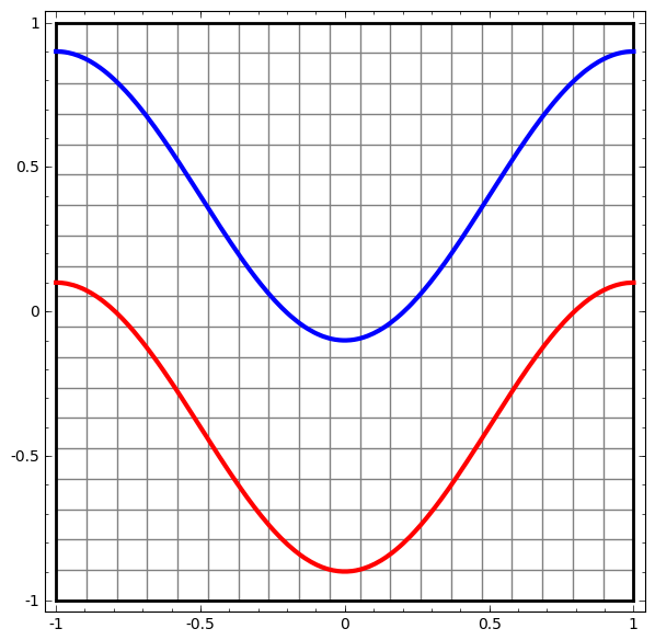
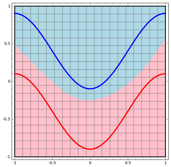
- A simple NN topology example: a very simple dataset, two curves on a plane. The network will learn to classify points as belonging to one or the other.
Text
Neural Networks: topological representation
Topology is one field of mathematics that can be used to understand how neural networks work
- The two regions can only be separated by a nonlinear curve
Text
Neural Networks: topological representation
Topology is one field of mathematics that can be used to understand how neural networks work
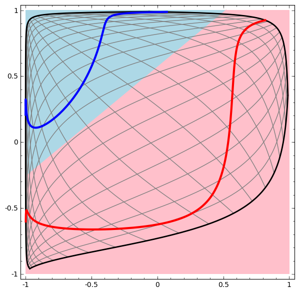
- With each layer, the network transforms the data, creating a new representation
- When we get to the final representation, the network will just draw a line through the data (or, in higher dimensions, a hyperplane).
Session 2: Linear and Logistic Regression
By ahmadadiga


