Embracing Noise in Neural Models

Accounting for replication noise in model selection

Alexandre René

rene@netsci.rwth-aachen.de

SSC annual meeting • Session on Noise in Neural Systems
1 Jun 2026 • Hamilton

Neural Models are always Misspecified

We don’t know everything
Even if we did, we don’t want to model everything

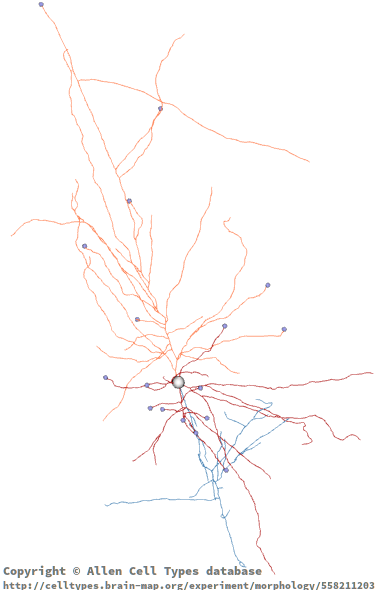
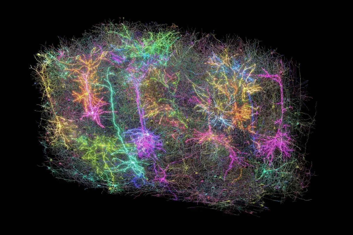
1,000 neurons of mouse brain © Allen institute

Fully mechanistic model
aka “bottom-up”

Effective model

Physics-inspired neural network (PINN)

Neural-network w/ interpretable dimensions

Black box
neural network

Interpretability

Flexibility of construction

Data requirements

Different Approaches to Dealing with Misspecificaton

Effective model

Neural-network w/ interpretable dimensions

Different Approaches to Dealing with Misspecificaton

Effective models

Mechanistic model derived under assumption of homogeneous populations.
- Deterministic: \(A(t) = f_{\mathcal{M}_θ}\bigl(I(t); S_t\bigr)\)
- Probabilistic: \(A(t) \sim P\bigl(A(t) \mid I(t); \mathcal{M}_θ \bigr) \)
Mechanistic equations provide a
model-informed loss functional: the log likelihood
- Given observations \(\{I(t_i), A(t_i)\}_{i=1, 2, \dotsc}\), solve
- In contrast to e.g. least-squares, loss values away from minimum remain comparable
A data-driven approach to effective models:
heterogeneous pops ⟼ homogeneous pops w/ effective params

(∞-pops)

(finite-pops)

pop activity

input

internal state

model

(René et al,, Neural Computations 2020)

\(i\) :

sample index

\hat{θ} = \argmin_θ - \sum_i \log P\bigl(A(t_i) \mid I(t_i); \mathcal{M}_θ \bigr)

more robust inference, better generalization

Different Approaches to Dealing with Misspecificaton

Effective models

Mechanistic model: \(A(t) \sim P\bigl(A(t) \mid I(t); \mathcal{M}_θ \bigr) \)
Model-informed loss functional: the log likelihood
A data-driven approach to effective models:
heterogeneous pops ⟼ homogeneous pops w/ effective params

(finite-pops)

(René et al,, Neural Computations 2020)

\hat{θ} = \argmin_θ - \sum_i \log P\bigl(A(t_i) \mid I(t_i); \mathcal{M}_θ \bigr)

more robust inference, better generalization

Highly nonlinear model ⇒ multitude of solutions

Different Approaches to Dealing with Misspecificaton

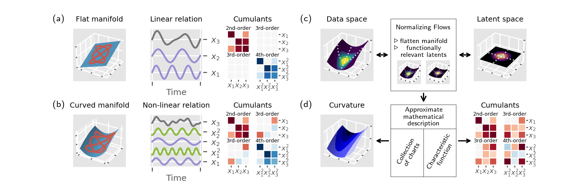
Neural networks with interpretable dimensions

(Bouss et al., PRX Life 2026)

If we don’t have a mechanistic model, we may still learn the data distribution.
If we are very lucky, data may
- lie on a flat manifold
- and be Gaussian

\Biggr\}

then we can use PCA to learn the data distribution

Different Approaches to Dealing with Misspecificaton

Neural networks with interpretable dimensions

(Bouss et al., PRX Life 2026)

If we don’t have a mechanistic model, we may still learn the data distribution.
If we are very lucky, data may
- lie on a flat manifold
- and be Gaussian
An invertible neural network learns a diffeomorphism between the data dimensions and latent dimensions with a flat Gaussian
- This way it can learn non-parametric distributions on nonlinear manifolds
- Bijective map preserves interpretability of latent space.

\Biggr\}

then we can use PCA to learn the data distribution

Different Approaches to Dealing with Misspecificaton

Neural networks with interpretable dimensions

(Bouss et al., PRX Life 2026)

If we don’t have a mechanistic model, we may still learn the data distribution.
An invertible neural network (INN) learns a diffeomorphism between the data dimensions and latent dimensions
- ⇒ non-parametric distributions on nonlinear manifolds
- Bijective map preserves interpretability of latent space.
We add a penalty to encourage a low-dimensional description
- If data > noise, this separate data and noise dimensions

\mathcal{L}(θ) = - \frac{1}{L} \frac{1}{|\mathcal{D}|} \sum_{y \in \mathcal{D}} \log \hat{p}_{|\mathcal{D},θ}(y) + γ \frac{1}{d_r} \sum_{l=1}^{d_r} R_l(θ)

log likelihood given by INN

Reconstruction accuracy keeping only \(l\) dimensions
→ lower dimensions show up in more terms

→ encourage low dimensions to be efficienc

Different Approaches to Dealing with Misspecificaton

Neural networks with interpretable dimensions

(Bouss et al., PRX Life 2026)

If we don’t have a mechanistic model, we may still learn the data distribution.
An invertible neural network (INN) learns a diffeomorphism between the data dimensions and latent dimensions
- ⇒ non-parametric distributions on nonlinear manifolds
- Bijective map preserves interpretability of latent space.
We add a penalty to encourage a low-dimensional description
- If data > noise, this separate data and noise dimensions
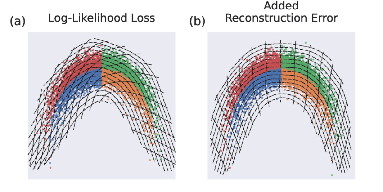
Applied to electrophysiological data (Utah array)

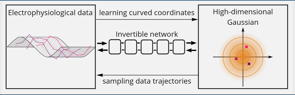
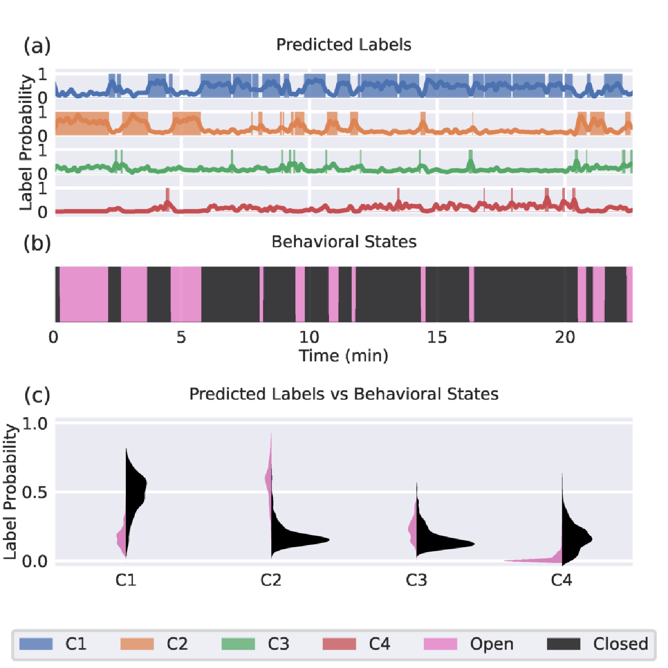
States

Latent component strongly correlated w/ state

Again, INN is a highly nonlinear model

⇒ multitude of solutions

Facing the Music

of Multiple Models

Usual scientific workflow

Anecdotal

observations

<MEDIA>@s3.amazonaws.com

What we want in a Selection Criterion

Usual scientific workflow

Conceive theory

Conceive experiment

Accumulate data

Compare

Make prediction

New experiment?

Assumptions

Symmetry

Conservation

Exchangeability

Anecdotal

observations

<MEDIA>@s3.amazonaws.com

Validate/falsify

In science the goal is induction:
to find a general model from particular experiments
Scientific tradition has developed a way to do this:
evaluate predictions on replication experiments.

What we want in a Selection Criterion

Select the model which is “best” on replications.

Scientific wisdom:

Machine learning wisdom:

“best” → lowest (empirical) risk

Prinz et al., Nat Neurosci (2004)

René, Pyloric simulator, PyPI (2025)

C_a \frac{dV}{dt} = \;\;\sum_{\mathclap{\text{ion channels}}}\; \bar{g}_i m_i[V]^p h_i[V] (V - E_i)

\begin{aligned} \mathcal{B}_{\mathrm{RJ}}(λ; T) &= \frac{2 c k_B T}{λ^4} \\ \mathcal{B}_\mathrm{P}(λ; T) &= \frac{2 h c^2}{λ^5} \frac{1}{\exp\left( \frac{hc}{λ k_B T} \right) - 1} \end{aligned}

Two model examples

Radiance of a Black Body

Neurons of the Crustacean Pyloric Circuit

Fitting parameters

→ Distinct local solutions

Two model candidates
Models ↔

Different equations
Different parameters

Two model candidates
Models ↔

Same equations
Different parameters

Rayleigh-Jeans

Planck

Standard statistical criteria

EMD criterion

Prinz et al., Nat Neurosci (2004)

René, Pyloric simulator, PyPI (2025)

C_a \frac{dV}{dt} = \;\;\sum_{\mathclap{\text{ion channels}}}\; \bar{g}_i m_i[V]^p h_i[V] (V - E_i)

\begin{aligned} \mathcal{B}_{\mathrm{RJ}}(λ; T) &= \frac{2 c k_B T}{λ^4} \\ \mathcal{B}_\mathrm{P}(λ; T) &= \frac{2 h c^2}{λ^5} \frac{1}{\exp\left( \frac{hc}{λ k_B T} \right) - 1} \end{aligned}

Two model examples

Radiance of a Black Body

Neurons of the Crustacean Pyloric Circuit

Two model candidates
Models ↔

Different equations
Different parameters

Two model candidates
Models ↔

Same equations
Different parameters

Rayleigh-Jeans

Planck

\left\{\begin{aligned} &\mathcal{M}_A \\ &\;\;\;\vdots \\ &\mathcal{M}_Z \end{aligned}\right\}

\left\{\begin{aligned} &\mathcal{M}_C \\ &\mathcal{M}_E \\ &\mathcal{M}_P \end{aligned}\right\}

Goal

selection
criterion

Only reject if enough evidence
⤷No forced choiced

We will use risk: \(\mathbb{E}_{\mathcal{M}_{\mathrm{true}}}[Q]\) to rank models

Some loss

\(θ_A\) subsumed into \(\mathcal{M}_A\)

The problem with Forced Choice

Data

Empirical Risk

Not all comparisons should be conclusive

Result is not consistent across replications

Intuition: More predictive accuracy ⇒ More reliable comparison

Why? If we know a source of variable, we can:

account for it in the model
control for it in the experiment

EMD assumption: Model discrepancies are due to unknown variability

Unknown sources of variability may change across experiments

Empirical risk accounts for predictive performance and non-stationary replications (aka generalization)
(“consistency”)
But still a forced choice: no notion of uncertainty
We are going to construct a criterion which bootstraps epistemic uncertainty from prediction discrepancies:
Empirical Modelling Discrepancy (EMD)

Ranking models based on empirical risk

\(R\): Risk
(lower is better)

Are these differences in risk all meaningful?

Data

Pointwise loss

(Empirical) risk

\((x_i, y_i) \sim \mathcal{D}_{\mathrm{true}} \)

\(Q(x_i, y_i \mid \mathcal{M}_A) \to \mathbb{R}\)

\(\mathbb{E}\bigl[Q(x_i, y_i \mid \mathcal{M}_A) \bigr] \approx \frac{1}{L} \;\sum\limits_{\mathclap{\qquad(x_i, y_i) \sim \mathcal{D}_{\mathrm{true}}}}\;\; Q(x_i, y_i \mid \mathcal{M}_A) \)

NB: \(θ\) subsumed into \(\mathcal{M}_a\)

We assume to have

\(\bigl\{\mathcal{M}_A, \mathcal{M}_B, \dotsc \bigr\}\)
each defining \(p(x_i, y_i \mid \mathcal{M}_a) \)
\(Q: \mathcal{X} \times \mathcal{Y} \to \mathbb{R} \)
ability to sample \(\mathcal{M}_{\mathrm{true}}\)

Empirical risk accounts for predictive performance and non-stationary replications (aka generalization)
(“consistency”)
But still a forced choice: no notion of uncertainty
We are going to construct a criterion which bootstraps epistemic uncertainty from prediction discrepancies:
Empirical Modelling Discrepancy (EMD)

Ranking models based on empirical risk

\(R\): Risk
(lower is better)

Are these differences in risk all meaningful?

Data

Pointwise loss

(Empirical) risk

\((x_i, y_i) \sim \mathcal{D}_{\mathrm{true}} \)

\(Q(x_i, y_i \mid \mathcal{M}_A) \to \mathbb{R}\)

\(\mathbb{E}\bigl[Q(x_i, y_i \mid \mathcal{M}_A) \bigr] \approx \frac{1}{L} \;\sum\limits_{\mathclap{\qquad(x_i, y_i) \sim \mathcal{D}_{\mathrm{true}}}}\;\; Q(x_i, y_i \mid \mathcal{M}_A) \)

NB: \(θ\) subsumed into \(\mathcal{M}_a\)

We assume to have

\(\bigl\{\mathcal{M}_A, \mathcal{M}_B, \dotsc \bigr\}\)
each defining \(p(x_i, y_i \mid \mathcal{M}_a) \)
\(Q: \mathcal{X} \times \mathcal{Y} \to \mathbb{R} \)
ability to sample \(\mathcal{M}_{\mathrm{true}}\)

How do we measure this?

And turn it into this?

Discrepancy

Model ↔ Quantile Function

For purposes of calculating risk, we can reduce any model to \(q(Φ)\) without loss of information

\begin{aligned} R_A &:= \mathbb{E}_{\mathcal{M}_\mathrm{true}}\bigl[Q(x_i, y_i \mid \mathcal{M}_A) \bigr] \\ &\;= \int_{\mathcal{X}\times\mathcal{Y}} \hspace{-18mu} dxdy\, p(x,y \mid \mathcal{M}_{\mathrm{true}}) \; Q(x, y \mid \mathcal{M}_A) \\ &\;= \int_{-\infty}^\infty \hspace{-12mu} dq \int_{\substack{\\\!\!\!\!\!\mathcal{X}\times\mathcal{Y}\\\!\!\!Q(x,y)=q}} \hspace{-32mu} dxdy\,p(x,y \mid \mathcal{M}_{\mathrm{true}}) \; Q(x, y \mid \mathcal{M}_A) \\ &\;= \int_{-\infty}^\infty \hspace{-6mu} dq \;q\; p(q \mid \mathcal{M}_\mathrm{true}, \mathcal{M}_A) \\ &\;= \int_{-\infty}^\infty \hspace{-6mu} dq \;q(Φ \mid \mathcal{M}_\mathrm{true}, \mathcal{M}_A) \frac{d}{dq} Φ \\ R_A &\;= \int_{0}^{1} q(Φ\mid \mathcal{M}_\mathrm{true}, \mathcal{M}_A) dΦ \end{aligned}

\begin{aligned} \vphantom{Φ(q \mid \mathcal{M}_{\mathrm{true}}, \mathcal{M}_A)} Φ(q \mid \dots) &= \int_{\substack{\\\!\!\!\!\!\mathcal{X}\times\mathcal{Y}\\\!\!\!Q(x,y){\color{blue} \bm{\leq}} q}} \hspace{-32mu} dxdy\; Q(x, y \mid \mathcal{M}_A) p(x,y \mid \mathcal{M}_{\mathrm{true}}) \\[5ex] &\approx \frac{1}{\lvert \mathcal{D} \rvert} \sum_{\mathcal{D}} \bigl[ Q(x,y) \leq q \bigr] \end{aligned}

R_A \;= \int_{0}^{1} q(Φ \mid \mathcal{M}_\mathrm{true}, \mathcal{M}_A) dΦ \quad {\color{grey} \approx \frac{1}{\lvert \mathcal{D} \rvert} \sum_{(x,y)\in\mathcal{D}} Q(x,y \mid \mathcal{M}_A)}

tldr: Use Fubini’s theorem to rewrite risk integral

Model ↔ Quantile Function

For purposes of calculating risk, we can reduce any model to \(q(Φ)\) without loss of information

EMD assumption (reframed): Candidate models represent that part of the experiment which we understand and control across replications

We can estimate \(R_A\) in two different ways:

\tilde{R}_A = \int_{\mathcal{X}\times\mathcal{Y}} \hspace{-18mu} dxdy\; Q(x, y \mid {\color{blue} \mathcal{M}_A}) p(x,y \mid {\color{blue} \mathcal{M}_A}) \\

R_A^* = \int_{\mathcal{X}\times\mathcal{Y}} \hspace{-18mu} dxdy\; Q(x, y \mid {\color{blue} \mathcal{M}_A}) p(x,y \mid {\color{blue} \mathcal{M}_{\mathrm{true}}}) \\

Mixed \(q_A^*\)

Synth \(\tilde{q}_A\)

Repeat for each \(\mathcal{M}\)

Stochastic Processes on Quantile Functions

Desiderata

Any process \(\mathcal{Q}\) should be

monotone
integrable
non-accumulating

\mathbb{E}\bigl[ \lvert q(Φ + ΔΦ) - q(Φ) \rvert \bigr] \lesssim C \, ΔΦ

There is no way to coax a Wiener process to yield what we need

Variance must not depend on \(Φ\), only on \(δ^{\mathrm{EMD}}(Φ)\)

\(\hat{q}\) should be “centered” on \(q^*\)
The “variability” of \(\hat{q}\) should be proportional to \(\color{#FF7b00} δ^{\mathrm{EMD}}\)

\begin{aligned} &\tilde{q}(Φ+ΔΦ) \\ &\quad= \tilde{q}(Φ) + \mathcal{N}\bigl[q^*(Φ+ΔΦ) - q^*(Φ), c(δ^{\mathrm{EMD}})^2\bigr] \end{aligned}

Hierarchical Beta Process on Quantile Functions

Instead of accumulating increments left-to-right, we successively refine the interval

We draw increment pairs, under the constraint

\(Δq_{ΔΦ}(Φ) \stackrel{!}{=} Δq_{ΔΦ/2}(Φ) + Δq_{ΔΦ/2}(Φ+ΔΦ/2)\)

\Rightarrow

We need a compositional distribution

Mateu-Figueras et al., Distributions on the Simplex Revisited, 2021

The simplest 2-D compositional distributon is the beta distribution

\begin{aligned} &\tilde{q}(Φ+ΔΦ) \\ &\quad= \tilde{q}(Φ) + \mathcal{N}\bigl[q^*(Φ+ΔΦ) - q^*(Φ), c(δ^{\mathrm{EMD}})^2\bigr] \end{aligned}

ΔΦ = 2^{-1}

ΔΦ = 2^{-2}

ΔΦ = 2^{-3}

ΔΦ = 2^0

Hierarchical Beta Process on Quantile Functions

We draw increment pairs, under the constraint

\(Δq_{ΔΦ}(Φ) \stackrel{!}{=} Δq_{ΔΦ/2}(Φ) + Δq_{ΔΦ/2}(Φ+ΔΦ/2)\)

Beta

\begin{alignedat}{7} x &\sim \mathop{\mathrm{Beta}} &&\Rightarrow\; & p(x) &\propto x^α (1 - x)^β &&\,,& \quad x &\in [0, 1] \\ \phantom{x_1, x_2}&\phantom{\sim \mathop{\mathrm{Beta}}} &&\phantom{\Rightarrow\;} & \phantom{p(x_1,x_2)} &\phantom{\propto x_1^α\;\; x_2^β} &&\phantom{\,,}& \phantom{\quad x_1,x_2} &\phantom{\in [0, 1], \, x_1 + x_2 \stackrel{!}{=} 1} \end{alignedat}

Compositional form

Desiderata

monotone
integrable
non-accumulating

\left.\begin{aligned} \\[4ex] \end{aligned}\right\}

By construction

\(\hat{q}\) should be “centered” on \(q^*\)

\left.\begin{aligned} \\[4ex] \end{aligned}\right\}

Determine \(α\) and \(β\)

\begin{alignedat}{7} \phantom{x} &\phantom{\sim \mathop{\mathrm{Beta}}} &&\phantom{\Rightarrow\;} & \phantom{p(x)} &\phantom{\propto x^α (1 - x)^β} &&\,\phantom{,}& \quad \phantom{x} &\phantom{\in [0, 1]} \\ x_1, x_2&\sim \mathop{\mathrm{Beta}} &&\Rightarrow\; & p(x_1,x_2) &\propto x_1^α\;\; x_2^β &&\,,& \quad x_1,x_2 &\in [0, 1], \, x_1 + x_2 \stackrel{!}{=} 1 \end{alignedat}

The “variability” of \(\hat{q}\) should be proportional to \(\color{#FF7b00} δ^{\mathrm{EMD}}\)

Hierarchical Beta Process on Quantile Functions

We draw increment pairs, under the constraint

\(Δq_{ΔΦ}(Φ) \stackrel{!}{=} Δq_{ΔΦ/2}(Φ) + Δq_{ΔΦ/2}(Φ+ΔΦ/2)\)

Beta

\(\hat{q}\) should be “centered” on \(q^*\)

The “variability” of \(\hat{q}\) should be proportional to \(\color{#FF7b00} δ^{\mathrm{EMD}}\)

Because of the constraint, mean and variance are not natural statistics for compositional distributions

Mateu-Figueras et al., Distributions on the Simplex Revisited, 2021

Instead it is better to use the center and metric variance

\mathbb{E}_a[(x_1, x_2)] = \frac{1}{e^{ψ(α)} + e^{ψ(β)}} \bigl(e^{ψ(α)}, e^{ψ(β)}\bigr)

\mathop{\mathrm{Mvar}}[(x_1, x_2)] = \frac{1}{2} \bigl(ψ_1(α) + ψ_1(β)\bigr)

Two equations ⇒ Solve for \(α\) and \(β\)

\frac{e^{ψ(α)}}{e^{ψ(β)}} \stackrel{!}{=} \frac{Δq_{ΔΦ}^*(Φ)}{Δq_{ΔΦ}^*(Φ+ΔΦ)}

\mathop{\mathrm{Mvar}}[(x_1, x_2)] \stackrel{!}{=} c\,δ^\mathrm{EMD}

Summary – Ideas

Our high-level goal is induction

→ High predictive accuracy on future replications

We use risk: \(\mathbb{E}_{\mathcal{M}_{\mathrm{true}}}[Q]\) to rank models

For purposes of calculating risk, we can reduce any model to \(q(Φ)\) without loss of information

Assumption: Candidate models represent that part of the experiment which we understand and control across replications

Hierarchical beta process: To obtain a non-accumulating process over quantile functions, we successively refine the interval

Ansatz: Model uncertainty proportional to \(δ^{\mathrm{EMD}}\)

R_A \;= \mathbb{E}_{\mathcal{M}_\mathrm{true}}\bigl[Q(x_i, y_i \mid \mathcal{M}_A) = \int_{0}^{1} dΦ(q \mid \mathcal{M}_\mathrm{true}, \mathcal{M}_A)

Better noise produces better models

→

There is a cost to over-simplifying noise, eg. w/ least squares

Summary – Procedure

Repeat for each \(\mathcal{M}\)

Calibration

Summary – Procedure

Repeat for each \(\mathcal{M}\)

Calibration

All of this can be automated

emdcmp on PyPI

from emdcmp import Bemd, make_empirical_risk, draw_R_samples

synth_ppfA = make_empirical_risk(lossA(modelA.generate(Lsynth)))
synth_ppfB = make_empirical_risk(lossB(modelB.generate(Lsynth)))
mixed_ppfA = make_empirical_risk(lossA(data))
mixed_ppfB = make_empirical_risk(lossB(data))

Bemd(mixed_ppfA, mixed_ppfB, synth_ppfA, synth_ppfB, c=c)

Thank You

Chair of Computational Network Science

(Prof. Michael Schaub)

netsci.rwth-aachen.de

Alexandre René
rene@netsci.rwth-aachen.de
www.arene.ca

Learning effective models

Cited papers

René, Longtin, Macke, Inference of a Mesoscopic Population Model from Population Spike Trains, Neural Computation (2020)

Learning invertible neural network

René, Longtin, Macke, Characterizing Neural Manifolds' Properties and Curvatures using Normalizing Flows, PRX Life (2026)

Epistemically-robust model selection

René, Longtin, Selecting fitted models under epistemic uncertainty using a stochastic process on quantile functions, Nature Communications (2025)

Extra slides

We can learn more, and more complex, models

Multiple LP candidates with similar responses

Prinz et al., Nat Neurosci (2004)

René, pyloric simulator, PyPI (2025)

C_a \frac{dV}{dt} = \;\;\sum_{\mathclap{\text{ion channels}}}\; \bar{g}_i m_i[V]^p h_i[V] (V - E_i)

8D Parameter sweep

… arguably too many models

t_k

t_{k-1}

t_{k-2}

…

\nabla_{\color{#3cb100} Θ}

René et al., Neural Comp (2020)

Back-propagation through time

Hierarchical Beta Process on Quantile Functions

A Qualitatively Different Criterion

Dataset size

“Strength” of evidence

BIC

Bayes factor

MDL

AIC

elpd

No
Partially —
vol(posterior)
No
No
No

No
Yes —
vol(posterior)
No
No
No

No
Yes — ability to fit arb. data
No
No
No

Partially — unbiased est.
No
No
No
No

Yes
No
No
No
No

EMD

High-level goal is induction
Objective is predictive accuracy
No model is perfect
The amount of data is undetermined

Considers generalization error
Penalizes model complexity
Allows for misspecified models
Allows for non-stationary replications
Bounded discriminability (as \(\lvert\mathcal{D}\rvert \to \infty\))

Yes
No
No
No
No

Calibration: Putting units on the proportionality

\bm{ δ^\mathrm{EMD} }

\mathop{\mathrm{Mvar}}[(x_1, x_2)] \stackrel{!}{=} {\color{1692ad} c} \,δ^\mathrm{EMD}

Converts discrepancy to metric variance
Context-dependent: chosen by
simulating experimental variations

Procedure

Use domain & problem knowledge to define “epistemic distributions” \(Ω\) over
- weak vs strong input
- data correlations
- temperature
- …
Simulate 1000’s of model comparisons for each tested value of \(c\)
Compare to the ground truth probabilities
Select a \(c\) which systematically underestimates selection confidence

B^\mathrm{EMD}_{AB} := P(R_A < R_B \mid c)

Use the fact that \(B^\mathrm{EMD}_{AB}\) are true probabilities:

B^\mathrm{epis}

Calibration: Putting units on the proportionality

\bm{ δ^\mathrm{EMD} }

Procedure

Use domain & problem knowledge to define “epistemic distributions” \(Ω\) over
- weak vs strong input
- data correlations
- temperature
- …
Simulate 1000’s of model comparisons for each tested value of \(c\)
Compare to the ground truth probabilities
Select a \(c\) which systematically underestimates selection confidence

B^\mathrm{EMD}_{AB} := P(R_A < R_B \mid c)

Use the fact that \(B^\mathrm{EMD}_{AB}\) are true probabilities:

(white region)

B^\mathrm{epis}

(true)

(theory)

What kind of robustness do we seek?

Variations

At a large scale, what kinds of variations do we want to account for?

In-distribution data
Out-of-distribution data
Model parameters

High-level

Paradigm

How do we define/quantify these variations and the selection objective?

Specific

Epistemic distribution (\(Ω\))
Data-generating process (\(\mathcal{M}_{\mathrm{true}}\))
Dataset (\(\mathcal{D}\))
Parameters (\(θ\))
Score function (\(R\))
Evaluate score on…

Properties

Higher-level assessment.
These follow from the choice of paradigm.

Functional

Considers generalization error
Penalizes model complexity
Allows for misspecified models
Allows for non-stationary replications
Bounded discriminability (as \(L \to \infty\))

Different criteria ↔ Different notions of robustness

Variations

Paradigm

Properties

In-distribution data
Out-of-distribution data
Model parameters

Epistemic distribution (\(Ω\))
Data-generating process (\(\mathcal{M}_{\mathrm{true}}\))
Dataset (\(\mathcal{D}\))
Parameters (\(θ\))
Score function (\(R\))
Evaluate score on…

Considers generalization error
Penalizes model complexity
Allows for misspecified models
Allows for non-stationary replications
Bounded discriminability (as \(L \to \infty\))

BIC

Bayes factor

ε_A = \int p(\mathcal{D}|θ,\mathcal{M}_A){\color{blue} π_A(θ) dθ}

MDL

AIC

elpd

\mathtt{COMP}(\mathcal{M}_A) = \int {\color{blue} \max_θ}\; p({\color{red} \mathcal{D}'}|\mathcal{M}_A({\color{blue} θ})) d{\color{red} D'}

\mathbb{E}_{{\color{blue} (x_i, y_i)} \sim \mathcal{M}_{\mathrm{true}}} [Q({\color{blue} x_i, y_i}; \mathcal{M}_A)]

2 Q({\color{red} \mathcal{D}_{\mathrm{train}}}; \mathcal{M}_A\bigl({\color{green} \hat{θ}}({\color{red} \mathcal{D}_{\mathrm{train}}})\bigr)) + k_A \cdot 2

2 Q\bigl({\color{red} \mathcal{D}_{\mathrm{train}}}; \mathcal{M}_A\bigl({\color{green} \hat{θ}}({\color{red} \mathcal{D}_{\mathrm{train}}})\bigr)\bigr) + k_A \lvert\mathcal{D}\rvert

Bayesian information criterion

aka model evidence

minimum description length

Akaike information criterion

expected log pointwise predictive density

\log ε_A - \log ε_B

p\bigl(\mathcal{D} \mid \mathcal{M}_A\bigl({\color{green} \hat{θ}}(\mathcal{D}_{\mathrm{train}})\bigr)\bigr)

Ignoring

model
vs
discrete params
vs
continuous params

See esp. “Holes in Bayesian Statistics”, Gelman, Yao, J. Phys. G (2020)

Different criteria ↔ Different notions of robustness

Variations

Paradigm

Properties

In-distribution data
Out-of-distribution data
Model parameters

Epistemic distribution (\(Ω\))
Data-generating process (\(\mathcal{M}_{\mathrm{true}}\))
Dataset (\(\mathcal{D}\))
Parameters (\(θ\))
Score function (\(R\))
Evaluate score on…

Considers generalization error
Penalizes model complexity
Allows for misspecified models
Allows for non-stationary replications
Bounded discriminability (as \(L \to \infty\))

BIC

Bayes factor

ε_A = \int p(\mathcal{D}|θ,\mathcal{M}_A)π_A(θ) dθ

MDL

AIC

elpd

N/A
N/A
Fixed \(\mathcal{D}_{\mathrm{rep}} \equiv \mathcal{D}_{\mathrm{obs}}\)
(\(θ\sim \text{prior}\))
Log likelihood
Training data, joint

N/A
N/A
Fixed \(\mathcal{D}_{\mathrm{rep}} \equiv \mathcal{D}_{\mathrm{obs}}\)
(\(θ\sim \text{prior}\))
Log likelihood
Training data, joint

No
Yes
Yes

Single \(Ω\):
\(\mathcal{M}_{\mathrm{true}} \sim Ω\)
\(\mathcal{D}_{\mathrm{rep}} \sim\) event space
Fit \(θ\) to \(\mathcal{D}_{\mathrm{rep}} \)
Log likelihood
Training data, joint

Yes
No
No

N/A
Fixed \(\mathcal{M}_{\mathrm{true}}\)
\(\mathcal{D}_{\mathrm{rep}} \sim \mathcal{M}_{\mathrm{true}}\)
Fit \(θ\) to \(\mathcal{D}_{\mathrm{rep}} \)
Log likelihood
Training data, joint

Yes
Yes
No

Single \(Ω\):
\(\mathcal{M}_{\mathrm{true}} \sim Ω\)
\(\mathcal{D}_{\mathrm{rep}} \sim \mathcal{M}_{\mathrm{true}}\)
Fit posterior to \(\mathcal{D}_{\mathrm{obs}} \)
Arbitrary functional
Test data, pointwise total

prior over models

posterior over params

\int {\color{blue} \max_θ}\; p({\color{red} \mathcal{D}'}|\mathcal{M}_A({\color{blue} θ})) d{\color{red} D'}

\mathbb{E}_{{\color{blue} (x_i, y_i)} \sim \mathcal{M}_{\mathrm{true}}} [Q({\color{blue} x_i, y_i}; \mathcal{M}_A)]

2 Q({\color{red} \mathcal{D}_{\mathrm{train}}}; \mathcal{M}_A\bigl({\color{green} \hat{θ}}({\color{red} \mathcal{D}_{\mathrm{train}}})\bigr)) + 2k_A

2 Q\bigl({\color{red} \mathcal{D}_{\mathrm{train}}}; \mathcal{M}_A\bigl({\color{green} \hat{θ}}({\color{red} \mathcal{D}_{\mathrm{train}}})\bigr)\bigr) + k_A \lvert\mathcal{D}\rvert

Different criteria ↔ Different notions of robustness

Variations

Paradigm

Properties

In-distribution data
Out-of-distribution data
Model parameters

Epistemic distribution (\(Ω\))
Data-generating process (\(\mathcal{M}_{\mathrm{true}}\))
Dataset (\(\mathcal{D}\))
Parameters (\(θ\))
Score function (\(R\))
Evaluate score on…

Considers generalization error
Penalizes model complexity
Allows for misspecified models
Allows for non-stationary replications
Bounded discriminability (as \(L \to \infty\))

BIC

Bayes factor

ε_A = \int p(\mathcal{D}|θ,\mathcal{M}_A)π_A(θ) dθ

MDL

AIC

elpd

No
Partially —
vol(posterior)
No
No
No

No
Yes —
vol(posterior)
No
No
No

No
Yes — ability to fit arb. data
No
No
No

Partially — unbiased est.
No
No
No
No

Yes
No
No
No
No

\int {\color{blue} \max_θ}\; p({\color{red} \mathcal{D}'}|\mathcal{M}_A({\color{blue} θ})) d{\color{red} D'}

\mathbb{E}_{{\color{blue} (x_i, y_i)} \sim \mathcal{M}_{\mathrm{true}}} [Q({\color{blue} x_i, y_i}; \mathcal{M}_A)]

2 Q({\color{red} \mathcal{D}_{\mathrm{train}}}; \mathcal{M}_A\bigl({\color{green} \hat{θ}}({\color{red} \mathcal{D}_{\mathrm{train}}})\bigr)) + 2k_A

2 Q\bigl({\color{red} \mathcal{D}_{\mathrm{train}}}; \mathcal{M}_A\bigl({\color{green} \hat{θ}}({\color{red} \mathcal{D}_{\mathrm{train}}})\bigr)\bigr) + k_A \lvert\mathcal{D}\rvert

Different criteria ↔ Different notions of robustness

Variations

Paradigm

Properties

In-distribution data
Out-of-distribution data
Model parameters

Epistemic distribution (\(Ω\))
Data-generating process (\(\mathcal{M}_{\mathrm{true}}\))
Dataset (\(\mathcal{D}\))
Parameters (\(θ\))
Score function (\(R\))
Evaluate score on…

Considers generalization error
Penalizes model complexity
Allows for misspecified models
Allows for non-stationary replications
Bounded discriminability (as \(L \to \infty\))

BIC

Bayes factor

ε_A = \int p(\mathcal{D}|θ,\mathcal{M}_A)π_A(θ) dθ

MDL

AIC

elpd

No
Partially —
vol(posterior)
No
No
No

No
Yes —
vol(posterior)
No
No
No

No
Yes — ability to fit arb. data
No
No
No

Partially — unbiased est.
No
No
No
No

Yes
No
No
No
No

\int {\color{blue} \max_θ}\; p({\color{red} \mathcal{D}'}|\mathcal{M}_A({\color{blue} θ})) d{\color{red} D'}

\mathbb{E}_{{\color{blue} (x_i, y_i)} \sim \mathcal{M}_{\mathrm{true}}} [Q({\color{blue} x_i, y_i}; \mathcal{M}_A)]

2 Q({\color{red} \mathcal{D}_{\mathrm{train}}}; \mathcal{M}_A\bigl({\color{green} \hat{θ}}({\color{red} \mathcal{D}_{\mathrm{train}}})\bigr)) + 2k_A

2 Q\bigl({\color{red} \mathcal{D}_{\mathrm{train}}}; \mathcal{M}_A\bigl({\color{green} \hat{θ}}({\color{red} \mathcal{D}_{\mathrm{train}}})\bigr)\bigr) + k_A \lvert\mathcal{D}\rvert

Key take-away:

No universal selection rule
No substitute to think about what we have, and what we need
So what do we need?

Statistical Criteria are not meant for Induction

BIC

Bayes factor

ε_A = \int p(\mathcal{D}|θ,\mathcal{M}_A)π_A(θ) dθ

MDL

AIC

elpd

No
Partially —
vol(posterior)
No
No
No

No
Yes —
vol(posterior)
No
No
No

No
Yes — ability to fit arb. data
No
No
No

Partially — unbiased est.
No
No
No
No

Yes
No
No
No
No

\int {\color{blue} \max_θ}\; p({\color{red} \mathcal{D}'}|\mathcal{M}_A({\color{blue} θ})) d{\color{red} D'}

\mathbb{E}_{{\color{blue} (x_i, y_i)} \sim \mathcal{M}_{\mathrm{true}}} [Q({\color{blue} x_i, y_i}; \mathcal{M}_A)]

2 Q({\color{red} \mathcal{D}_{\mathrm{train}}}; \mathcal{M}_A\bigl({\color{green} \hat{θ}}({\color{red} \mathcal{D}_{\mathrm{train}}})\bigr)) + 2k_A

2 Q\bigl({\color{red} \mathcal{D}_{\mathrm{train}}}; \mathcal{M}_A\bigl({\color{green} \hat{θ}}({\color{red} \mathcal{D}_{\mathrm{train}}})\bigr)\bigr) + k_A \lvert\mathcal{D}\rvert

Abstract goal is induction
Objective is predictive accuracy
No model is perfect
The amount of data is undetermined

Properties

Considers generalization error
Penalizes model complexity
Allows for misspecified models
Allows for non-stationary replications
Bounded discriminability (as \(L \to \infty\))

Statistical Criteria are not meant for Induction

Properties

Considers generalization error
Penalizes model complexity
Allows for misspecified models
Allows for non-stationary replications
Bounded discriminability (as \(L \to \infty\))

Abstract goal is induction
Objective is predictive accuracy
No model is perfect
The amount of data is undetermined

Dataset size

“Strength” of evidence

Would you confidently select the Planck model based on these data?

Why not?

And yet…

Statistical criteria are descriptive

They consider only the data we have today, not those we will collect tomorrow

Copy of Truth in the Age of Deep Learning

By Alexandre René

Copy of Truth in the Age of Deep Learning

This was presented at the D-IEP seminar on 6 Nov 2025

Alexandre René

arene.ca