Interpolation

• Given the $n+1$ data points $(x_i , y_i ), i=0,1,..., n$, estimate $y(x)$.
• Construct a curve through the data points.
• Assume that the data points are accurate and distinct.
• A unique polynomial of degree $n$ passes through $n+1$ distinct data points.

Curve Fitting

• Given the $n+1$ data points $(x_i , y_i ), i=0,1,..., n$, estimate $y(x)$.
• Construct a curve that has the best fit to the data points.
• The data points may be noisy.
• Curve fitting can involve interpolation.

Interpolation vs Curve Fitting

Interpolation vs Curve Fitting

• Overfitting in Machine Learning: Interpolation

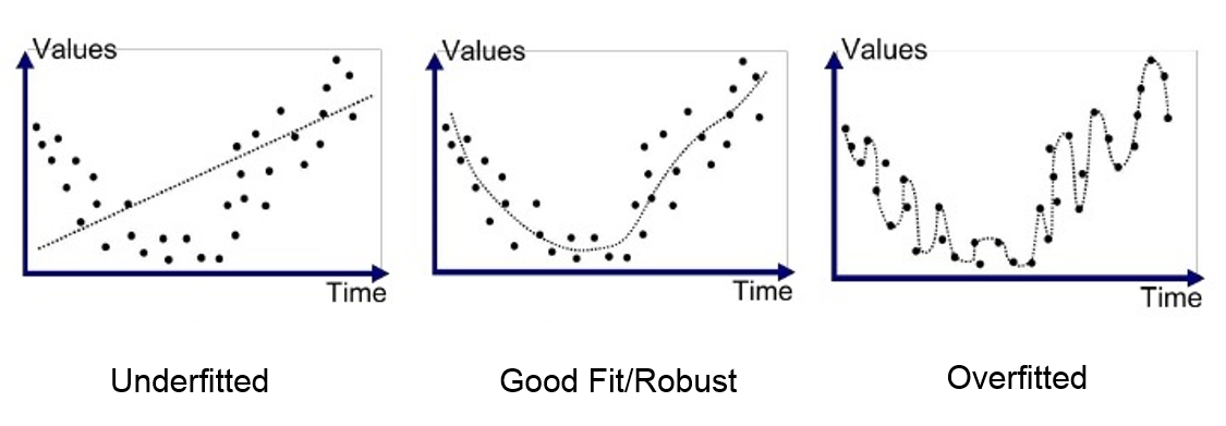
$$MSE_{train} = 0, \quad MSE_{test} \gg 0$$

Lagrange Interpolation

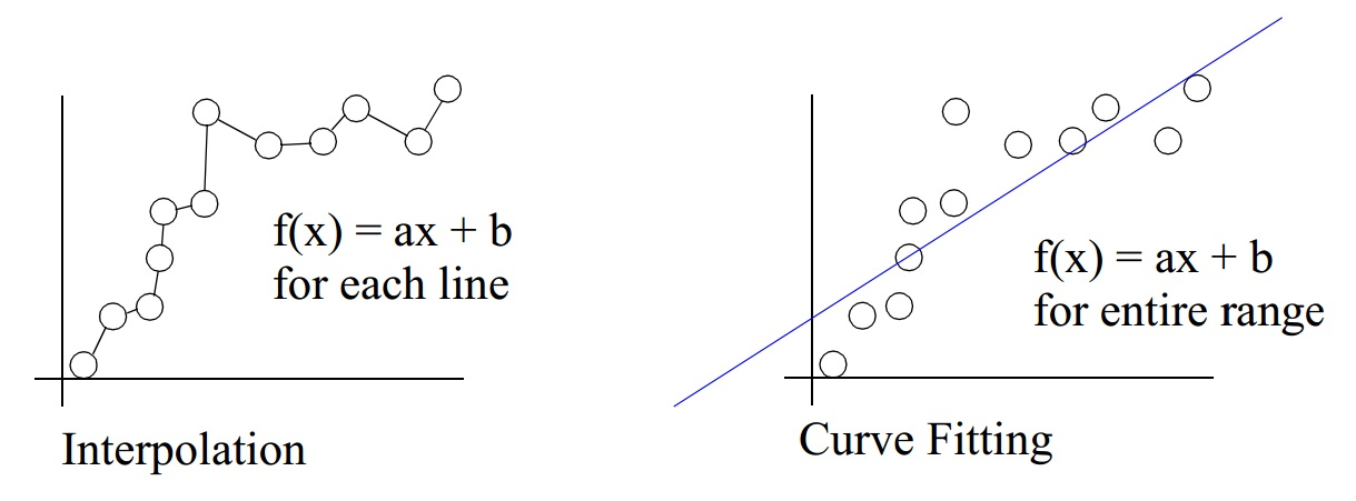
Theorem. Given a set of $k + 1$ distinct data points

$$(x_{0},y_{0}),\ldots ,(x_{j},y_{j}),\ldots ,(x_{k},y_{k})$$

The Lagrange interpolation is defined as

$$L(x):=\sum _{j=0}^{k}y_{j}\ell _{j}(x)$$

where Lagrange Polynomials for $0\leq j\leq k$ have the property:

$${\displaystyle \ell _{j}(x_{i})=\delta _{ji}={\begin{cases}1,&{\text{if }}j=i\\0,&{\text{if }}j\neq i\end{cases}},}$$

Lagrange Interpolation

It can be seen that the Lagrange Polynomials for $0\leq j\leq k$ can be defined as:

$$\begin{aligned} \ell _{j}(x)&:=\prod _{\begin{smallmatrix}0\leq m\leq k\\m\neq j\end{smallmatrix}}{\frac {x-x_{m}}{x_{j}-x_{m}}}\\&={\frac {(x-x_{0})}{(x_{j}-x_{0})}}\cdots {\frac {(x-x_{j-1})}{(x_{j}-x_{j-1})}}{\frac {(x-x_{j+1})}{(x_{j}-x_{j+1})}}\cdots {\frac {(x-x_{k})}{(x_{j}-x_{k})}}\end{aligned}$$

Generalized Lagrange Functions

The Lagrange Polynomials for $0\leq j\leq k$ can be defined as:

$$\ell^\phi _{j}(x):=\prod _{\begin{smallmatrix}0\leq m\leq k\\m\neq j\end{smallmatrix}}{\frac {\phi(x)-\phi(x_{m})}{\phi(x_{j})-\phi(x_{m})}}$$

where $\phi$ is an arbitrary smooth function and sufficiently differentiable.

Generalized Lagrange Functions

With different choices of $\phi(x)$, many new basis functions can be generated at different intervals:

Classic Polynomial                                                $\phi(x)=x$

Fractional Lagrange functions                            $\phi(x) = x^\delta$

Exponential Lagrange functions                        $\phi(x) = e^x$

Rational Lagrange functions                              $\phi(x) = \frac{x+L}{x-L}$

Fourier Lagrange functions                               $\phi(x) = sin(x)$