Alireza Afzal Aghaei
Graduate student at SBU
Suppose a man is at top of the valley and he wants to get to the bottom of the valley. So he goes down the slope.
He decides his next position based on his current position and stops when he gets to the bottom of the valley which was his goal.
Take repeated steps in the opposite direction of the gradient of the function at the current point.
Gradient descent is a first-order iterative optimization algorithm for finding a local minimum of a differentiable function.
It performs two steps iteratively:
Consider some continuously differentiable real-valued function \(f: \mathbb{R} \rightarrow \mathbb{R}\).
Using a Taylor expansion we obtain
$$f(x + \epsilon) = f(x) + \epsilon f'(x) + \mathcal{O}(\epsilon^2).$$
Pick a fixed step size \(\eta > 0\), and choose \(\epsilon = -\eta f'(x)\):
$$f(x - \eta f'(x)) = f(x) - \eta f'^2(x) + \mathcal{O}(\eta^2 f'^2(x)).$$
If \(f'(x) \neq 0\), with a small enough \(\eta\) we have:
$$f(x - \eta f'(x)) \lessapprox f(x).$$
This means that, if we use
$$x \leftarrow x - \eta f'(x)$$
to iterate \(x\), the value of function \(f\) might decline.
Repeat the iterations until
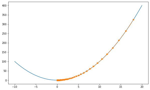
import numpy as np
def f(x):
return x**2
def df(x):
return 2 * x
a, b = -10, 20 # optimization domain
eta = 0.05 # learning rate
max_iterations = 53
x = 18 # x_initial
history = [x] # save function values
for epoch in range(max_iterations):
x = x - eta * df(x) # x = x - eta * df/dx
history.append(x)
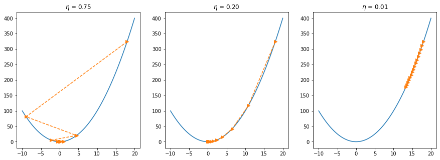
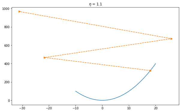
print('final x =', x)If we use an excessively high learning rate, \(\mathcal{O}(\eta^2 f'^2(x))\) might become significant. Hence we cannot guarantee that the iteration of \(x\) will be able to lower the value of \(f(x)\).
Suppose \(\mathbf{x} = [x_1, x_2, \ldots, x_d]^\top\) and objective function \(f: \mathbb{R}^d \to \mathbb{R}\). The gradient will be defined as:
$$\nabla f(\mathbf{x}) = \bigg[\frac{\partial f(\mathbf{x})}{\partial x_1}, \frac{\partial f(\mathbf{x})}{\partial x_2}, \ldots, \frac{\partial f(\mathbf{x})}{\partial x_d}\bigg]^\top.$$
Here the Taylor approximation takes the form
$$f(\mathbf{x} + \boldsymbol{\epsilon}) = f(\mathbf{x}) + \mathbf{\boldsymbol{\epsilon}}^\top \nabla f(\mathbf{x}) + \mathcal{O}(\|\boldsymbol{\epsilon}\|^2).$$
The corresponding gradient descent iteration:
$$\mathbf{x} \leftarrow \mathbf{x} - \eta \nabla f(\mathbf{x}).$$
Many of the machine learning models use gradient descent on their core:
Vanilla gradient descent, aka batch gradient descent, computes the gradient of the cost function w.r.t. to the parameters \(\theta\) for the entire training dataset
$$\theta = \theta - \eta \cdot \nabla_\theta J( \theta)$$
for i in range(n_epochs):
  params_grad = evaluate_gradient(loss_function, data, params)
params = params - learning_rate * params_gradStochastic gradient descent (SGD) in contrast performs a parameter update for each training example \(x^{(i)}\) and label \(y^{(i)}\):
$$\theta = \theta - \eta \cdot \nabla_\theta J( \theta; x^{(i)}; y^{(i)})$$
for i in range(nb_epochs):
  np.random.shuffle(data)
  for example in data:
    params_grad = evaluate_gradient(loss_function, example, params)
params = params - learning_rate * params_gradMini-batch gradient descent finally takes the best of both worlds and performs an update for every mini-batch of \(n\) training examples:
$$\theta = \theta - \eta \cdot \nabla_\theta J( \theta; x^{(i:i+n)}; y^{(i:i+n)})$$
for i in range(nb_epochs):
  np.random.shuffle(data)
  for batch in get_batches(data, batch_size=50):
    params_grad = evaluate_gradient(loss_function, batch, params)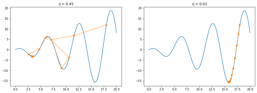
params = params - learning_rate * params_gradChoosing a proper learning rate can be difficult. A learning rate that is too small leads to painfully slow convergence, while a learning rate that is too large can hinder convergence and cause the loss function to fluctuate around the minimum or even to diverge.
Learning rate schedules try to adjust the learning rate during training by e.g. annealing, i.e. reducing the learning rate according to a pre-defined schedule or when the change in objective between epochs falls below a threshold. These schedules and thresholds, however, have to be defined in advance and are thus unable to adapt to a dataset's characteristics.
Additionally, the same learning rate applies to all parameter updates. If our data is sparse and our features have very different frequencies, we might not want to update all of them to the same extent, but perform a larger update for rarely occurring features.
By Alireza Afzal Aghaei


