


Alireza Afzal Aghaei
Graduate student at SBU
Alireza Afzal Aghaei
Maryam Babaei
An abbreviation of "matrix laboratory"
Invented by Cleve Moler in the 1970s
It is a proprietary numeric computing environment
Developed and supported by MathWorks
It's a multi-paradigm interpreted programming language
Its kernel is written in C/C++ programming languages
Matrix operations in MATLAB are built on LAPACK
MATLAB GUI is written in the Java programming language
GNU Octave
Free - Open Source
Based on Python
online version: octave-online.net, tutorialspoint, etc.
Mathematica, Maple
Proprietary
Computer Algebra System (CAS)
Julia
Free - Open Source
SageMath, Scilab, Maxima, etc.
In Matlab, the matrix is chosen as a basic data element
A scaler value is a \(1\times 1\) matrix
A vector is a \(1\times N\) or \(N\times 1\) matrix
A string is a vector of characters
Column-major layout for storing arrays
The elements of the columns are contiguous in memory
Numeric
int8, int16, int32, int64
uint8, uint16, uint32, uint64,
single, double
String
Cell-Array
Arrays that can contain data of varying types and sizes
Struct
Arrays with named fields that can contain data of varying types and sizes
>> x = 10; % data assignment for a scaler
>> x = [10]; % data assignment for a scaler

>> vec = [1 2 3]; % data assignment for a row vector
>> vec = [1, 2, 3]; % data for assignment for a row vector

>> vec = [1; 2; 3]; % data for assignment for a column vector

>> mat = [1, 2, 3; 4, 5, 6]; % data for assignment for a matrix

>> mat = [1 2 3; 4 5 6]; % data for assignment for a matrix

>> str = 'Hello world!'>> format long
>> pi
3.141592653589793
>> format short
>> pi
3.1416
>> format shortE
>> pi
3.1416e+00
>> format rat
>> pi
355/113 >> x = 10;
>> y = [pi -2 11];
>> disp(x)
10
>> fprintf('%d \n', x)
10
>> fprintf('%.2f \n', x)
10.00
>> disp(v)
3.1416 -2.0000 11.0000
>> fprintf('%.2f ', v)
3.14 -2.00 11.00
>> fprintf('%.2f # ', v)
3.14 # -2.00 # 11.00 # >> a = [1 2 3];
>> b = [2 5 8];
>> a + b
3 7 11
>> b - a
1 3 5
>> a * 9 % If the multiplier is a scalar
9 18 27
>> a + 1 % If the adder is a scalar
2 3 4>> a = [1 2; 3 4];
>> b = [1 5; 2 7];
>> a * b
5 19
11 43
>> a * a % matrix power
7 10
15 22
>> a ^ 2 % matrix power
7 10
15 22
>> a .^ 2 % elementwise power
1 4
9 16>> a = [1 2; 3 4];
>> b = [10, 20, 30];
>> c = [10; 20; 30];
>> a' % transpose of a
1 3
2 4
>> b'
10
20
30
>> c'
10 20 30>> a = [1 2 3];
>> b = [2 5 8];
>> a .* b % Hadamard product
2 10 24
>> dot(a, b) % inner product (dot product)
36
>> a * b' % inner product
36
>> a' * b % outer product
2 5 8
4 10 16
6 15 24>> v = [16 5 9 4 2 11 7 14];
>> v(3) % Extract the third element
9
>> v(3:7) % Extract the third through the seventh elements
9 4 2 11 7
>> v([1:3 5:8]) % Extract halves of v
16 5 9 2 11 7 14
>> v([5:8 1:3]) % Extract and swap the halves of v
2 11 7 14 16 5 9
>> v(end) % Extract the last element
14
>> v(5:end) % Extract the fifth through the last elements
2 11 7 14>> v = [16 5 9 4 2 11 7 14];
>> v(1:2:end) % Extract all the odd elements
16 9 2 7
>> v(end:-1:1) % Reverse the order of elements
14 7 11 2 4 9 5 16
>> v([2 3 4]) = [10 15 20] % Replace some elements of v
16 10 15 20 2 11 7 14
>> v([2 3]) = 30 % Replace second and third elements by 30
16 30 30 20 2 11 7 14
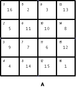
>> A = [16, 2, 3, 13;
	5, 11, 10, 8;
	9, 7,  6, 12;
	4, 14, 15, 1];

>> A(2,4)   % Extract the element in row 2, column 4
	8

>> A(2:4, 1:2)
    5          11
    9           7
    4          14

>> A(3, :)   % Extract third row
	9   7   6   12

>> A(:, end)   % Extract last column
    13
    8
    12
1>> A = [16, 2, 3, 13;
5, 11, 10, 8;
9, 7, 6, 12;
4, 14, 15, 1];
>> A([6 12 15])
11 15 12
>> B = [1 3; 7 5];
>> A(B)
16 9
7 2
>> A(:)' % reshape matrix to a column, then transpose it
16 5 9 4 2 11 7 14 3 10 6 15 13 8 12 1
Column-major layout
>> v = 1:5  %staring from 1 upto 5
    1  2  3  4  5

>> v = 1:2:11  %staring from 1 with an increment 2 and upto 11
    1  3  5  7  9  11

>> v = 6:-1:1
    6   5   4   3   2   1

>> v = -1:-1:-6
   -1  -2  -3  -4  -5  -6

>> v = -1:-2:-10
-1 -3 -5 -7 -9>> A = ones(3, 2)
1 1
1 1
1 1
>> A = zeros(1, 5)
0 0 0 0 0
>> A = eye(3)
1 0 0
0 1 0
0 0 1
>> A = magic(3)
8 1 6
3 5 7
4 9 2>> rng(n) % sets the random seed to n
>> r = rand % returns a single uniformly distributed random number in the interval (0,1).
>> r = rand(n) % returns an n-by-n matrix of random numbers.
>> X = randn % returns a random scalar drawn from the standard normal distribution.
>> X = randn(n) % returns an n-by-n matrix of normally distributed random numbers.
>> X = randi(imax) % returns a pseudorandom scalar integer between 1 and imax.
>> X = randi(imax, n) %returns an n-by-n matrix of pseudorandom integers drawn from the discrete uniform distribution on the interval [1, imax].>> r = rand(3)
0.8147 0.0975 0.1576
0.9058 0.2785 0.9706
0.1270 0.5469 0.9572
>> r = randn(3)
0.5377 -1.3077 -1.3499
1.8339 -0.4336 3.0349
-2.2588 0.3426 0.7254
>> r = randi(10, 5)
9 1 2 2 7
10 3 10 5 1
2 6 10 10 9
10 10 5 8 10
7 10 9 10 7>> A = [1 3; 6 9; 6 11];
>> B = [3 3 5; 9 9 7; 11 4 -1];
>> size(A)
3 2
>> size(B)
3 3
>> size(A, 1)
3
>> size(A, 2)
2
>> numel(A)
6
>> numel(B)
9>> A = [1 3; 6 9; 6 11];
>> B = [3 3; 9 9; 4 -1];
>> C = cat(2, A, B)
1 3 3 3
6 9 9 9
6 11 4 -1
>> D = cat(1, A, B)
1 3
6 9
6 11
3 3
9 9
4 -1
>> reshape(C, 2, 6)
1 6 9 3 4 9
6 3 11 9 3 -1>> A = [1 4 -3 2];
>> B = [1 4 -11; 7 -3 2];
>> sum(A) % sum of all elements
4
>> sum(B) % sum of each column
8 1 -9
>> sum(sum(B))
0
>> sum(B(:))
0
>> mean(A) % average of all elements
1
>> mean(B) % average of each column
4.0000 0.5000 -4.5000>> A = [1 0 -3 2 0 4 3.3 5.7];
>> round(A) % rounds the elements to nearest integer
1 0 -3 2 0 4 3 6
>> sort(A, 'ascend') % for sorting, 'ascend' or 'descend'
-3.000 0 0 1.000 2.000 3.300 4.000 5.700
>> find(A) % returns the linear indices corresponding to non-zero entries of the array
1 3 4 6 7 8
>> v = [2, 8, -3];

>> p = poly2sym(v)
       2
    2⋅x  + 8⋅x - 3

>> subs(p, 3)
	39

>> polyval(v, 3)
	39

>> roots(v)
  -4.3452
0.3452>> x = sym('x'); % or for simplicity "syms x"
>> y = sym('y','real');
>> z = sym('z','positive');
>> t = sym('t',{'positive','integer'});
>> x ^ 2 + 3 * x
2
x + 3⋅x
>> a = sym('a',[1 4])
[a1, a2, a3, a4]
>> sqrt(sym(1234567))
√1234567
>> exp(sym(pi))
π
ℯ >> syms x
>>> y = sin(x + 1) + x ^ 2;
>> subs(y, x, 1)
sin(2) + 1
>> diff(y,x) % differentiate symbolic expression
2⋅x + cos(x + 1)
>> int(y) % integrate symbolic expression
3
x
── - cos(x + 1)
3
>> z = int(y, x, 0, 2) % definite integral
cos(1) - cos(3) + 8/3
>> double(z)
4.1970x = 1
A = rand(2, 3)
% etc.The Matlab scripts are stored in .m files:
The scripts usually start with these commands
clear % clear workspace variables
close % close all figure windows
clc % clear screenfunction [y, z] = my_func(x1, x2)
y = sin(x1);
z = cos(x2);
endSave the function in a .m file, named my_func.
Now, in the same directory, call the function:
>> my_func(1, 2)
	0.8415

>> [a, b] = my_func(1, 2)
0.8415 -0.4161>> f = @my_func % function handle
>> f(1, 2)
0.8415
>> [a, b] = f(1, 2)
0.8415 -0.4161>> f = @(x) sin(x) + sqrt(x); % anonymous function
>> f(1)
1.8415
>> quad(f, 0, 2) % numerical integration
3.3018
>> syms x;
>> double(int(f(x), x, 0, 2));
3.3018
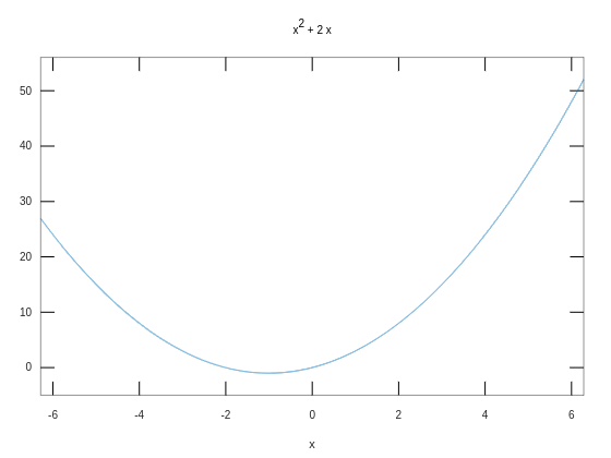
>> syms x;

>> y = x ^ 2 + 2 * x;
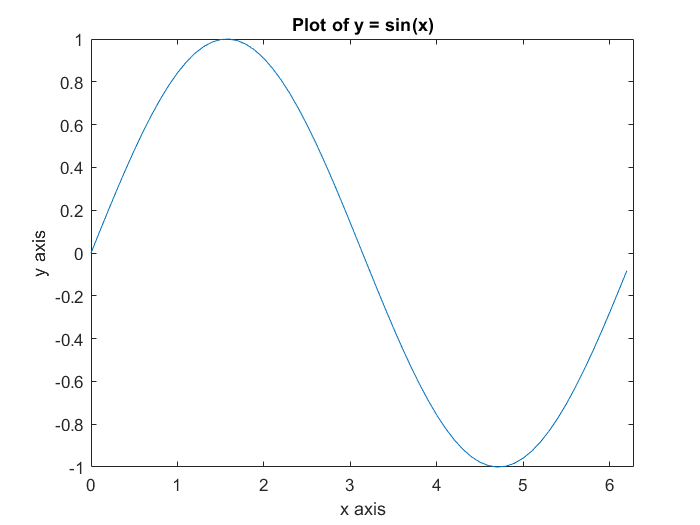
>> ezplot(y)x = 0: .1 : 2 * pi; % Creates a vector that starts at 0 and ends at 2*pi with increments of .1
y = sin(x);
plot(x,y)
xlabel('x axis')
ylabel('y axis')
title('Plot of y = sin(x)')
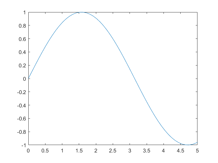
axis([0 2*pi -1 1]) x = linspace(0, 10);
y = sin(x);
plot(x,y)
xlim([0 5]) % sets the x-axis limits for the current axes or chart. Specify limits as a two-element vector of the form [xmin xmax], where xmax is greater than xmin.[X, Y] = meshgrid(1:0.5:10,1:20);
Z = sin(X) + cos(Y);
surf(X,Y,Z) %creates a three-dimensional surface plot, which is a three-dimensional surface that has solid edge colors and solid face colors. The function plots the values in matrix Z as heights above a grid in the x-y plane defined by X and Y. The color of the surface varies according to the heights specified by Z.1 > 5 % ans = 0
10 >= 10 % ans = 1
3 ~= 4 % Not equal to -> ans = 1
3 == 3 % equal to -> ans = 1
3 > 1 && 4 > 1 % AND -> ans = 1
3 > 1 || 4 > 1 % OR -> ans = 1
~1 % NOT -> ans = 0
>> A = magic(5);
   17   24    1    8   15
   23    5    7   14   16
    4    6   13   20   22
   10   12   19   21    3
   11   18   25    2    9

>> B = A > 18
  0  1  0  0  0
  1  0  0  0  0
  0  0  0  1  1
  0  0  1  1  0
  0  0  1  0  0

>> C = A(B)
   23
   24
   19
   25
   20
   21
22a = input('Enter the value: ')
if (a > 23)
disp('Greater than 23')
elseif (a == 23)
disp('a is 23')
else
disp('neither condition met')
endn = input('Enter a number: ');
switch n
case -1
disp('negative one')
case 0
disp('zero')
case 1
disp('positive one')
otherwise
disp('other value')
end% for loop
for k = 1:5
disp(k)
end
% while loop
k = 0;
while (k < 5)
k = k + 1;
end% Execute statements and catch resulting errors
a = ones(4);
b = zeros(3);
try
c = [a; b];
catch ME
disp(ME)
end
% MException with properties:
% identifier: 'MATLAB:catenate:dimensionMismatch'
% message: 'Dimensions of arrays being concatenated are not consistent.'
% cause: {0×1 cell}
% stack: [0×1 struct]%% cell arrays
>> syms x
>> a = {'one', zeros(3), sin(x)};
>> a(1)
'one'
%% structures
>> A.b = {'one','two'};
>> A.c = [1 2];
>> A.d.e = false;
>> A.c
[1 2]classdef WaypointClass % The class name.
properties % The properties of the class behave like Structures
latitude
longitude
end
methods
% This method that has the same name of the class is the constructor.
function obj = WaypointClass(lat, lon)
obj.latitude = lat;
obj.longitude = lon;
end
% Other functions that use the Waypoint object
function r = multiplyLatBy(obj, n)
r = n*[obj.latitude];
end
% If we want to add two Waypoint objects together without calling
% a special function we can overload Matlab's arithmetic like so:
function r = plus(o1,o2)
r = WaypointClass([o1.latitude] +[o2.latitude], ...
[o1.longitude]+[o2.longitude]);
end
end
end% We can create an object of the class using the constructor
a = WaypointClass(45.0, 45.0)
% Class properties behave exactly like Matlab Structures.
a.latitude = 70.0
a.longitude = 25.0
% Methods can be called in the same way as functions
ans = multiplyLatBy(a,3)
% The method can also be called using dot notation. In this case, the object
% does not need to be passed to the method.
ans = a.multiplyLatBy(1/3)
% Matlab functions can be overloaded to handle objects.
% In the method above, we have overloaded how Matlab handles
% the addition of two Waypoint objects.
b = WaypointClass(15.0, 32.0)
c = a + b>> v = [1 -2 3];
>> norm(v,1)
6
>> norm(v,2)
3.7417
>> norm(v,'inf')
3
>> X = [2 0 1;
-1 1 0;
-3 3 0];
>> norm(X,1)
6
>> norm(X,2)
4.7234
>> norm(X,'inf')
6
>> norm(X,'fro')
5>> cond(magic(3))
4.3301
>> cond(magic(11))
11.102
>> cond(ones(11))
Inf
>> cond(eye(11))
1
>> hilb(sym(4))
⎡ 1 1/2 1/3 1/4⎤
⎢ ⎥
⎢1/2 1/3 1/4 1/5⎥
⎢ ⎥
⎢1/3 1/4 1/5 1/6⎥
⎢ ⎥
⎣1/4 1/5 1/6 1/7⎦
>> cond(hilb(4))
1.5514e+04
>> cond(hilb(5))
4.7661e+05
>> cond(hilb(6))
1.4951e+07>> A = [1 1;
1 1];
>> B = [-1 1;
1 -1];
>> null(A)'
0.7071 -0.7071
>> null(A, 'r')'
-1 1
>> null(B)
0.7071 0.7071
>> null(B, 'r')'
1 1>> A = [4 11 14;
8 7 -2];
>> size(A)
2 3
>> issymmetric(A)
0
>> A * A'
333 81
81 117
>> size(A * A')
2 2
>> issymmetric(A * A')
1
>> A' * A
80 100 40
100 170 140
40 140 200
>> size(A' * A)
3 3
>> issymmetric(A' * A)
1>> B = [3 2 15;
4 7 11;
5 6 -3];
>> issymmetric(B)
0
>> B' * B
50 64 74
64 89 89
74 89 355
>> issymmetric(B' * B)
1
>> B * B'
238 191 -18
191 186 29
-18 29 70
>> issymmetric(B * B')
1
>> B + B'
6 6 20
6 14 17
20 17 -6
>> issymmetric(B + B')
1>> A = [1 -2 4;
-5 2 0;
1 0 3]
>> d = det(A) % returns the determinant of square matrix A.
-32
>> B = rand(2,3);
>> det(B)
% error: det: A must be a square matrix>> A = [1 2 3;
2 4 6;
7 -1 11]
>> B = [-4 3 2;
1 11 9;
2 4 7]
>> rank(A)
2
>> det(A)
0
>> rank(B)
3
>> det(B)
-167The rank of a matrix A is the dimension of the vector space spanned by its columns.
>> A = [1 2 1;
       -1 -2 5;
        3 1 -1]

>> M11 = det(A(2:end, 2:end))
	-3

>> M23 = det(A([1,3], [1, 2]))
	-5

>> % Chat = [M11, M12, M13; M21, M22, M23; M31, M32, M33];

>> % C = -1 ^ (i+j) Chat(i, j)

>> adjoint(A); % C'
   -3.0000    3.0000   12.0000
   14.0000   -4.0000   -6.0000
5.0000 5.0000 0.0000>> A = [1 2 1;
-1 -2 5;
3 1 -1]
>> det(A)
30
>> adjoint(A);
-3.0000 3.0000 12.0000
14.0000 -4.0000 -6.0000
5.0000 5.0000 0.0000
>> B = inv(A)
-0.1000 0.1000 0.4000
0.4667 -0.1333 -0.2000
0.1667 0.1667 0
>> B * A % or A * B
1.0000 0 -0.0000
0.0000 1.0000 0.0000
0 0 1.0000A generalization of the inverse matrix
If the columns of a matrix \(A\) are linearly independent
\(A^T A\) is invertible:
$$A^\dagger = (A^T A)^{-1} A^T$$
\(A^\dagger\) is a left inverse of \(A\) , what means: \(A^\dagger A = I\) .
If the rows of the matrix are linearly independent: $$A^\dagger = A^T (A A^T)^{ -1}$$
This is a right inverse of \(A\) , what means: \(A A^\dagger = I\)
>> A = randn(3,2)
   0.3649   1.6099
   0.4730  -1.2022
   0.6131   0.3984

>> B = pinv(A)

  0.368501   0.765524   0.821077
  0.360588  -0.334517   0.043466

>> C = inv(A' * A) * A'
   0.368517   0.765591   0.821079
   0.360589  -0.334527   0.043472

>> B * A
   1.0000e+00  -5.3536e-17
7.3552e-17 1.0000e+00syms lambda;
A = [80, 100, 40;
100, 170, 140;
40, 140, 200];
N = size(A); % 3 3
char_poly = det( A - lambda * eye(N));
% 31200⋅λ + (80 - λ)⋅(170 - λ)⋅(200 - λ) - 2720000
expand(char_poly)
% 3 2
% - λ + 450⋅λ - 32400⋅λ
coeffs = sym2poly(char_poly);
% -1 450 -32400 0
eig_vals = roots(coeffs);
% 360 90 0syms lambda;
A =[-0.365671 0.220302 0.030732;
-1.632830 1.207995 2.139820;
0.044537 0.616437 0.158060]
N = size(A); % 3 3
char_poly = det( A - lambda * eye(N));
coeffs = sym2poly(char_poly);
% -1.0000 1.0004 1.2693 0.4578
eig_vals = roots(coeffs);
% 1.8305 + 0i
% -0.4150 + 0.2790i
% -0.4150 - 0.2790isyms lambda;
A = [80, 100, 40;
100, 170, 140;
40, 140, 200];
N = size(A);
char_poly = det( A - lambda * eye(N));
coeffs = sym2poly(char_poly);
eig_vals = roots(coeffs);
% 0 360 90
eig_vecs = zeros(N, N);
for i=1:size(eig_vals,1)
B = A - eig_vals(i) * eye(N);
eig_vec = null(B);
eig_vecs(:,i) = eig_vec;
end
%{
0.6667 -0.3333 0.6667
-0.6667 -0.6667 0.3333
0.3333 -0.6667 -0.6667
%}>> e = eig(A) % returns a column vector containing the eigenvalues of square matrix A.
>> [V, D] = eig(A) % returns diagonal matrix D of eigenvalues and matrix V whose columns are the corresponding right eigenvectors, so that A*V = V*D.
>> [V, D, W] = eig(A) % also returns full matrix W whose columns are the corresponding left eigenvectors, so that W'*A = D*W'.
>> e = eig(A, B) % eturns a column vector containing the generalized eigenvalues of square matrices A and B.>> A = [80, 100, 40;
100, 170, 140;
40, 140, 200];
>> [v, d] = eig(A);
%{
v =
0.6667 0.6667 0.3333
-0.6667 0.3333 0.6667
0.3333 -0.6667 0.6667
d =
-2.3143e-14 0 0
0 9.0000e+01 0
0 0 3.6000e+02
%}>> B = [-0.365671 0.220302 0.030732;
-1.632830 1.207995 2.139820;
0.044537 0.616437 0.158060];
>> [v, d] = eig(B);
%{
v =
0.0984 + 0i 0.1030 + 0.4305i 0.1030 - 0.4305i
0.9329 + 0i -0.6478 + 0i -0.6478 - 0i
0.3465 + 0i 0.5700 + 0.2440i 0.5700 - 0.2440i
d =
1.8305 + 0i 0 0
0 -0.4150 + 0.2790i 0
0 0 -0.4150 - 0.2790i
%}>> A = [1 7 3; 2 9 12; 5 22 7];
>> e = eig(A);
25.5548
-0.5789
-7.9759
>> [V, D, W] = eig(A)
V =
-0.2610 -0.9734 0.1891
-0.5870 0.2281 -0.5816
-0.7663 -0.0198 0.7912
D =
25.5548 0 0
0 -0.5789 0
0 0 -7.9759
W =
-0.1791 -0.9587 -0.1881
-0.8127 0.0649 -0.7477
-0.5545 0.2768 0.6368>> d = eigs(A) % returns a vector of the six largest magnitude eigenvalues of matrix A.
>> d = eigs(A, k) %returns the k largest magnitude eigenvalues.
>> [V, D] = eigs(___) % returns diagonal matrix D containing the eigenvalues on the main diagonal, and matrix V whose columns are the corresponding eigenvectors.
>> [V, D, flag] = eigs(___) %also returns a convergence flag. If flag is 0, then all the eigenvalues converged.>> A = rand(3, 3);
>> e = eig(A);
>> [trace(A), sum(e)]
1.9038 1.9038
>> [det(A), prod(e)]
-0.1270 -0.1270
Every square matrix over a commutative ring (such as the real or complex field) satisfies its own characteristic equation.
>> syms lambda;
>> A = [7, 10, 7; 7, 1, 6; 3, 4, 7]
>> N = size(A);
>> char_poly = det( A - lambda * eye(N));
               3       2
            - λ  + 15⋅λ  + 52⋅λ - 254

>> - A ^ 3 + 15 * A ^ 2 + 52 * A - 254 * eye(N)
    0   0   0
    0   0   0
    0   0   0

>> coeffs = sym2poly(char_poly);
>> polyvalm(coeffs, A);
    0   0   0
    0   0   0
0 0 0An \(n \times n\) symmetric real matrix \(M\) is said to be positive-definite if \(x^T M x > 0\) for all non-zero \(x\) in \(\mathbb{R}^n\).
>> A = [1 -1 0; -1 5 0; 0 0 7];
>> B = [1 -1 0; -1 5 0; 0 0 -1];

try
    chol(A)
    disp('Matrix is symmetric positive definite.')
catch ME
    disp('Matrix is not symmetric positive definite')
end

%    1.0000  -1.0000        0
%         0   2.0000        0
%         0        0   2.6458
% Matrix is symmetric positive definite.


try
    chol(B)
    disp('Matrix is symmetric positive definite.')
catch ME
    disp('Matrix is not symmetric positive definite')
end

% Matrix is not symmetric positive definite>> A = [1 -1 0; -1 5 0; 0 0 7];
>> B = [1 -1 0; -1 5 0; 0 0 -1];
e = eig(A);
isposdef = all(e > 0);
if isposdef
disp('Matrix is symmetric positive definite.')
else
disp('Matrix is not symmetric positive definite')
end
% Matrix is symmetric positive definite.
e = eig(B);
isposdef = all(e > 0);
if isposdef
disp('Matrix is symmetric positive definite.')
else
disp('Matrix is not symmetric positive definite')
end
% Matrix is not symmetric positive definiteThe Frobenius companion matrix of the monic polynomial
$$p(t)=c_{0}+c_{1}t+\cdots +c_{{n-1}}t^{{n-1}}+t^{n}$$ is the square matrix defined as
$$C(p)={\begin{bmatrix}0&1&0&\cdots &0\\0&0&1&\cdots &0\\\vdots &\vdots &\vdots &\ddots &\vdots \\0&0&0&\cdots &1\\-c_{0}&-c_{1}&-c_{2}&\cdots &-c_{{n-1}}\end{bmatrix}}$$
>> u = [1 0 -7 6];

>> A = compan(u);
     0     7    -6
     1     0     0
     0     1     0

>> eig(A)
   -3.0000
    2.0000
    1.0000
$$\begin{array}{ll}p(x) &= (x−1)(x−2)(x+3) \\ &=x^3 −7x+6\end{array}$$
>> S = [4, 11, 14;
        8, 7, -2];

>> A = S' * S
    80   100    40
   100   170   140
    40   140   200

>> [v, e] = eig(A);

>> sigma = sqrt(e)
         0 +  0.0000i
    9.4868 +       0i
   18.9737 +       0i

>>  V = v
     0.6667   0.6667   0.3333
    -0.6667   0.3333   0.6667
0.3333 -0.6667 0.6667>> S = [4, 11, 14;
8, 7, -2];
>> [u, sigma, v] = svd(S)
%{
u =
-0.9487 -0.3162
-0.3162 0.9487
sigma =
18.9737 0 0
0 9.4868 0
v =
-0.3333 0.6667 -0.6667
-0.6667 0.3333 0.6667
-0.6667 -0.6667 -0.3333
%}>> S = [4, 11, 14;
8, 7, -2];
>> [u, sigma, v] = svd(S)
>> u' * u
1.0000e+00 -9.3142e-17
-9.3142e-17 1.0000e+00
>> v' * v
1.0000e+00 3.0840e-16 -2.6214e-16
3.0840e-16 1.0000e+00 3.1148e-16
-2.6214e-16 3.1148e-16 1.0000e+00>> S = [4, 11, 14;
8, 7, -2];
>> [u, sigma, v] = svd(S)
for i=1:size(S, 1)
normSVi = norm(S * v(:, i));
fprintf('%.6f \t %.6f \n', normSVi, sigma(i,i))
end
%{
|| S v_i || sigma_i
18.973666 18.973666
9.486833 9.486833
%}>> s = svds(A) % returns a vector of the six largest singular values of matrix A.
>> s = svds(A, k) % returns the k largest singular values.
>> s = svds(A, k, sigma) % returns k singular values based on the value of sigma.
>> [U, S, V] = svds(___) % returns the left singular vectors U, diagonal matrix S of singular values, and right singular vectors V.
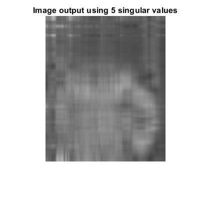
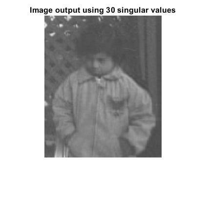
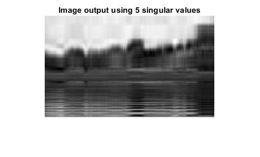
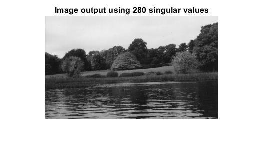
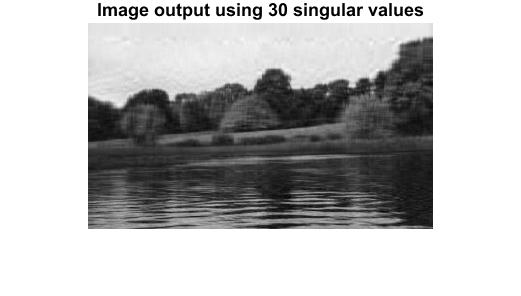
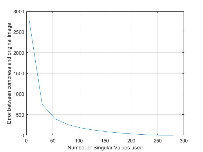
>> [U, S, V, flag] = svds(___) % also returns a convergence flag. If flag is 0, then all the singular values converged.% reading and converting the image
inImage = imread('pout.tif');
inImage = rgb2gray(inImage);
% since image data type is uint8
inImageD = double(inImage);
% decomposing the image using singular value decomposition
[U, S, V] = svd(inImageD);
% Using largest singular values to reconstruct the image
N = 10;
% Construct the Image using the selected singular values
D = U(:,1:N) * S(1:N, 1:N) * V(:, 1:N)';
ImageNew = uint8(D);
imshow(inImage)
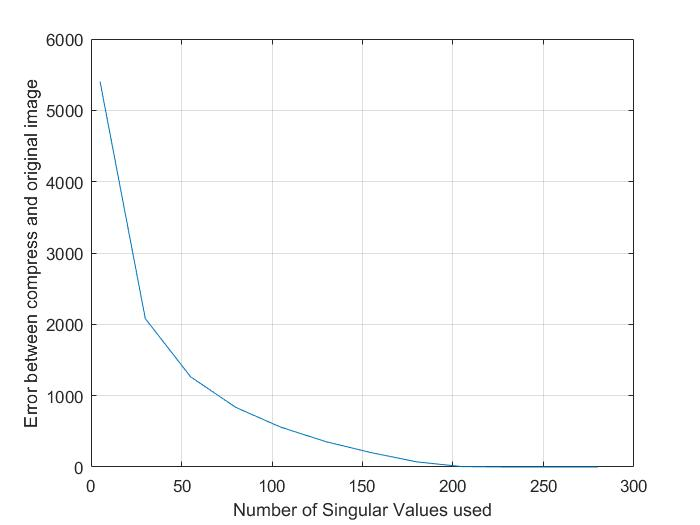
imshow(ImageNew)$$\text{Error =}\| img_{new} - img_{real} \|_F$$
autumn.tif
pout.tif
In the case of full rank square matrix \(A\), the system has a unique solution given by $$x =A^{-1}b$$
In the case of general rectangular matrix \(A\) we have: $$x = A^{\dagger}b$$ where \(A^{\dagger}\) is pseudo inverse of \(A\)
The numerical methods can also be employed to these systems
Direct methods
LU, Cholesky, QR
Iterative methods
Gauss seidel, Jacobi, Conjugate Gradient, GMRES
>>> A = [1 2 -3;
        -3 -1 1;
         1 -1 1]

>> b = [5; -8; 0];

>> x = inv(A) * b

   2.0000
   3.0000
   1.0000

>> x = A \ b % more efficient than inv(A) * b

   2.0000
   3.0000
1.0000By Alireza Afzal Aghaei


