Joint inference of mass-maps and cosmology with diffusion models


Benjamin Remy
Advancing Field-level and Simulation-based Inference for Cosmology,
Perimeter Institute for Theoretical Physics, June 2026
with Chihway Chang and Rebecca Willett
Weak lensing for cosmology
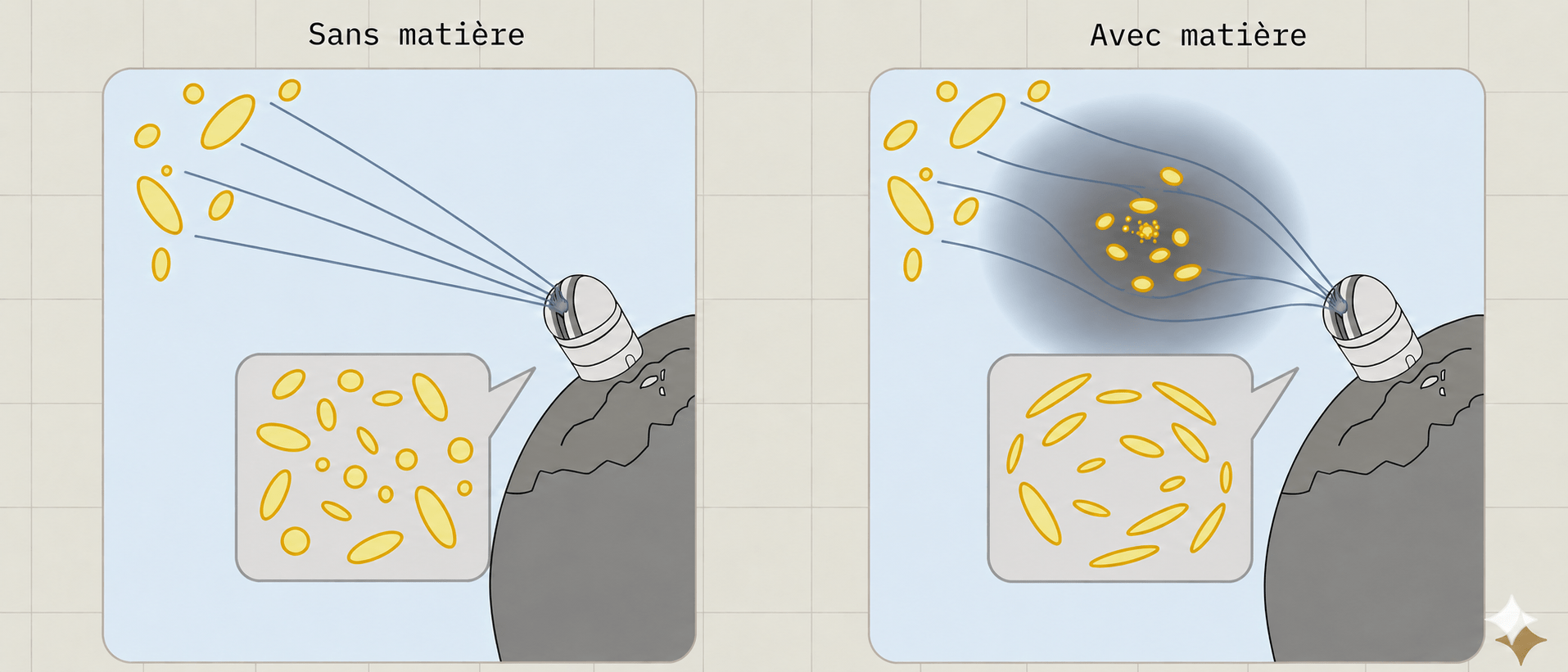
Credit: Jessie Muir adapted by Justine Zeghal
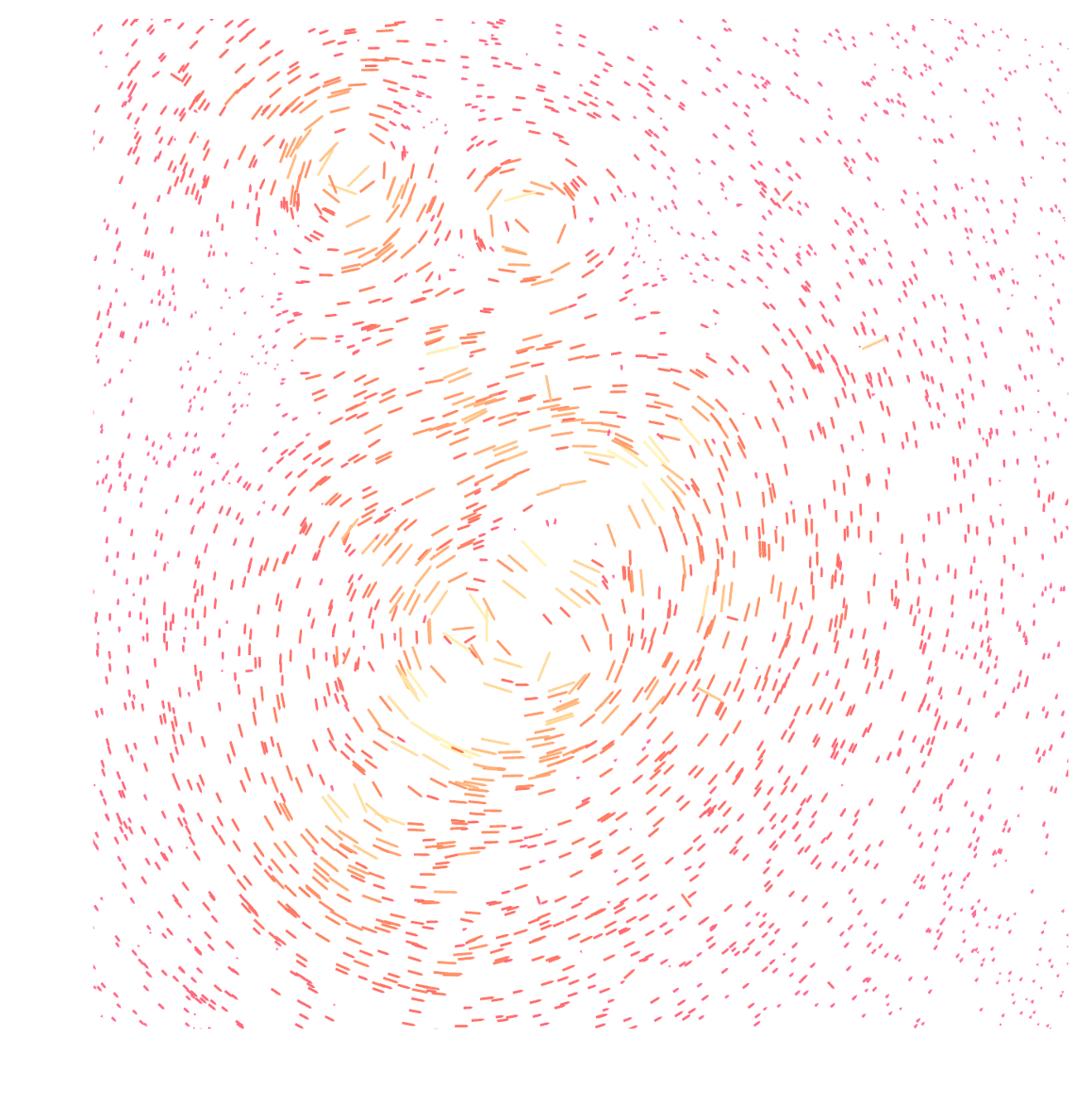
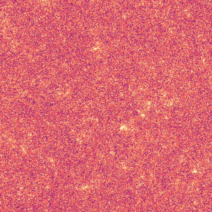
Shear
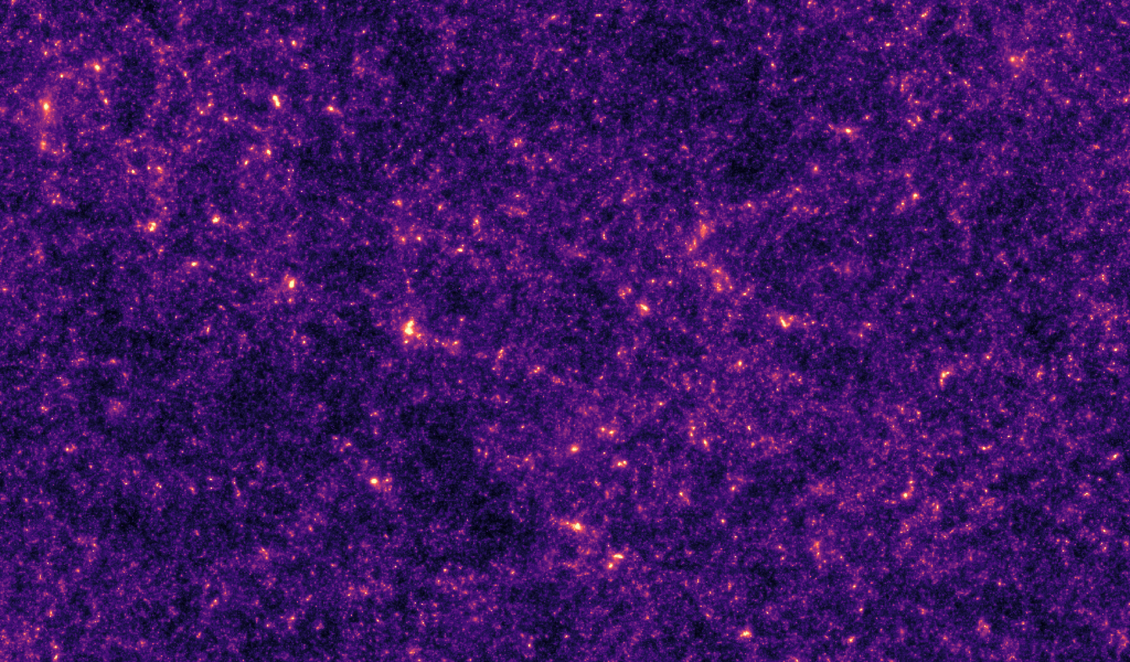
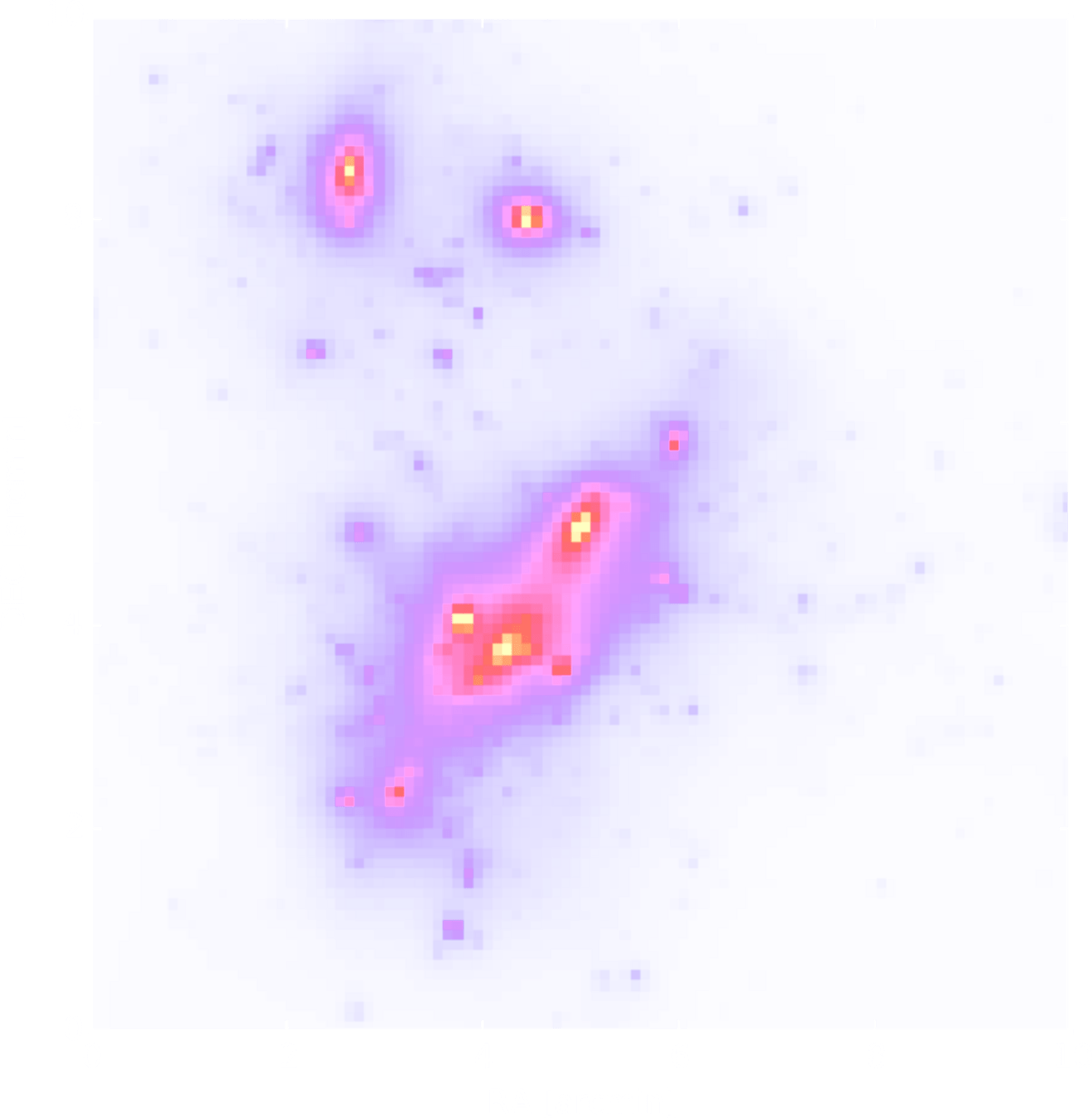
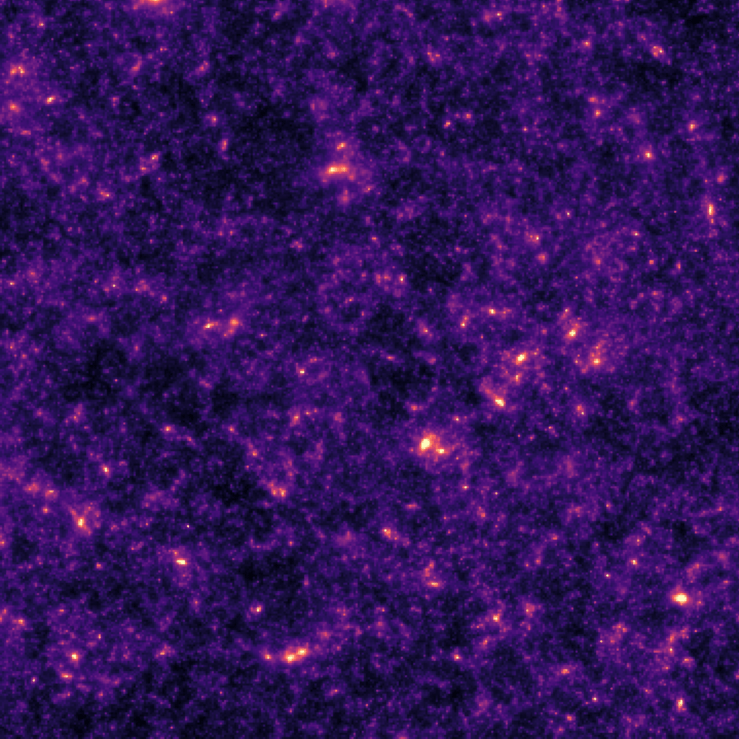
Convergence
\gamma
\kappa
How to optimally infer cosmology from observing ?
\gamma_\text{obs}
How to reconstruct with a non-linear model?
\kappa
\theta
Weak lensing mass-mapping as an inverse problem
\theta
N-body +
ray-tracing
(e.g. TNG, Gower Street)
\kappa
\kappa
\gamma^\text{obs}
p(\theta)
p(\kappa\mid \theta)
p(\gamma^{\text{obs}} \mid \kappa, \theta)
Forward model
\delta_\text{IC}
Inference (inverse problem)
p(\theta\mid \kappa, \gamma_\text{obs})
p(\kappa\mid \gamma_\text{obs})
\gamma^{\text{obs}}
Running N-body simulations, we
implicitly sample from the joint distribution
\theta, \kappa, \gamma \sim p(\theta)p(\kappa\mid \theta)p(\gamma\mid \kappa, \theta)
Likelihood-free inference uses simulations to learn
the implicit distributions
(posterior, likelihood, likelihood ratio)
(\theta, \kappa, \gamma)
Full field inference
Full field inference x Likelihood-free inference (LFI)
Field reconstruction
Cosmological inference
Targets
p(\theta \mid \gamma_\text{obs})
Targets
p(\kappa \mid \gamma_\text{obs}, \theta_\text{fid})
Posterior sampling with diffusion models (Remy et al. 2023)
LFI for weak lensing full field
LFI for weak lensing full field
How can we combine them in a joint inference framework ?
p(\theta, \kappa \mid \gamma_\text{obs})
Text
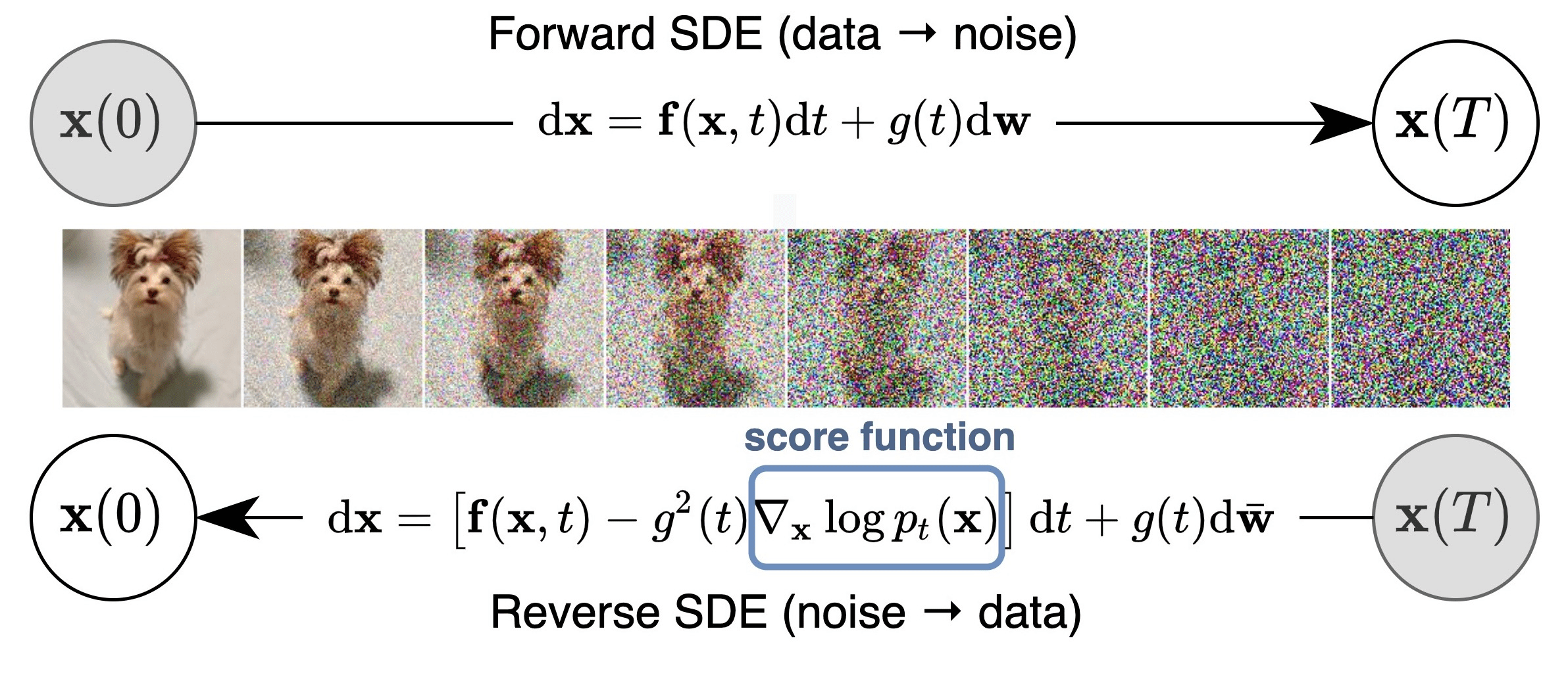
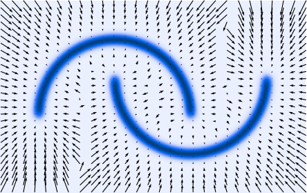
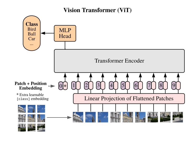
A diffusion model learns to reverse the noising process, by learning
the prior score function
\nabla_x \log p_t(x)
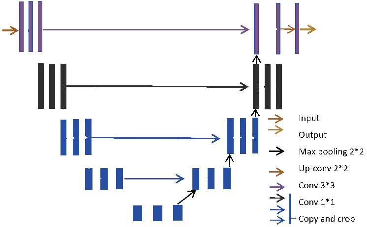
U-net architecture, well suited for 2D, 3D fields
But not for inferring cosmological parameters...
Tweedy formula
\color{blue}{d_\phi(x^\prime, t)}\color{black}{, \quad x^\prime=x+n, \quad n\sim\mathcal{N}(0,\sigma_t)}
\color{blue}{d_\phi(x^\prime, t) = x^\prime + \sigma_t^2 \nabla_x \log p_t(x)}
Posterior inference with diffusion model
A diffusion model learns to reverse the noising process, by learning
the posterior score function
\nabla_x \log p_t(x\mid y)
U-net architecture, well suited for 2D, 3D fields
But not for inferring cosmological parameters...
Tweedy formula
\color{blue}{d_\phi(x^\prime, t, y)}\color{black}{, \quad x^\prime=x+n, \quad n\sim\mathcal{N}(0,\sigma_t)}
\color{blue}{d_\phi(x^\prime, t, y) = x^\prime + \sigma_t^2 \nabla_x \log p_t(x \mid y)}
Posterior inference with diffusion model
p(\theta, \kappa)
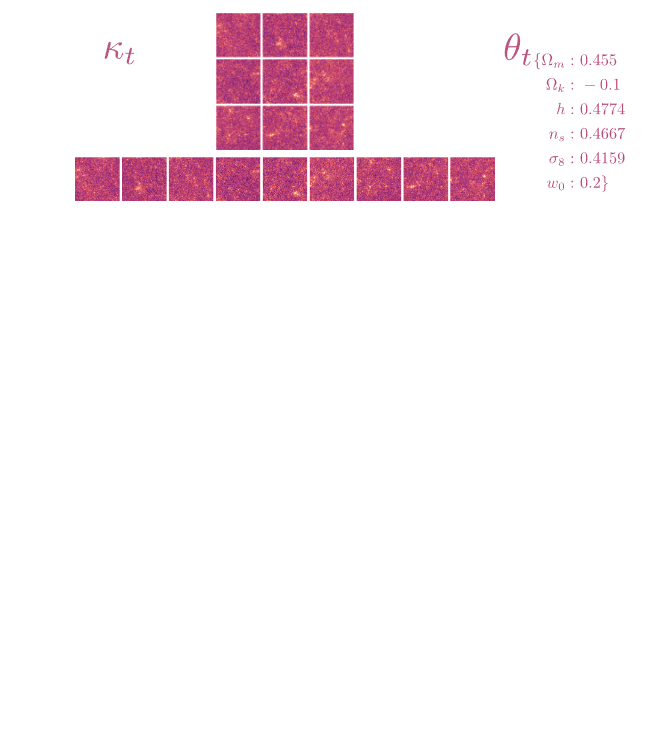
We need to model to design a denoiser architecture
to learn the score function.
\left[\theta_t, \kappa_t\right] = \left[\theta, \kappa\right] + \sigma_tn
d^\star(\theta_t, \kappa_t, \sigma_t) = \left[\theta^\star, \kappa^\star\right]
We learn the joint denoiser
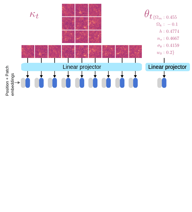
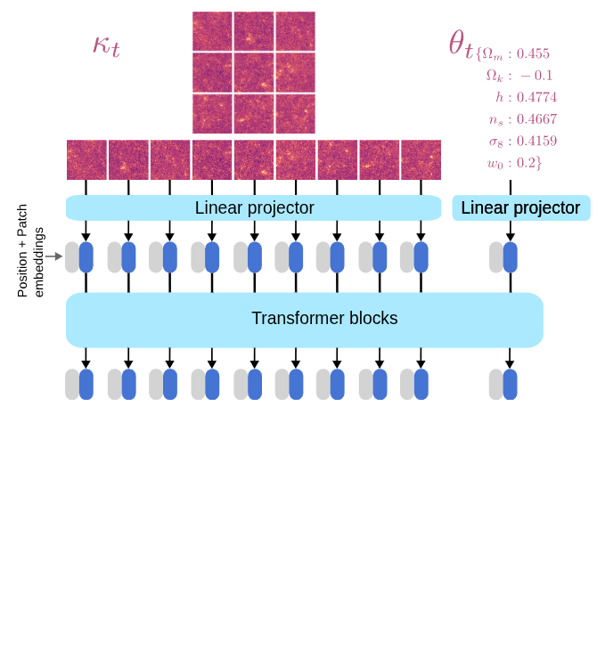
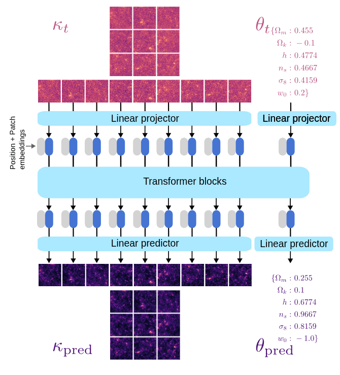
Learning the joint distribution
And now have the joint score function to run a diffusion model
\nabla_{\kappa_t, \theta_t} \log p(\kappa_t, \theta_t)
p(\kappa, \theta)
\nabla_{\kappa_t, \theta_t} \log p(\kappa_t, \theta \mid \gamma_{t}^\text{obs})
p(\kappa, \theta\mid \gamma_\text{obs})
Learning the joint distribution
We need to model to design a denoiser architecture
to learn the score function.
\left[\theta_t, \kappa_t\right] = \left[\theta, \kappa\right] + \sigma_tn
We learn the joint denoiser
And now have the joint score function to run a diffusion model
d^\star(\theta_t, \kappa_t, \sigma_t, \gamma_\text{obs}) = \left[\theta^\star, \kappa^\star\right] \mid \gamma_\text{obs}
Learning the joint distribution
p(\theta, \kappa)

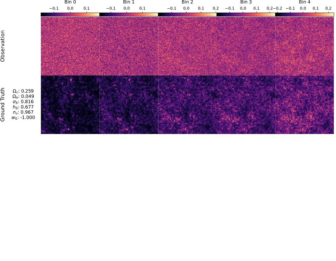
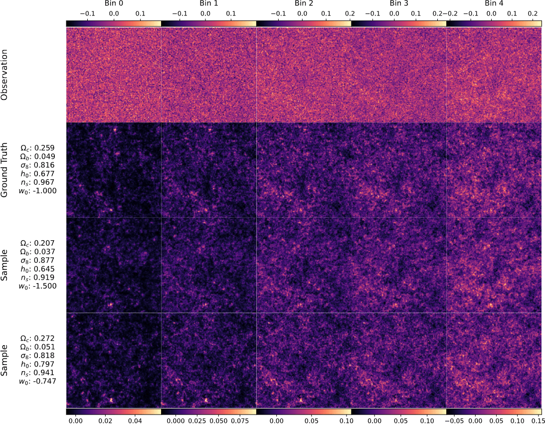
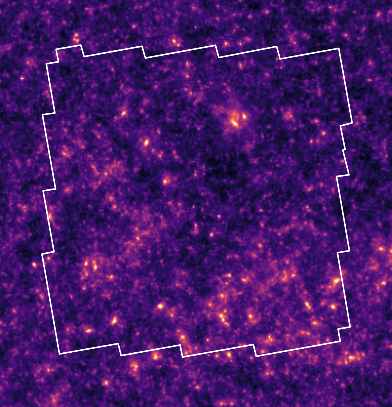
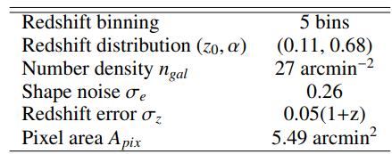
Mocked weak lensing maps
with sbi_lens
128x128x5 maps, spanning
10x10 deg²
LSST Y10-like survey setting
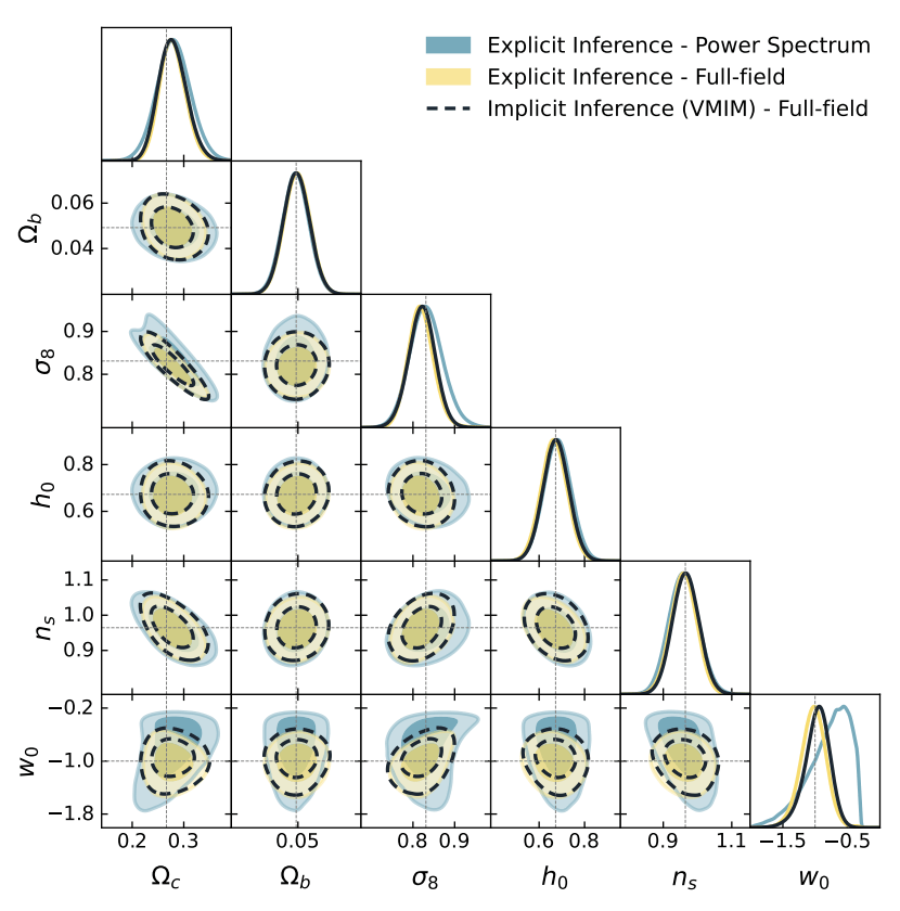
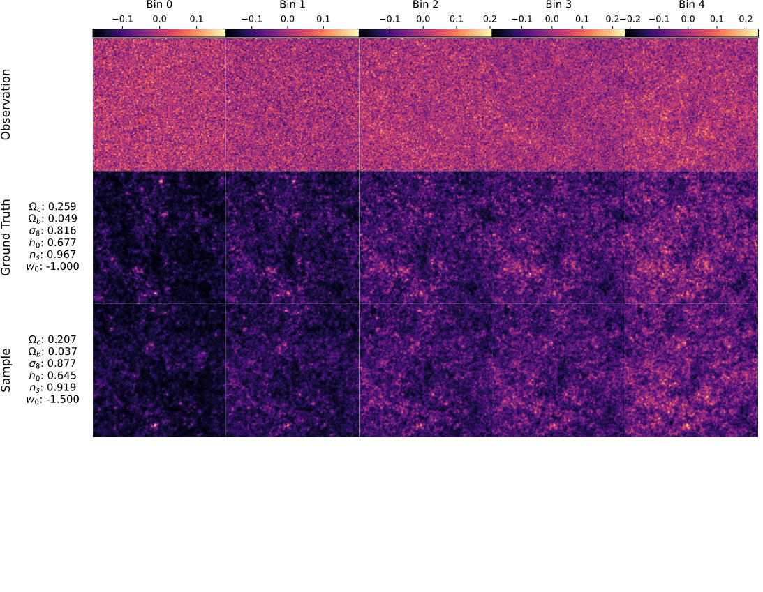
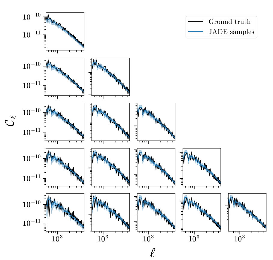
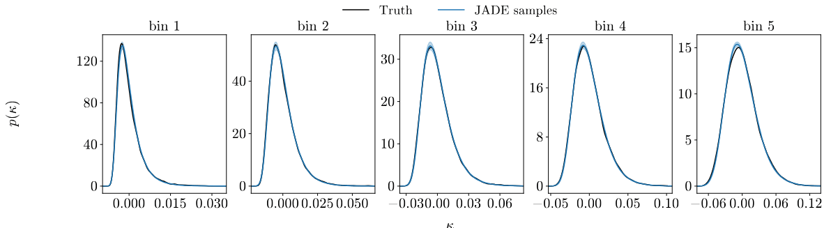
Results
Learning the joint distribution
p(\theta, \kappa)
Results
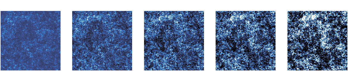
A fast and differentiable (JAX) log-normal mass maps simulator
sbi-lens
Learning the joint distribution
p(\theta, \kappa)
Results
Learning the joint distribution
p(\theta, \kappa)
Results
Learning the joint distribution
p(\theta, \kappa)
Results
Learning the joint distribution
p(\theta, \kappa)
Results
Learning the joint distribution
p(\theta, \kappa)
Results
Learning the joint distribution
p(\theta, \kappa)
Results
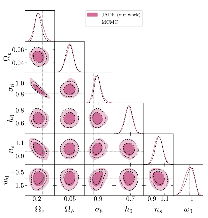
Cosmology marginal
p(\theta\mid \gamma)
TARP coverage test (Lemos et al. 2023)
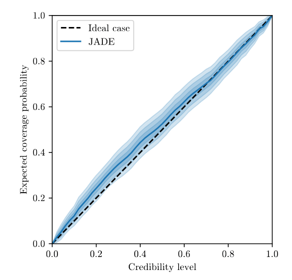
MIRA calibration score (Sharief, Zeghal, et al. 2026)
on the joint distribution, where 2/3 is optimal
0.6428 \pm 0.0149
Results
We built a generative model of mass-maps and cosmology, that we can condition on observation to get the joint posterior distribution
p(\theta, \kappa\mid \gamma)
Paper out this week!
Thank you!
This approach could be extended for inference, or to build efficient proposal, of initial condition and cosmology
Happy to chat about this!
\delta_\text{IC}, \theta \mid y_\text{obs}
Takeaways
PI-field-level
By Benjamin REMY


