Planning Through Contact with Trajectory Optimization and GCS
Robot Locomotion Group, MIT
Long Talk, Spring 2023
Bernhard Paus Græsdal
Why do we care about planning through contact?
-
Current systems are task-specific
-
We want a general planning framework for novel manipulation tasks
-
Combinatorial blowup and non-convexity makes motion planning a big challenge
Relevant Work
How is the problem solved today?
Typical tools of choice
1. Sampling-Based Planning
2. Trajectory Optimization
Russ Tedrake. Underactuated Robotics: Algorithms for Walking, Running, Swimming, Flying, and Manipulation (Course Notes for MIT 6.832)
Figures borrowed from:
1. Sampling-Based Manipulation Planning

Advantages
- Takes robot kinematics into account
- Doesn't explicitly reason about contact modes
Mode Sampling and projection onto contact manifold + RRT
Smooth dynamics + Reachability metric + RRT
Drawbacks
- Suffers the curse of dimensionality
- The "RRT"-dance
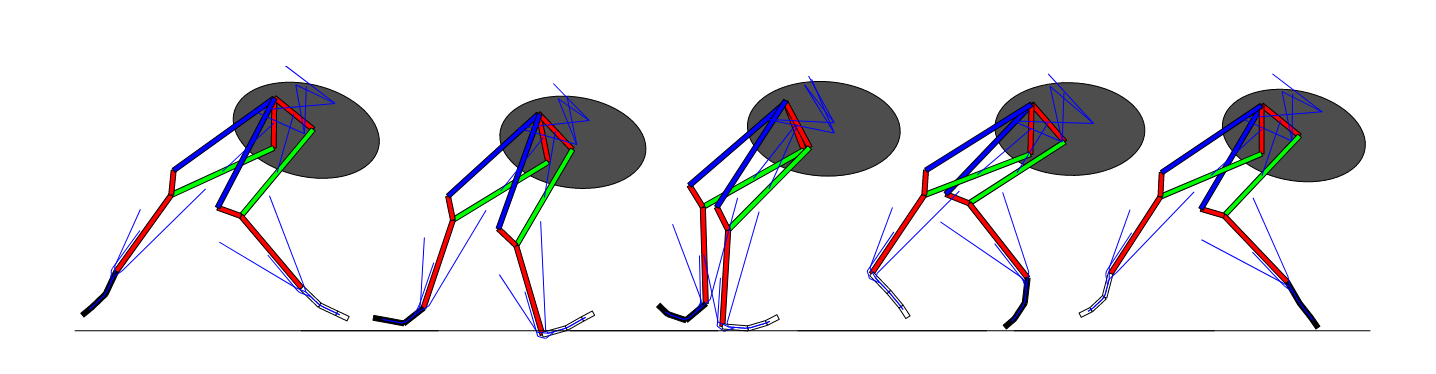
2. Contact-Rich Trajectory Optimization
Nonlinear optimization + Implicit contact modes (complimentarity condition)
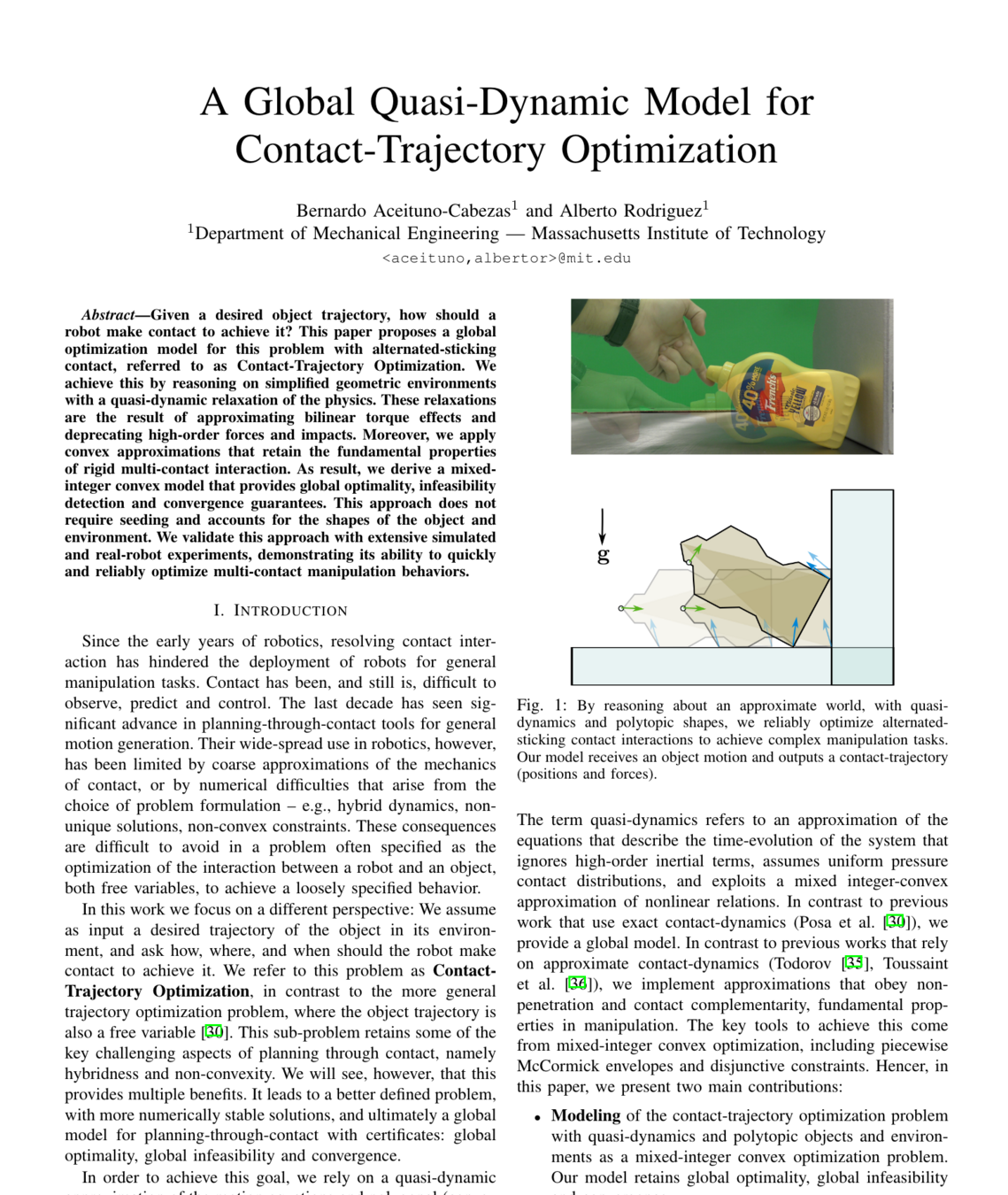
Mixed-Integer Convex Problem + Pre-specified trajectories + McCormick Relaxations
Advantages
- Works well with pre-defined mode schedules
(used a lot for locomotion) - (Local) optimality
Disadvantages
- Very hard when you also search over contact modes
- Non-convex in the general case with rotations
- For non-convex trajopt: reliant on initial guess and tuning
Sampling-Based Manipulation Planning
- Takes robot kinematics into account
- Doesn't explicitly reason about contact modes
- Suffers the curse of dimensionality
Smooth dynamics + Reachability metric + RRT
Sampling-Based Manipulation Planning
Mode Sampling and projection onto contact manifold + RRT
- TODO
Contact-Rich Trajectory Optimization
Nonlinear optimization + Implicit contact modes (complimentarity condition)
- Non-convex
- ??
- ??
Contact-Rich Trajectory Optimization
- Works well with pre-defined mode schedules
(used a lot for locomotion) - Hard when you search over contact modes
Nonlinear optimization + Implicit contact modes (complimentarity condition)
Contact-Rich Trajectory Optimization
Mixed-Integer Convex Problem + McCormick Relaxations
- Exponential in the number of contact modes
- Scales poorly
- TODO add videos?
Our Approach
Plan Through Contact Modes using GCS
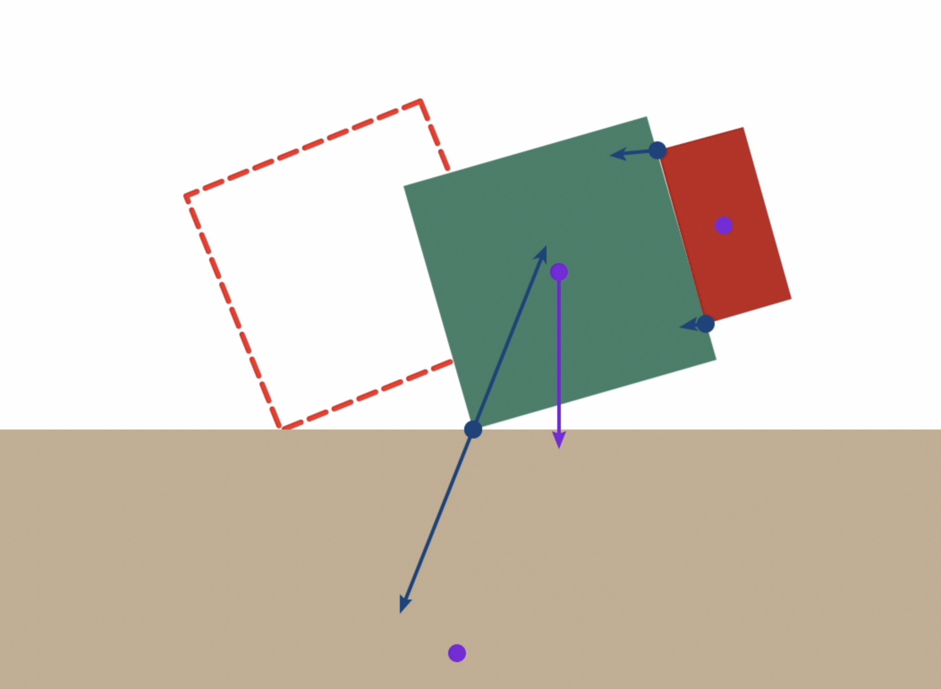
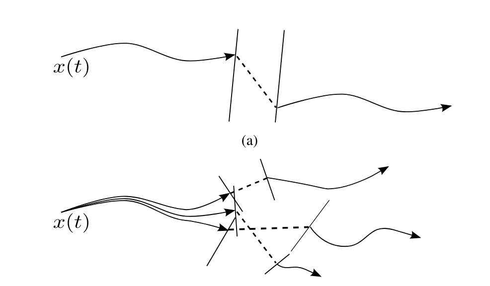
How to flip up and push the object?
To plan this motion, we need to simultaneously decide:
- Contact mode sequence
- Continuous motion within each contact mode
Motivational Example
[1] N. Doshi, O. Taylor, and A. Rodriguez, “Manipulation of unknown objects via contact configuration regulation.” arXiv, Jun. 01, 2022. doi: 10.48550/arXiv.2203.01203.
Figure taken from [1]
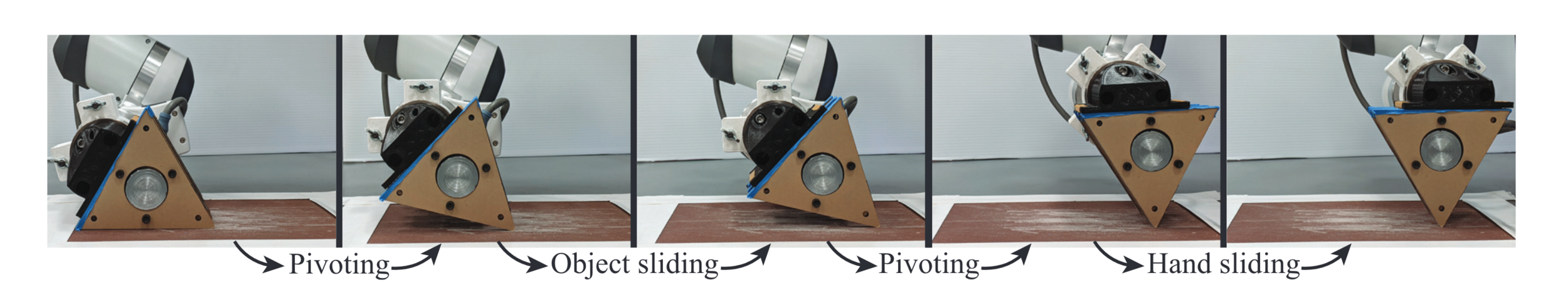
The task at hand
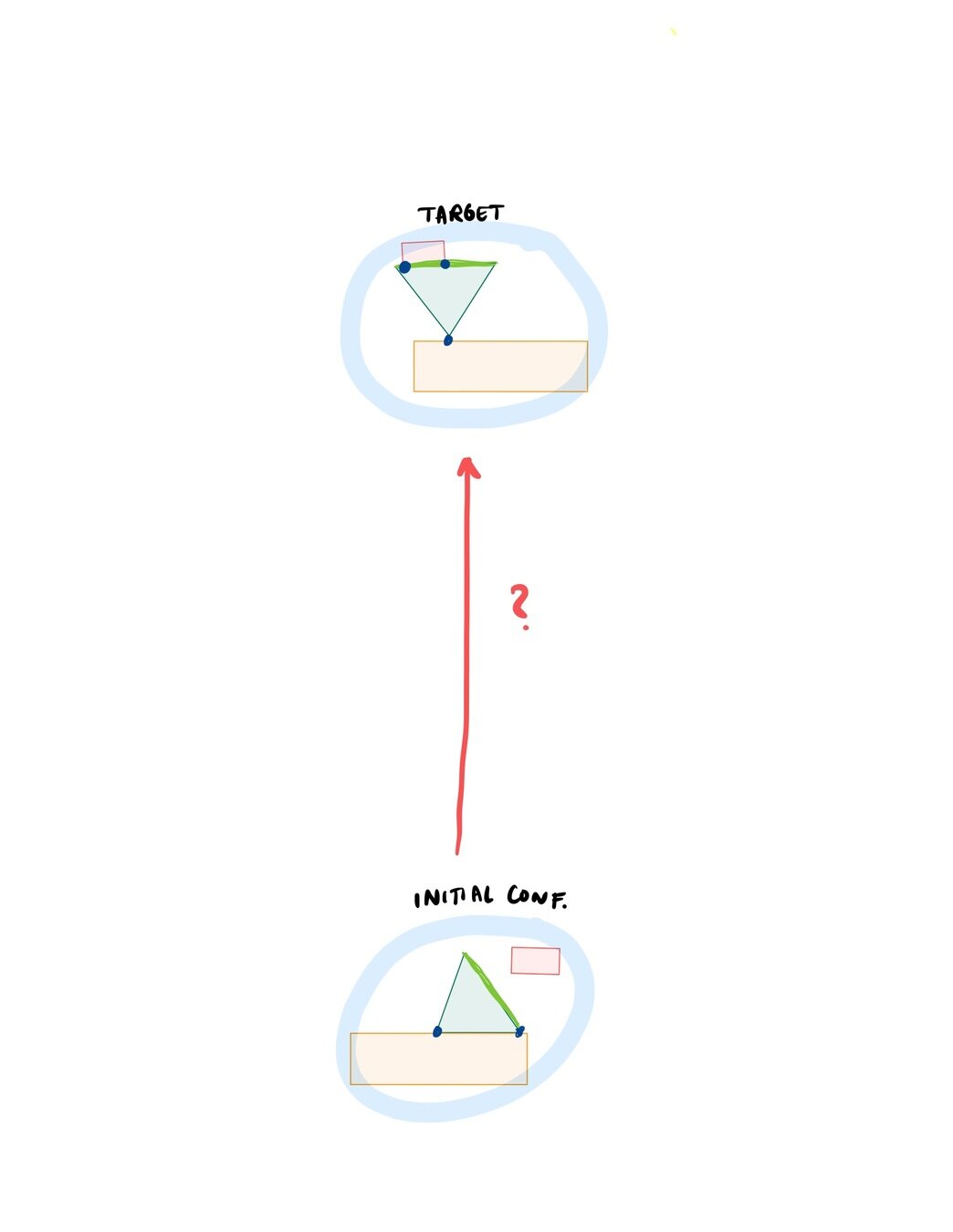
We want to...
- Flip up the object
- Push the object
- Reposition the end-effector
... in no particular order
While minimizing some quantity:
- Kinetic energy
- Exerted work
- ...
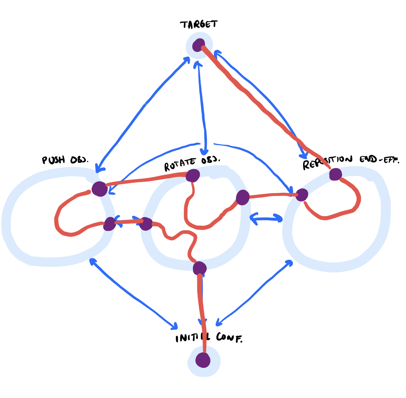
Let's build a graph
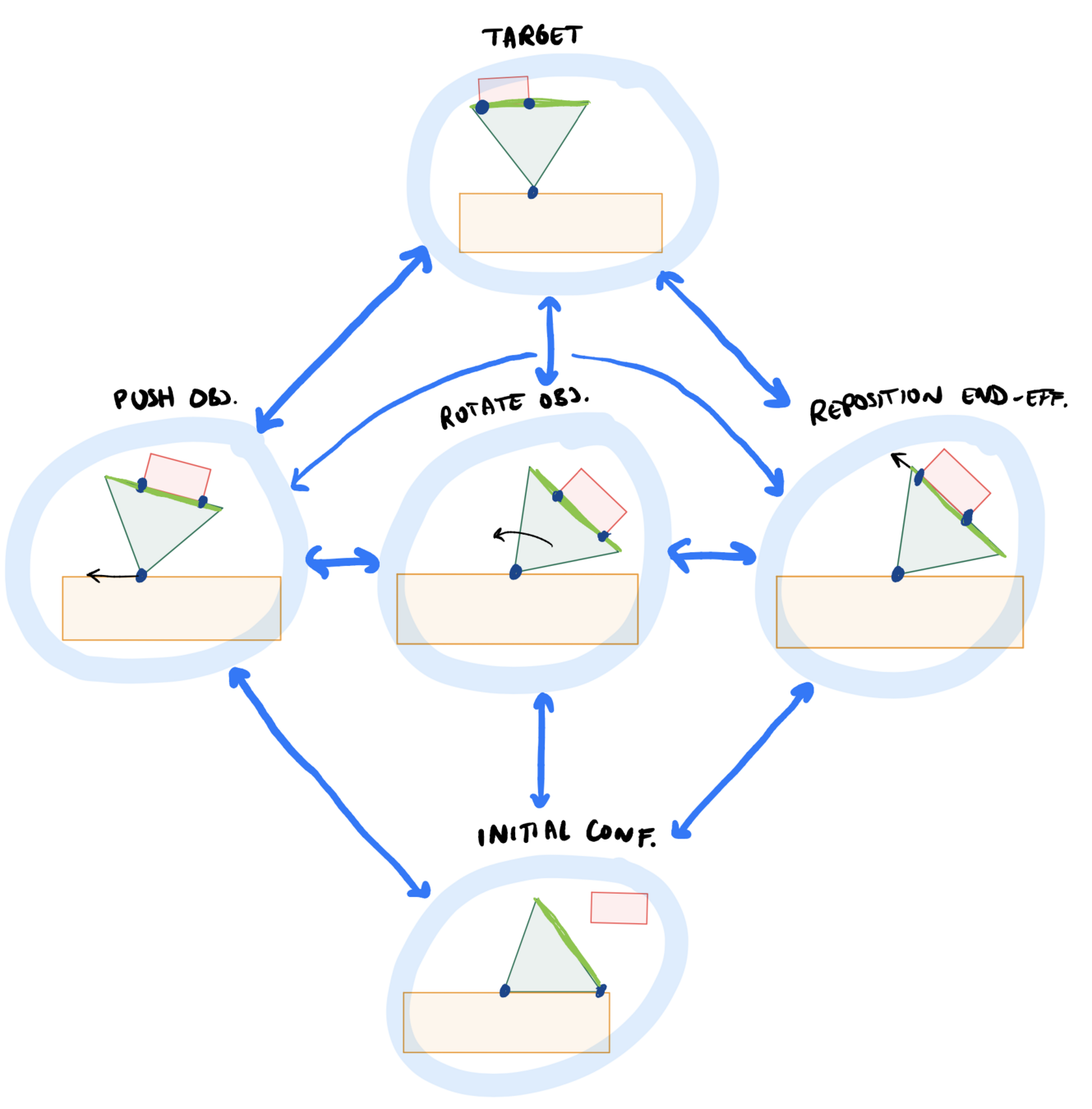
- Each contact mode is a set!
- Initial and target configurations are singletons
Let's build a graph
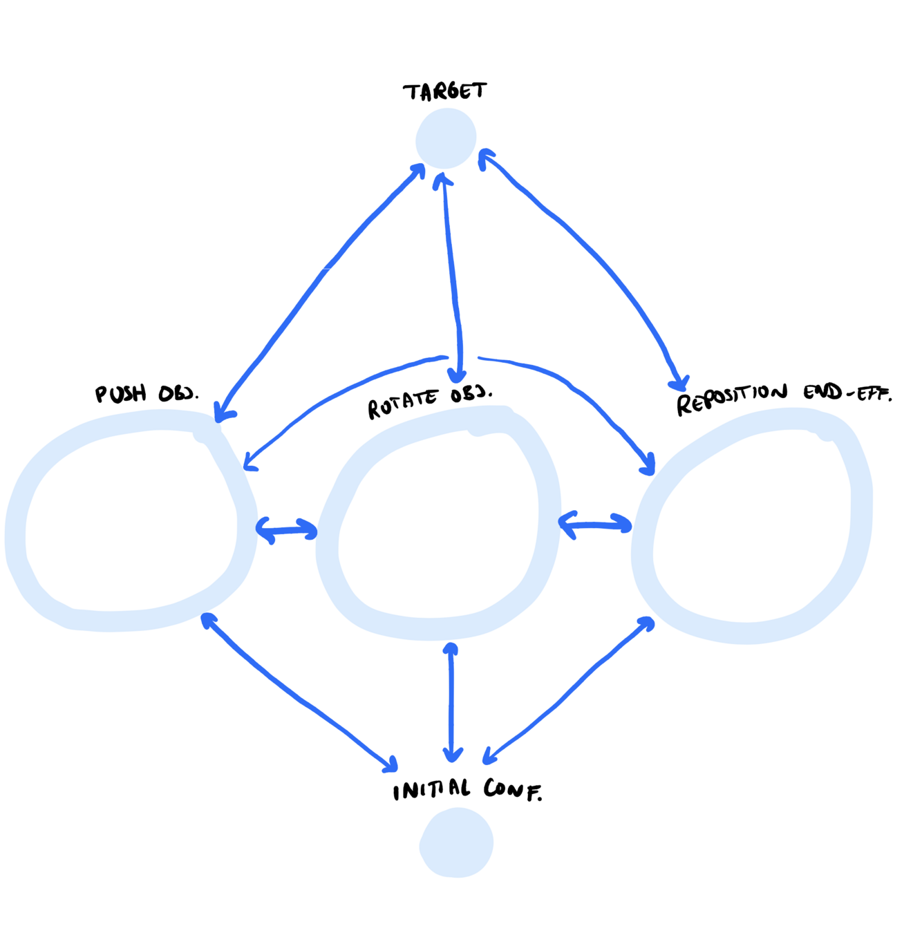
- More abstractly, we get a graph like this:
Let's build a graph
If we can solve the SPP, we have our plan!
\Updownarrow
Our Approach
+
Plan through contact using GCS
\implies
- Sets are contact modes
There's a problem with this picture...
Can we plan through contact modes with GCS?
Generally, no!
- Contact modes are non-convex
- However, the sets are basic semi-algebraic!
We need to find a convex formulation (relaxation) for the contact modes
Preliminary Results
Planning within one contact mode
Object Flip-Ups & Pushing
Object Flip-Ups
Planar Pushing
Planning Through Contact Modes with GCS
(In the convex, non-rotational case)
Problem Formulation
Problem Formulation
Making the contact modes convex
Contact Modelling
Modelling Choices
Modelling decisions (1/2):
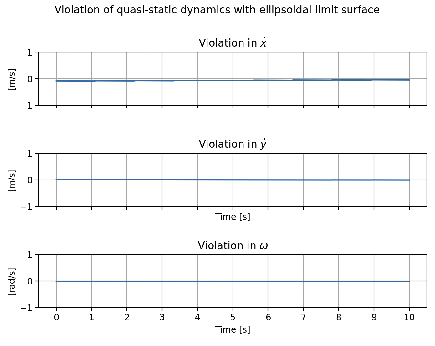
- Assume quasi-static dynamics:
- Low velocities, low inertial forces and no impacts
- Low velocities, low inertial forces and no impacts
- (Quasi-dynamic: Allows brief periods of dynamic motion, but assumes accelerations do not integrate into significant velocities)
\begin{aligned}
M (q) \dot{{v}} + {C} (q, v) v = &\tau_g(q) + \sum_i J_{c,i}^\intercal f^{c_i} \\
M (q) \dot{{v}} + {C} (q, v) v \approx 0
\implies
&\tau_g(q) + \sum_i J_{c,i}^\intercal f^{c_i} = 0
\end{aligned}
Modelling Choices
Modelling decisions (2/2)
- Use relative quantities in frames of objects in contact
- Minimize kinetic energy
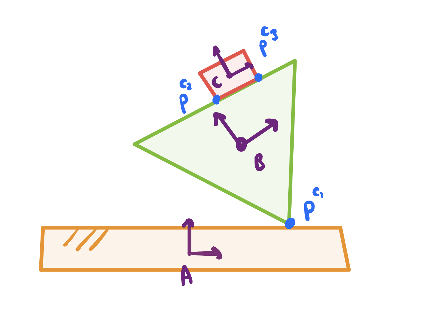
Defining Decision Variables
- Relative positions
- Relative rotation
- Contact positions (in local frames)
- Contact forces
{}^A p^B, {}^B p^A \in \mathbb{R}^2
{}^A R^B \in SO(2)
(A,B)
For each active contact pair
{}p^{c_i}_A, \, {}p^{c_i}_B \in \mathbb{R}^2 \quad \\
f^{c_i}_A, f^{c_i}_B \in \mathbb{R}^2
\\ \quad \quad \forall i \in \text{Contact points}
For each knot point \( k = 0, \ldots , N \)
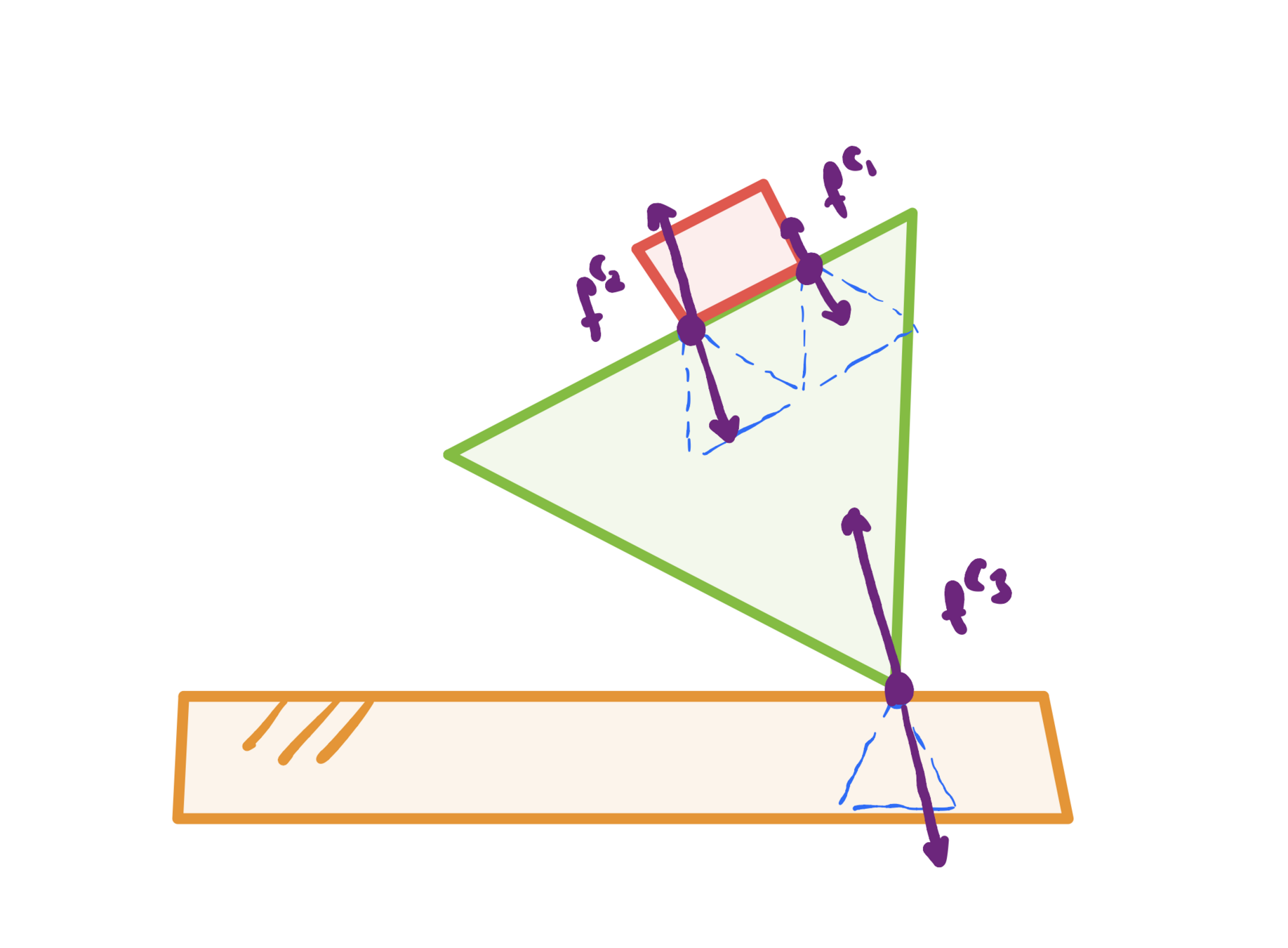
Consistency across frames
- Contact points equal
- Relative positions consistent
- Newton's third law for contact forces
- where \(W\) is some common frame
[{}^{{A}} p^{c_i}]_{{W}}
=
[{}^{{B}} p^{c_i}]_{{W}}
(A,B)
For each active contact pair
[{}^{{A}} p^{B}]_{{W}}
=
-
[{}^{{B}} p^{A}]_{{W}}
[
{f}^{c_i}_{{A}}
]_{{W}}
=
-[
{f}^{c_i}_{{B}}
]_{{W}}.
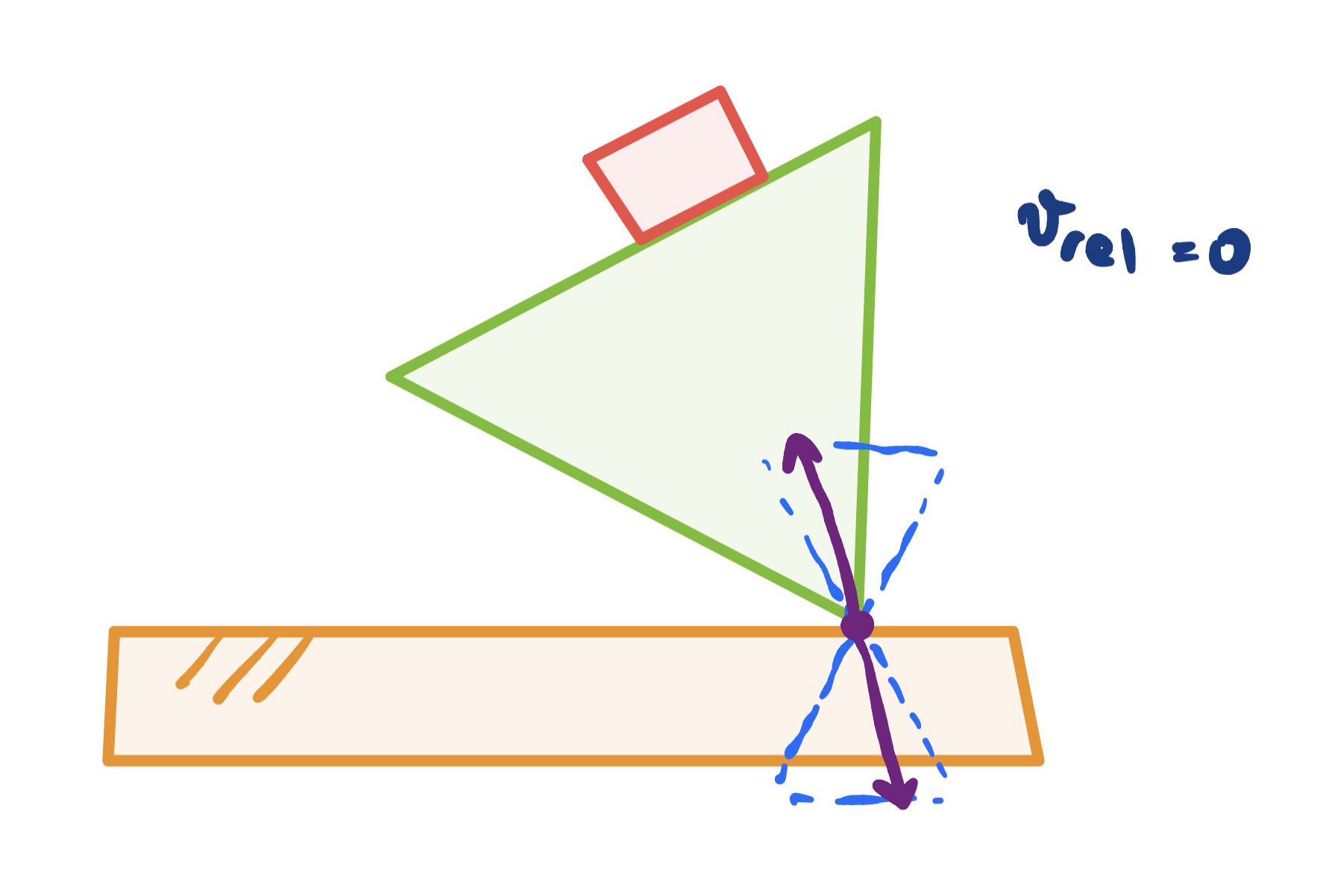
Contact modes
\begin{aligned}
c^{n_i} &\geq 0 \\
\left| c^{f_i} \right| &\leq \mu c^{n_i} \\
v_{\text{rel}} &= 0
\end{aligned}
- Sticking contact
\begin{aligned}
c^{n_i} &\geq 0 \\
\left| c^{f_i} \right| &= \mu c^{n_i} \\
v_{\text{rel}} &\geq 0 \quad \text{or} \quad
v_{\text{rel}} \leq 0
\end{aligned}
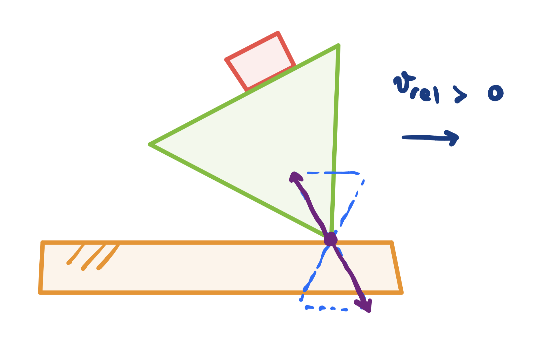
2. Sliding contact
All constraints
\begin{aligned}
\quad
\tau_g(q) + \sum_i J_{c,i}^\intercal f^{c_i} &= 0 \\
\quad
{}^A R^B &\in SO(2), \\
\quad
f^{c_i} &\in \mathcal{FC}_i \\
\quad
p^{c_i} &\in \text{Face} \, \text{or} \, \text{Vertex} \\
M R &\geq 0 \quad (\text{non-penetration}) \\
\quad
[{}^{{A}} p^{c_i}]_{{W}}
&=
[{}^{{B}} p^{c_i}]_{{W}} \\
\quad
[{}^{{A}} p^{B}]_{{W}}
&=
-
[{}^{{B}} p^{A}]_{{W}} \\
\quad
[
{f}^{c_i}_{{A}}
]_{{W}}
&=
-[
{f}^{c_i}_{{B}}
]_{{W}} \\
\quad \forall (A,B) &\in \text{Contact Pairs} \\
\quad \forall i &\in \text{Contact Points}
\end{aligned}
(for planning within one contact mode)
Non-convex
(quadratic equality constraints)
(knot point indices omitted for notational simplicity)
Cost
- We assume low velocities
- \( \implies \) Minimize kinetic energy over the trajectory
\begin{aligned}
K &= \int_0^T \left[ \frac{1}{2}m \lVert v (t) \rVert^2 + \frac{1}{2} I \lVert \omega (t) \rVert ^2 \right] dt
\end{aligned}
- \( v(t) = \dot p(t) \)
- In general \( [\omega]^\times = \dot R R ^ \intercal \). We obtain \( \lVert \omega \rVert ^2 \) as
\begin{aligned}
\lVert \omega (t) \rVert ^2 =
\omega ^\intercal \omega
=
\frac{1}{2} \text{vec}(\dot R)^\intercal
\text{vec}(\dot R)
&:= \frac{1}{2} \lVert \dot r(t) \rVert^2
\\
r &:= \text{vec}(R)
\end{aligned}
(Proof on next slide)
\begin{aligned}
\implies
K
&= \int_0^T \left[ \frac{1}{2}m \dot p(t)^\intercal \dot p(t) + \frac{1}{4} I \dot r(t)^\intercal \dot r(t) \right] dt
\end{aligned}
Cost
(Proof):
\begin{aligned}
\implies
\lVert \omega \rVert ^2 =
\omega ^\intercal \omega
&=
\frac{1}{2}
\text{Tr}([\omega]^\times {}^\intercal [\omega]^\times)
= \frac{1}{2}\text{Tr}(R \dot R^\intercal \dot R R^\intercal) \\
&= \frac{1}{2} \text{Tr}(\dot R^\intercal \dot R)
=
\frac{1}{2} \text{vec}(\dot R)^\intercal
\text{vec}(\dot R) \\
&:= \frac{1}{2} \dot r^\intercal \dot r = \frac{1}{2} \lVert \dot r \rVert^2 \quad \quad \square
\end{aligned}
\frac{1}{2} \text{Tr}([a]^\times {}^\intercal [a]^\times)
=
\text{vec}(a)^\intercal
\text{vec}(a)
= a^\intercal a
[\omega]^\times = \dot R R ^ \intercal
\text{Tr}(A^\intercal B)
=
\text{vec}(A)^\intercal
\text{vec}(B)
Cost
\begin{aligned}
K
&= \int_0^T \left[ \frac{1}{2}m \dot p(t)^\intercal \dot p(t) + \frac{1}{4} I \dot r(t)^\intercal \dot r(t) \right] dt
\end{aligned}
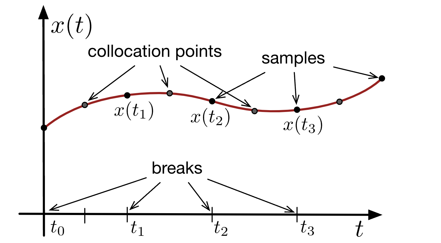
- Use forward-differences to obtain derivatives
v[i] = \dot p[i] := \frac{1}{\Delta t} (p[i+1] - p[i])
- Use Riemann-sums to approximate the integral
- We thus minimize the following cost:
\begin{aligned}
K
&\approx
\sum_{k=0}^{N}
k_v
(p_{k+1} - p_{k})^\intercal
(p_{k+1} - p_{k})
+
k_\omega
(r_{k+1} - r_{k})^\intercal
(r_{k+1} - r_{k})
\end{aligned}
Cost Summary
\begin{aligned}
K &= \int_0^T \left[ \frac{1}{2}m \lVert v (t) \rVert ^2 + \frac{1}{2} I \lVert \omega(t) \rVert^2 \right] dt \\
&= \int_0^T \left[ \frac{1}{2}m \dot p(t)^\intercal \dot p(t) + \frac{1}{4} I \dot r(t)^\intercal \dot r(t) \right] dt \\
&\approx
\sum_{k=0}^{N}
k_v
\lVert p_{k+1} - p_{k} \rVert^2
+
k_\omega
\lVert r_{k+1} - r_{k} \rVert^2
\end{aligned}
Minimizing kinetic energy of the trajectory
\( \Updownarrow \)
Minimizing squared Euclidean distances directly in the coordinates of the position and rotation
Full Optimization Problem
\begin{aligned}
\min_{p, p^{c_i}, f^{c_i}, R}
\quad
\sum_{k=0}^{N}
k_v
\lVert p_{k+1} - p_{k} \rVert^2
&+
k_\omega
\lVert r_{k+1} - r_{k} \rVert^2 \\
\text{subject to}
\quad
\tau_g(q) + \sum_i J_{c,i}^\intercal f^{c_i} &= 0 \\
\quad
{}^A R^B &\in SO(2), \\
\quad
f^{c_i} &\in \mathcal{FC}_i \\
\quad
p^{c_i} &\in \text{Face} \, \text{or} \, \text{Vertex} \\
M R &\geq 0 \quad (\text{non-penetration}) \\
\quad
[{}^{{A}} p^{c_i}]_{{W}}
&=
[{}^{{B}} p^{c_i}]_{{W}} \\
\quad
[{}^{{A}} p^{B}]_{{W}}
&=
-
[{}^{{B}} p^{A}]_{{W}} \\
\quad
[
{f}^{c_i}_{{A}}
]_{{W}}
&=
-[
{f}^{c_i}_{{B}}
]_{{W}} \\
\quad \forall (A,B) &\in \text{Contact Pairs} \\
\quad \forall i &\in \text{Contact Points}
\end{aligned}
(for planning within one contact mode)
Non-convex
(quadratic equality constraints)
(knot point indices omitted for notational simplicity)
Full Optimization Problem
- The feasible set is a basic semi-algebraic set
$$\left\{ f_i(x) = 0, \, g_i(x) \geq 0 \right\}$$ i.e. described by finitely many polynomial constraints.
-
Moreover, it is described by second order polynomials
-
Cost is also quadratic
\begin{aligned}
\min_{p, p^{c_i}, f^{c_i}, R}
\quad
\sum_{k=0}^{N}
k_v
\lVert p_{k+1} - p_{k} \rVert^2
&+
k_\omega
\lVert r_{k+1} - r_{k} \rVert^2 \\
\text{subject to}
\quad
\tau_g(q) + \sum_i J_{c,i}^\intercal f^{c_i} &= 0 \\
\quad
{}^A R^B &\in SO(2), \\
\quad
f^{c_i} &\in \mathcal{FC}_i \\
\quad
p^{c_i} &\in \text{Face} \, \text{or} \, \text{Vertex} \\
M R &\geq 0 \quad (\text{non-penetration}) \\
\quad
[{}^{{A}} p^{c_i}]_{{W}}
&=
[{}^{{B}} p^{c_i}]_{{W}} \\
\quad
[{}^{{A}} p^{B}]_{{W}}
&=
-
[{}^{{B}} p^{A}]_{{W}} \\
\quad
[
{f}^{c_i}_{{A}}
]_{{W}}
&=
-[
{f}^{c_i}_{{B}}
]_{{W}} \\
\quad \forall (A,B) &\in \text{Contact Pairs} \\
\quad \forall i &\in \text{Contact Points}
\end{aligned}
(for planning within one contact mode)
Full Optimization Problem
\begin{aligned}
\min_{x} \quad x^\intercal Q_0 x & \\
\text{subject to}
\quad
x^\intercal Q_i x &\geq 0, \quad \forall i = 1, \ldots \\
\quad
Ax &\geq 0 \\
\quad
x &=
\begin{bmatrix}
1 \\
y
\end{bmatrix}
\end{aligned}
- The problem is naturally a (non-convex) QCQP
Solving it: SDP Relaxation
\begin{aligned}
\min_{x} \quad x^\intercal Q_0 x & \\
\text{subject to}
\quad
x^\intercal Q_i x &\geq 0, \quad \forall i = 1, \ldots \\
\quad
Ax &\geq 0 \\
\quad
x &=
\begin{bmatrix}
1 \\
y
\end{bmatrix}
\end{aligned}
- We solve it with the standard SDP relaxation
\begin{aligned}
\min_{x} \quad \langle Q_0, X \rangle & \\
\text{subject to}
\quad
\langle Q_i, X \rangle &\geq 0, \quad \forall i = 1, \ldots \\
\quad
AXA^\intercal &\geq 0 \\
\quad
AXe_1^\intercal &\geq 0 \\
\quad
e_1^\intercal X e_1 &= 1 \\
\quad
X \succeq 0 \\
\end{aligned}
\( \longrightarrow \)
- Exact when \( \text{rank}(X) = 1 \iff X = x x^\intercal \)
- (This includes the McCormick envelope/outer-approximation of bilinear constraints)
- Now we have a convex set!
\( X := xx^\intercal \)
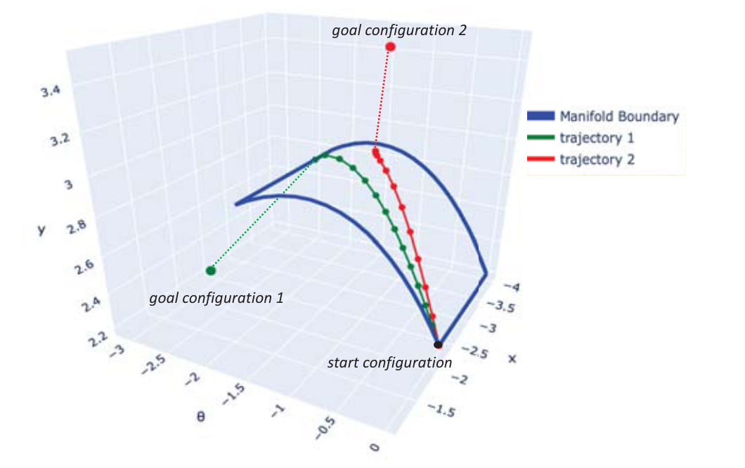
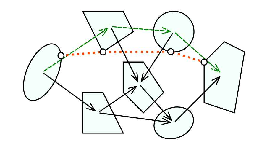
Minimizing kinetic energy makes the SO(2) relaxation tight
\begin{aligned}
\min_{x_k \in \mathbb{R}^2}
\quad &
\sum^{d-1}_{k = 0}
(x_{k+1} - x_{k})^\intercal
(x_{k+1} - x_{k}) \\
\textrm{s.t.}
\quad &
x_k^\intercal x_k = 1
\quad k = 0, \ldots, d \\
\quad & x_0 = \bar x_I \\
\quad & x_d = \bar x_F \\
\end{aligned}
- Formulate the following minimal problem
- Solving the relaxed problem gives the true solution!
- We expect this to also hold for SO(3)
- (A formal tightness proof using the dual of the relaxation is in the works)
\begin{aligned}
x_k &=
\begin{bmatrix}
\cos\theta_k \\
\sin\theta_k \\
\end{bmatrix} \\
&:=
\begin{bmatrix}
c_k \\
s_k
\end{bmatrix},
\quad k = 0, \ldots, d
\end{aligned}
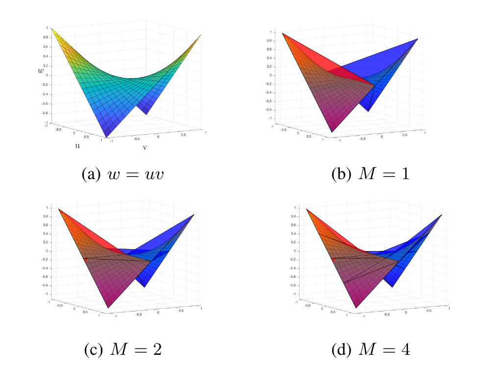
Minimizing kinetic energy makes the SO(2) relaxation tight
- Naive SOCP relaxation
\( c_\theta^2 + s_\theta^2 \leq 1 \)
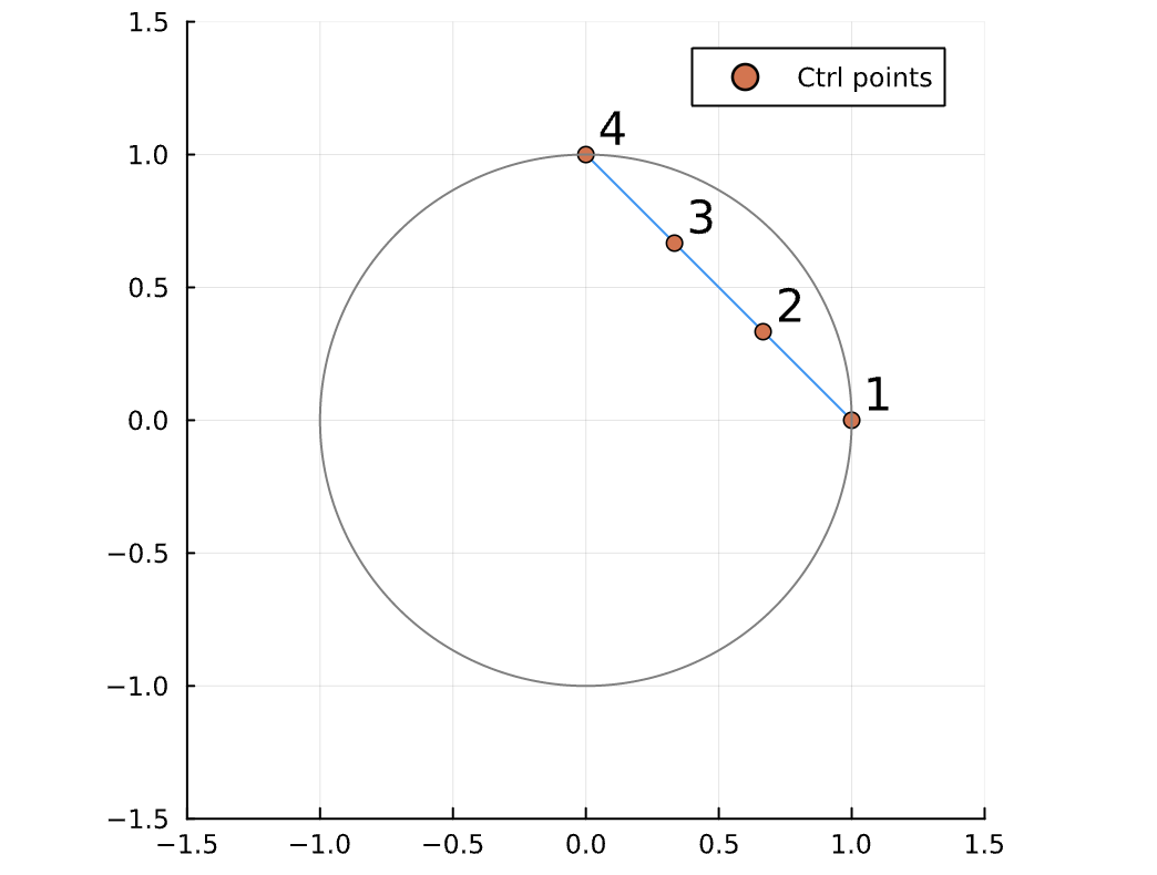
- SDP relaxation
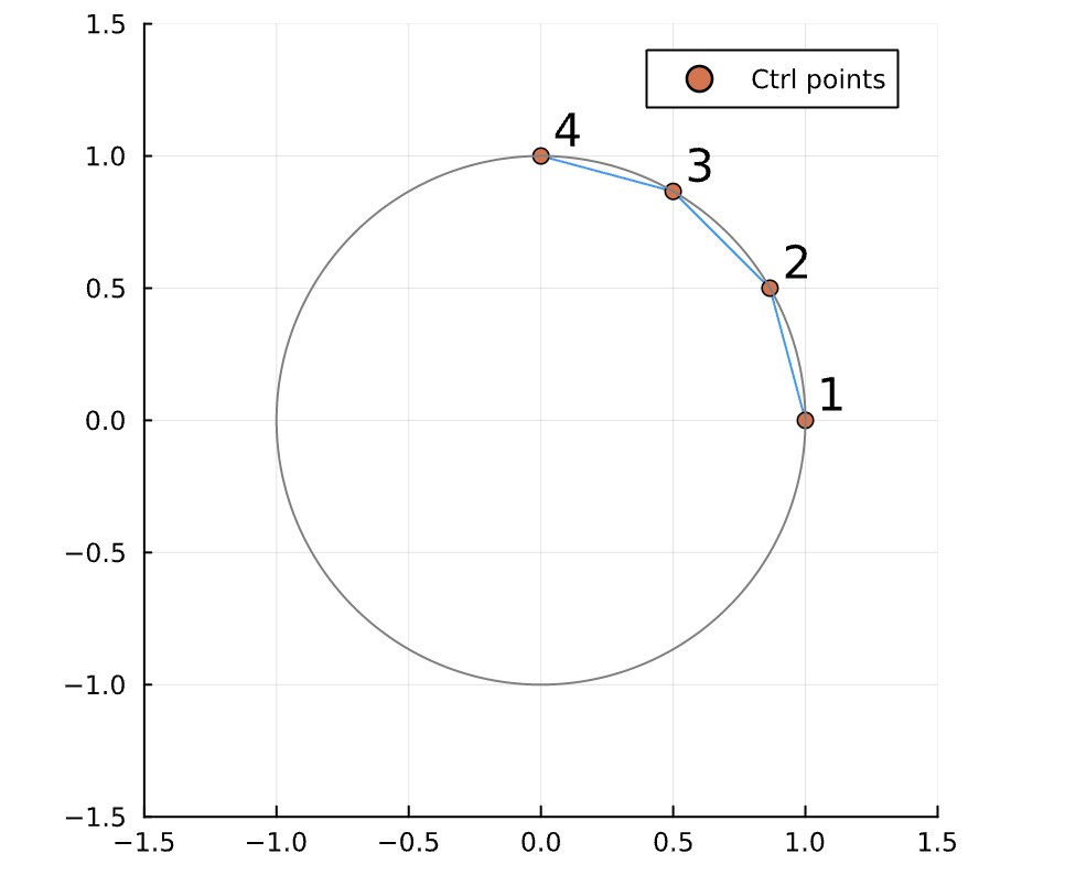
(Points 1 and 4 are fixed from boundary conditions)
Results
Making the contact modes convex
Object Flip-Ups & Pushing
Tightness Results
Pentagon
Mass: 1kg
COM to vertex: 0.2 m
"Reference force" = \( mg \approx 10 N \)
Object Flip-Ups & Pushing
Tightness Results
Box
Mass: 1kg
COM to vertex: 0.2 m
"Reference force" = \( mg \approx 10 N \)
Object Flip-Ups & Pushing
Tightness Results
Worst case: Triangle
Mass: 1kg
COM to vertex: 0.2 m
"Reference force" = \( mg \approx 10 N \)
Object Flip-Ups & Pushing
Tightness Results
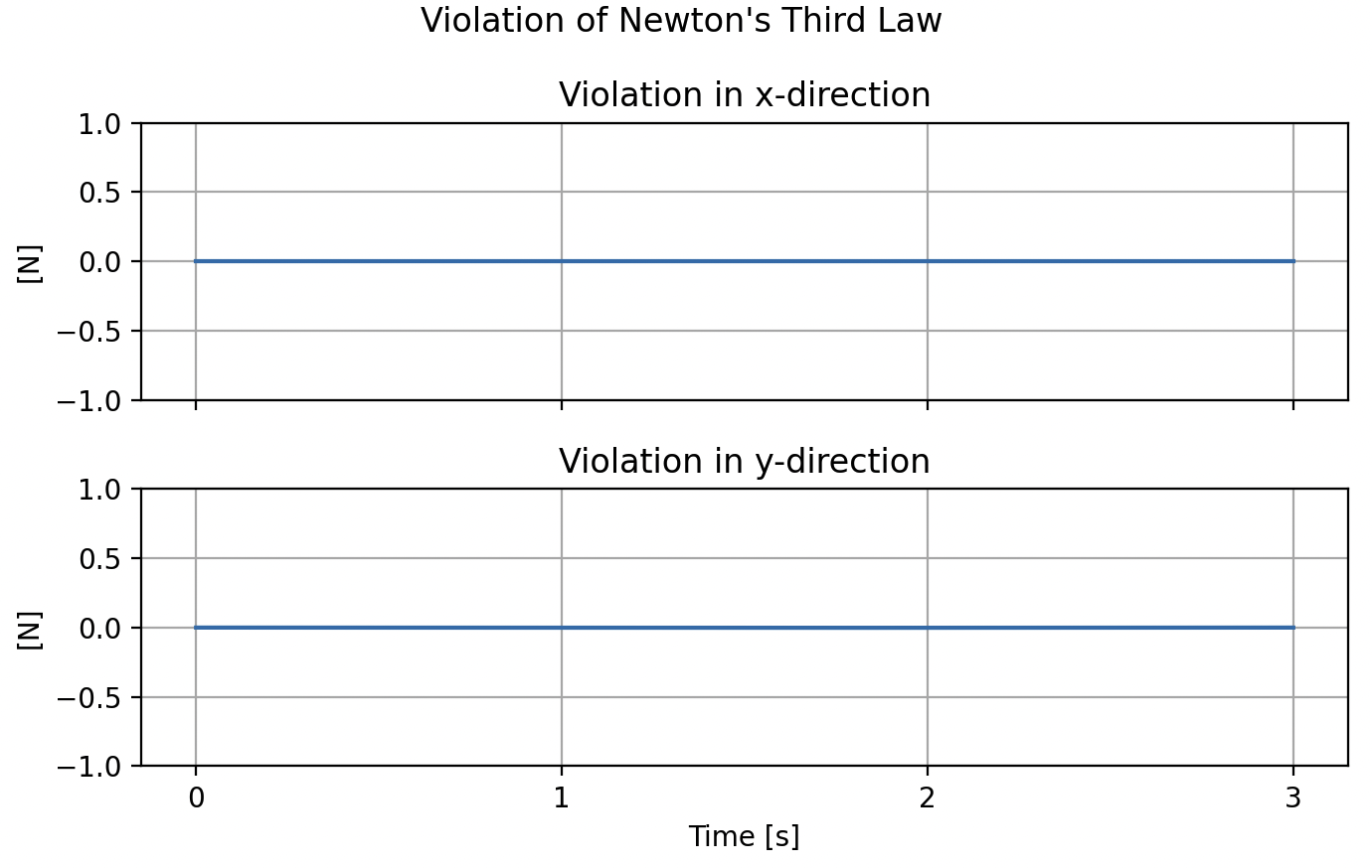
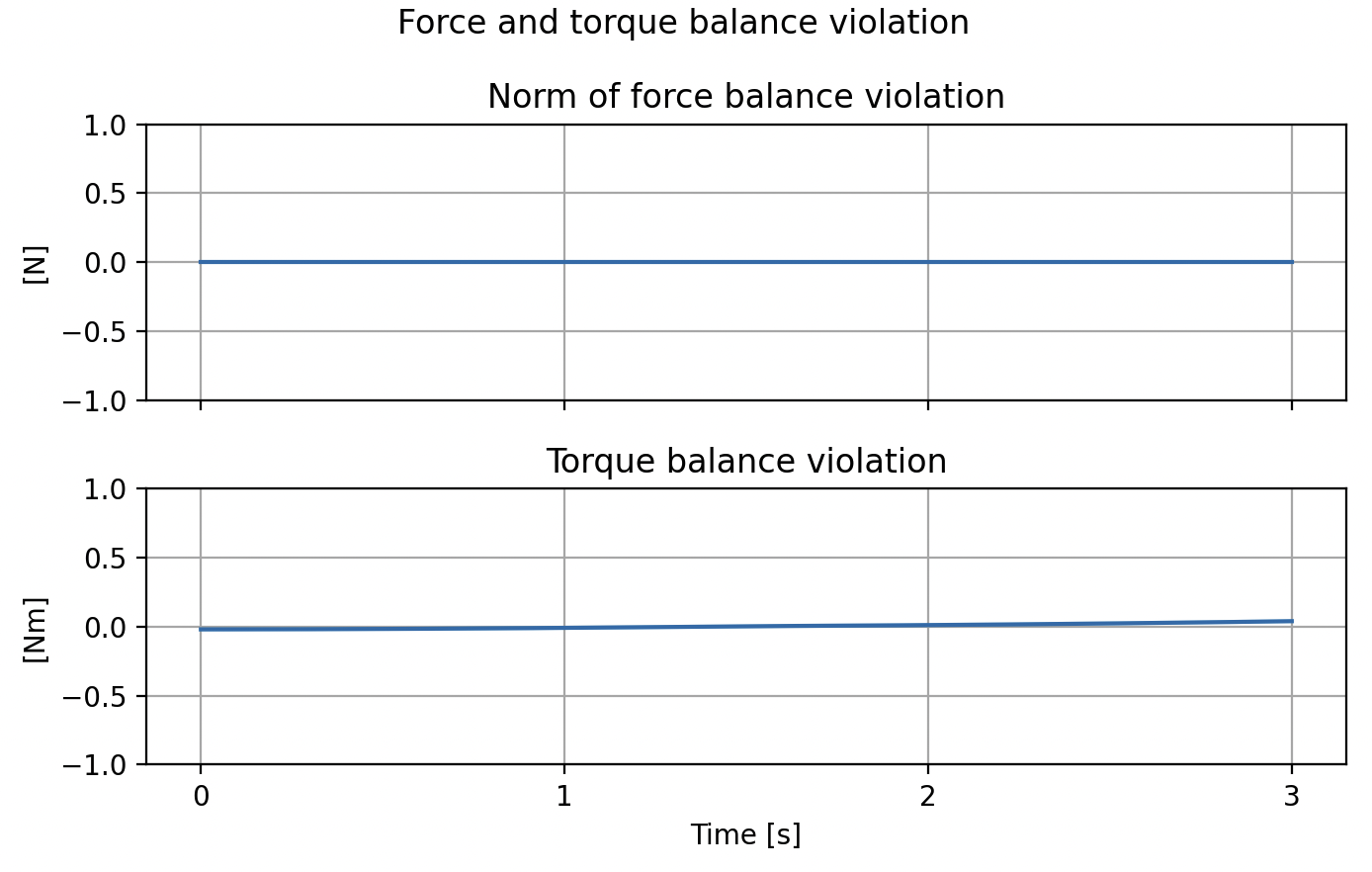
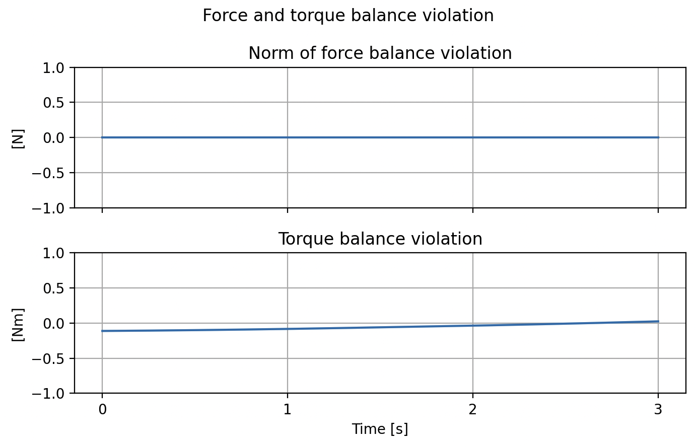
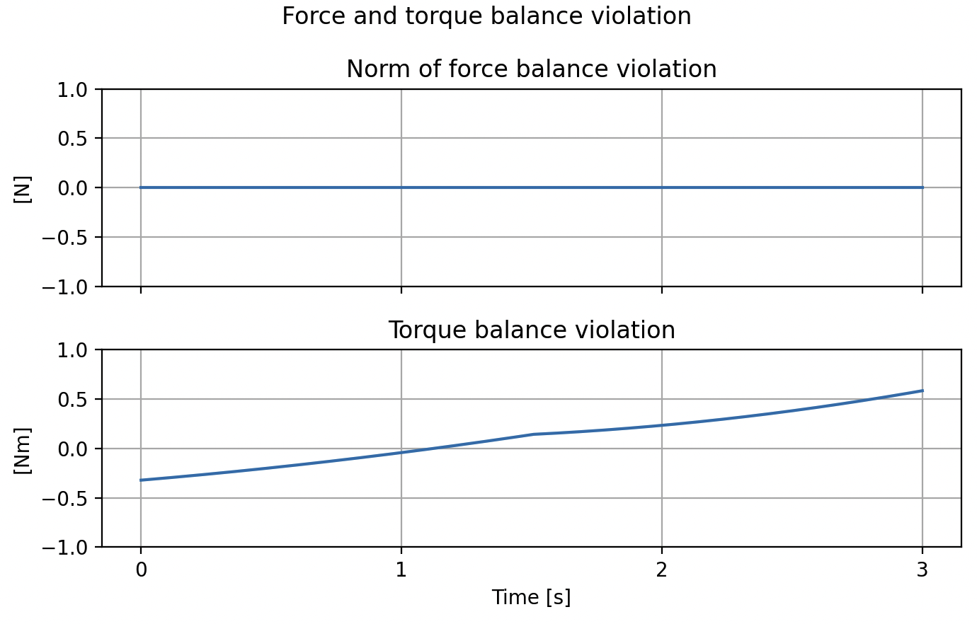
Preliminary Conclusions
- SO(2) relaxation is tight
\( \implies \) Force balance is tight - Sometimes (small) violation of torque balance
- For certain initial conditions, Newton's third law gets violated
(we suspect this is for infeasible initial conditions)
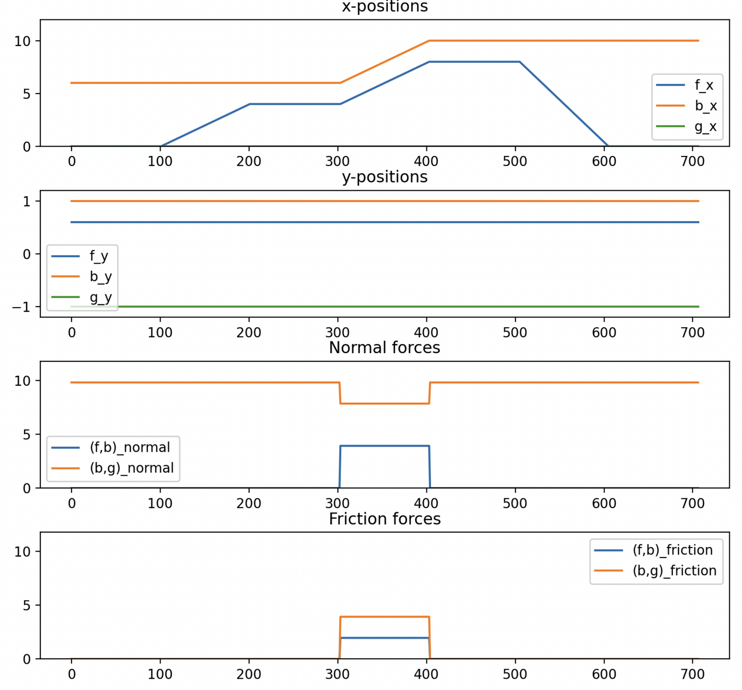
Planar Pushing
Tightness Results
For triangle:
- Similar for all shapes
- Preliminary analysis: Seems to be tight
Future/planned work
- Use GCS to plan through contact modes
- Stabilize trajectories in simulation
- Extend to the 3D case
- Longer-term: Work on dealing with contact mode explosion
Planning Through Contact Using Trajectory Optimization and GCS
By Bernhard Paus Græsdal


