Soss: Lightweight Probabilistic Programming in Julia
Chad Scherrer
Senior Data Scientist, Metis
GLOBAL BIG DATA
CONFERENCE
About Me
Served as Technical Lead for language evaluation for the DARPA program
Probabilistic Programming for Advancing Machine Learning (PPAML)
PPL Publications
-
Scherrer, Diatchki, Erkök, & Sottile, Passage : A Parallel Sampler Generator for Hierarchical Bayesian Modeling, NIPS 2012 Workshop on Probabilistic Programming
-
Scherrer, An Exponential Family Basis for Probabilistic Programming, POPL 2017 Workshop on Probabilistic Programming Semantics
- Westbrook, Scherrer, Collins, and Mertens, GraPPa: Spanning the Expressivity vs. Efficiency Continuum, POPL 2017 Workshop on Probabilistic Programming Semantics
Making Rational Decisions
Managed Uncertainty
Rational Decisions
Bayesian Analysis
Probabilistic Programming
- Physical systems
- Hypothesis testing
- Modeling as simulation
- Medicine
- Finance
- Insurance
Risk
Custom models


Business Applications
Missing Data
The Two-Language Problem
A disconnect between the "user language" and "developer language"
X
3
Python
C
Deep Learning Framework
- Harder for beginner users
- Barrier to entry for developers
- Limits extensibility
?
A New Approach in Julia
- Models begin with "Tilde code" based on math notation
- A Model is a "lossless" data structure
-
Combinators transform code before compilation
Model
Tilde code
\begin{aligned}
\mu &\sim \text{Normal}(0,5)\\
\sigma &\sim \text{Cauchy}_+(0,3) \\
x_j &\sim \text{Normal}(\mu,\sigma)
\end{aligned}
Advantages
- Transparent
- Composable
- Backend-agnostic
- No intrinsic overhead
A (Very) Simple Example
P(\mu,\sigma|x)\propto P(\mu,\sigma)P(x|\mu,\sigma)
\begin{aligned}
\mu &\sim \text{Normal}(0,5)\\
\sigma &\sim \text{Cauchy}_+(0,3) \\
x_j &\sim \text{Normal}(\mu,\sigma)
\end{aligned}
m = @model N begin
    μ ~ Normal(0, 5)
    σ ~ HalfCauchy(3)
    x ~ Normal(μ, σ) |> iid(N)
end
Theory
Soss
julia> sourceLogdensity(m)
:(function ##logdensity#1168(pars)
      @unpack (μ, σ, x, N) = pars
      ℓ = 0.0
      ℓ += logpdf(Normal(0, 5), μ)
      ℓ += logpdf(HalfCauchy(3), σ)
      ℓ += logpdf(Normal(μ, σ) |> iid(N), x)
      return ℓ
  end)
A (Slightly Less) Simple Example
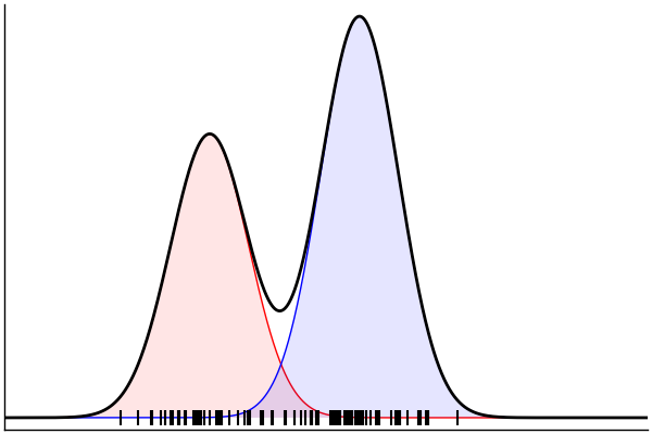
gaussianMixture = @model begin
    N ~ Poisson(100)
    K ~ Poisson(2.5)
    p ~ Dirichlet(K, 1.0)
    μ ~ Normal(0,1.5) |> iid(K)
    σ ~ HalfNormal(1)
    θ = [(m,σ) for m in μ]
    x ~ MixtureModel(Normal, θ, p) |> iid(N)
end
julia> m = gaussianMixture(N=100,K=2)
@model begin
    p ~ Dirichlet(2, 1.0)
    μ ~ Normal(0, 1.5) |> iid(2)
    σ ~ HalfNormal(1)
    θ = [(m,σ) for m in μ]
    x ~ MixtureModel(Normal, θ, p) |> iid(N)
end
Sampling From the Model
julia> rand(m) |> pairs
pairs(::NamedTuple) with 4 entries:
  :p => 0.9652
  :μ => [-1.20, 3.121]
  :σ => 1.320
  :x => [-1.780, -2.983, -1.629, ...]
(Dynamic) Conditioning: Forward Model
rand(m_fwd; groundTruth...)
julia> m_fwd = m(:p,:μ,:σ)
@model (p, μ, σ) begin
    θ = [(m, σ) for m = μ]
    x ~ MixtureModel(Normal,θ,[p,1-p]) |> iid(100)
end
m = @model begin
p ~ Uniform()
μ ~ Normal(0, 1.5) |> iid(2)
σ ~ HalfNormal(1)
θ = [(m, σ) for m in μ]
x ~ MixtureModel(Normal,θ,[p,1-p]) |> iid(100)
end(Dynamic) Conditioning: Inverse Model
post = nuts(m_inv; groundTruth...)
julia> m_inv = m(:x)
@model x begin
    p ~ Uniform()
    μ ~ Normal(0, 1.5) |> iid(2)
    σ ~ HalfNormal(1)
    θ = [(m, σ) for m = μ]
    x ~ MixtureModel(Normal,θ,[p,1-p]) |> iid(100)
end
m = @model begin
p ~ Uniform()
μ ~ Normal(0, 1.5) |> iid(2)
σ ~ HalfNormal(1)
θ = [(m, σ) for m in μ]
x ~ MixtureModel(Normal,θ,[p,1-p]) |> iid(100)
endPosterior Predictive Checks
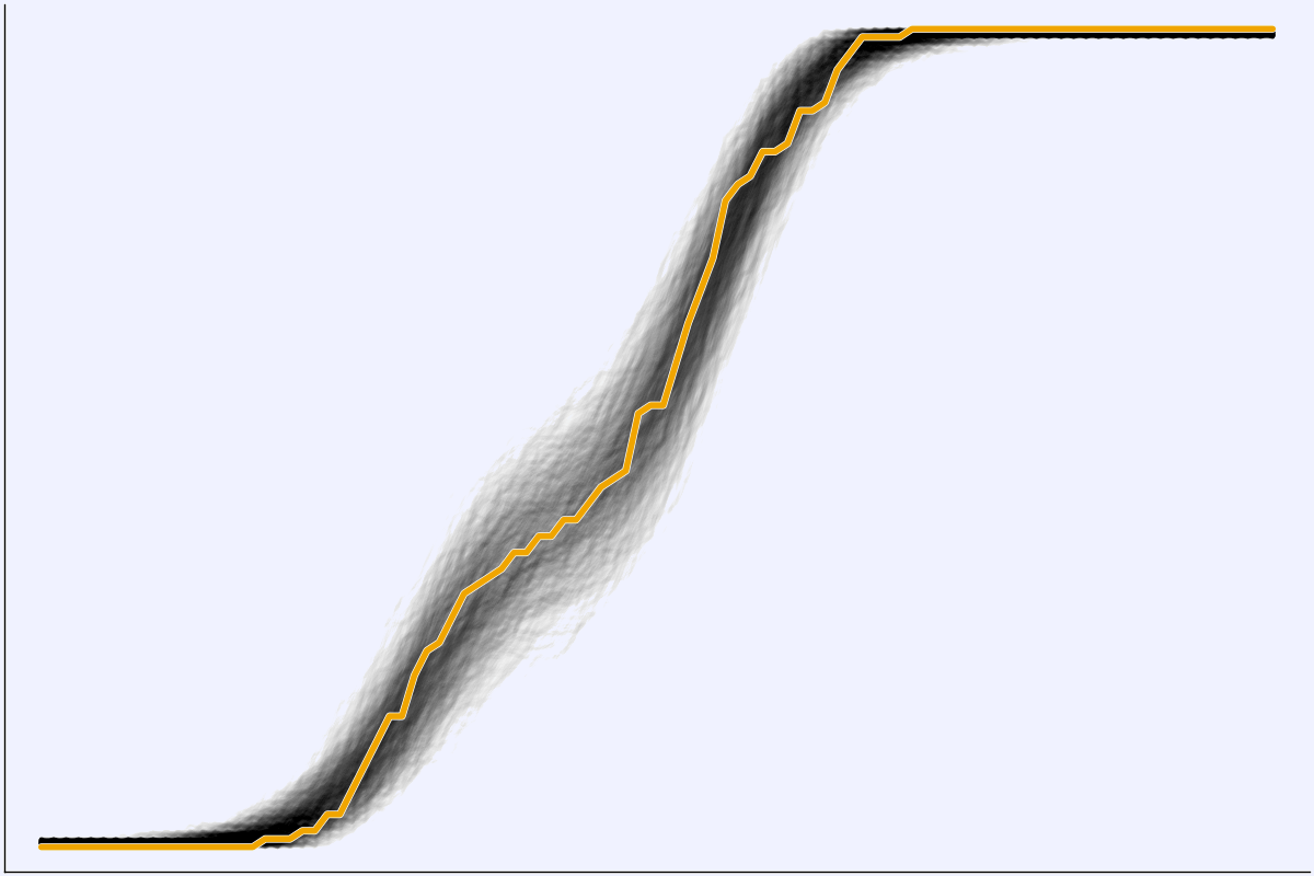
x
\theta_1
\theta_2
\theta_n
x^\text{rep}_1
x^\text{rep}_2
x^\text{rep}_2
\vdots
\vdots
x
Static Dependency Analysis
julia> lda
@model (α, η, K, V, N) begin
    M = length(N)
    β ~ Dirichlet(repeat([η],V)) |> iid(K)
    θ ~ Dirichlet(repeat([α],K)) |> iid(M)
    z ~ For(1:M) do m
            Categorical(θ[m]) |> iid(N[m])
        end
    w ~ For(1:M) do m
            For(1:N[m]) do n
                Categorical(β[(z[m])[n]])
            end
        end
end
julia> dependencies(lda)
[] => :α
[] => :η
[] => :K
[] => :V
[] => :N
[:N] => :M
[:η, :V, :K] => :β
[:α, :K, :M] => :θ
[:M, :θ, :N] => :z
[:M, :N, :β, :z] => :wBlei, Ng, & Jordan (2003). Latent Dirichlet Allocation. JMLR, 3(4–5), 993–1022.
In the Works
- First-class models
- Symbolic simplification via SymPy or REDUCE
- Constant-space streaming models (particle or Kalman filter)
- Reparameterizations ("noncentering", etc)
- Deep learning via Flux
- Variational inference a la Pyro
- Simulation-based modeling via Turing
logo by James Fairbanks, on Julia Discourse site
JuliaCon 2019
July 21-27
Baltimore, MD
Thank You!
2019-04-25 Global Artificial Intelligence Seattle
By Chad Scherrer


