Stochastic Bayesian model reduction for probabilistic machine learning

Dimitrije Marković


TNB meeting 21.03.2023

I

  • Bayesian deep learning
  • Structured shrinkage priors
  • Bayesian model reduction
  • Examples

II

  • Predictive and sparse coding
  • Variational auto-encoders
  • BMR for VAEs?
  • Active VAEs?
  • Bayesian deep learning
  • Structured shrinkage priors
  • Bayesian model reduction
  • Examples

Deep learning

\pmb{h}^n_0 = \pmb{x}^n \\ \vdots \\ \pmb{h}^n_i = \pmb{f}(\pmb{h}^n_{i-1}, \pmb{W}_{i}) \\ \vdots \\ \pmb{h}^n_L = \pmb{f}(\pmb{h}^n_{L-1}, \pmb{W}_{L}) \\ \pmb{y}^n \sim p(y|\pmb{W}, \pmb{x}^n) = p(y|\pmb{h}_L^n)
\pmb{W}^* = \argmin_{\pmb{W}} \sum_{n=1}^N \ln p(\pmb{y}^n|\pmb{W}, \pmb{x}^n)

Optimization


Bayesian deep learning

\pmb{h}^n_0 = \pmb{x}^n \\ \vdots \\ \pmb{h}^n_i = \pmb{f}(\pmb{h}^n_{i-1}, \pmb{W}_{i}) \\ \vdots \\ \pmb{h}^n_L = \pmb{f}(\pmb{h}^n_{L-1}, \pmb{W}_{L}) \\ \pmb{y}^n \sim p(y|\pmb{W}, \pmb{x}^n) = p(y|\pmb{h}_L^n)
p\left( \pmb{W} |\pmb{\mathcal{D}}\right)\propto p(\pmb{W}) \prod_{n=1}^N p(\pmb{y}^n|\pmb{W}, \pmb{x}^n)

Inference


Advantages

  • More robust, accurate and calibrated predictions
  • Learning from small datasets
  • Continuous learning (inference)
  • Distributed or federated learning (inference)
  • Marginalization
p\left(\pmb{Y}_{test}|\pmb{X}_{test} \right) = \int d \pmb{W} p\left(\pmb{Y}_{test}| \pmb{W}, \pmb{X}_{test} \right) p\left(\pmb{W}|\mathcal{D}_{train}\right)

Disadvantages

Solutions:

  • Mean-field approximation
  • Laplace approximation
  • Structured posterior

Extremely large number of parameters to express the posterior

p\left(\pmb{W}|\mathcal{D}_{train}\right)

How about using Bayesian model reduction?

  • Bayesian deep learning
  • Structured shrinkage priors
  • Bayesian model reduction
  • Examples

Bayesian deep learning

\pmb{h}^n_0 = \pmb{x}^n \\ \vdots \\ \pmb{h}^n_i = \pmb{f}(\pmb{h}^n_{i-1}, \pmb{W}_{i}) \\ \vdots \\ \pmb{h}^n_L = \pmb{f}(\pmb{h}^n_{L-1}, \pmb{W}_{L}) \\ \pmb{y}^n \sim p(y|\pmb{W}, \pmb{x}^n) = p(y|\pmb{h}_L^n)
p\left( \pmb{W} |\pmb{\mathcal{D}}\right)\propto p(\pmb{W}) \prod_{n=1}^N p(\pmb{y}^n|\pmb{W}, \pmb{x}^n)

Inference


Structured shrinkage priors

Nalisnick, Eric, José Miguel Hernández-Lobato, and Padhraic Smyth. "Dropout as a structured shrinkage prior." International Conference on Machine Learning. PMLR, 2019.

Ghosh, Soumya, Jiayu Yao, and Finale Doshi-Velez. "Structured variational learning of Bayesian neural networks with horseshoe priors." International Conference on Machine Learning. PMLR, 2018.

Dropout as a spike-and-slab prior

p(w_{lij}) \propto \lambda_{lij} \mathcal{N}(0, \sigma_0^2) + (1-\lambda_{lij}) \delta(w_{lij}) \\ \lambda_{lij} \sim \mathcal{Be}(\pi_l)

Better shrinkage priors 

p(w_{lij}) = \mathcal{N}(0, v_l^2 \tau_{li}^2 \lambda_{lij}^2) \\ \lambda_{lij} \sim p(\lambda|\tau_{li}), \: \tau_{li} \sim p(\tau|v_l), \: v_l \sim p(v)

Regularized horseshoe prior

Piironen, Juho, and Aki Vehtari. "Sparsity information and regularization in the horseshoe and other shrinkage priors." Electronic Journal of Statistics 11.2 (2017): 5018-5051.

c^2_l \sim \Gamma^{-1}(2, 3) \\ v_{l} \sim C^+(0, v_0) \\ \tau_{li} \sim C^+(0, v_l) \\ \lambda_{lij} \sim C^+(0, 1) \text{ if } l = 0 \text{ else } 1 \\ \gamma_{lij}^2 = \frac{c_l^2 \lambda_{lij}^2 \tau_{li} ^2}{c_l^2 + \lambda_{lij}^2 \tau_{li}^2}\\ w_{lij} \sim \mathcal{N} \left(0, \gamma_{lij}^2 \right)
\pmb{W} = (\pmb{W}_1, \ldots, \pmb{W}_L) \\ \pmb{W}_l = \left[ w_{lij} \right]_{1 \leq i \leq D_{l}, 1 \leq j \leq D_{l-1}}
  • Bayesian deep learning
  • Structured shrinkage priors
  • Bayesian model reduction
  • Examples

Bayesian model reduction

Two generative processes for the data

p\left( \pmb{z}|\mathcal{D} \right) \propto p\left( \mathcal{D}| \pmb{z}\right) p\left( \pmb{z} \right)

full model

\tilde{p}\left( \pmb{z}|\mathcal{D} \right) \propto p\left( \mathcal{D}| \pmb{z}\right) \tilde{p}\left( \pmb{z} \right)

reduced model 

-\ln \tilde{p}(\mathcal{D}) = - \ln p(\mathcal{D}) - \ln \int d \pmb{z} p(\pmb{z}|\mathcal{D}) \frac{\tilde{p}(\pmb{z})}{p(\pmb{z})}
-\ln \tilde{p}(\mathcal{D}) \approx F\left[ \pmb{\phi}^* \right] - \ln \int d \pmb{z} q\left(\pmb{z}| \pmb{\phi}^* \right) \frac{\tilde{p}(\pmb{z})}{p(\pmb{z})}

Karl Friston, Thomas Parr, and Peter Zeidman. "Bayesian model reduction." arXiv preprint arXiv:1805.07092 (2018).

Bayesian model reduction for BDL

Two generative processes for the data

p\left( \pmb{z}|\mathcal{D} \right) \propto p\left( \mathcal{D}| \pmb{z}\right) p\left( \pmb{z} \right)

full model

\tilde{p}\left( \pmb{z}|\mathcal{D} \right) \propto p\left( \mathcal{D}| \pmb{z}\right) \tilde{p}\left( \pmb{z} \right)

reduced model 

\tilde{p}_m(\pmb{z}) = \prod_{i \in P_m} \delta(z_i) \prod_{j \not\in P_m} \mathcal{N}(0, \sigma_0^2), \forall m \in \left \{1, \ldots, 2^D \right\}
m^* = \underset{m}{\text{argmax}} \ln \int d \pmb{z} q\left(\pmb{z} \right) \frac{\tilde{p}_m(\pmb{z})}{p(\pmb{z})}

Beckers, Jim, et al. "Principled Pruning of Bayesian Neural Networks through Variational Free Energy Minimization." arXiv preprint arXiv:2210.09134 (2022).

\ln \tilde{q}_{m^*}(\pmb{z}) = \ln q(\pmb{z}) + \ln \frac{\tilde{p}_m(\pmb{z})}{p(\pmb{z})} - \ln E_{q}\left[\frac{\tilde{p}_m(\pmb{z})}{p(\pmb{z})} \right]

BDL with shrinkage priors

p(\pmb{W}, \pmb{\gamma}|\pmb{\mathcal{D}})\propto p(\pmb{\gamma}) p(\pmb{W}|\pmb{\gamma}) \prod_{i=1}^N p(y_n|\pmb{W}, \pmb{x}_n)

Hierarchical model

p(\pmb{W}|\pmb{\gamma}) = \prod_i \prod_j \prod_l \mathcal{N}\left(w_{lij}; 0, \gamma_{lij}^2 \right)
p(\pmb{\gamma}) \rightarrow \text{Regularised horseshoe}

Factorization

q(\pmb{z}|\pmb{\phi}) = q(\pmb{z}_K)\prod_{i=1}^{K-1} q(\pmb{z}_i|\pmb{z}_{i+1})\quad (1) \\ q(\pmb{z}|\pmb{\phi}) = q(\pmb{z}_1)\prod_{i=2}^K q(\pmb{z}_i|\pmb{z}_{i-1})\quad (2) \\ q(\pmb{z}|\pmb{\phi}) = \prod_{i=1}^K q(\pmb{z}_i)\quad (3) \\

Approximate posterior

p(\pmb{z}|\pmb{\mathcal{D}})\propto p(\pmb{z}_K) p(\mathcal{D}|\pmb{z}_1) \prod_{i=1}^{K-1} p(\pmb{z}_i|\pmb{z}_{i+1})

Hierarchical model

Non-centered parameterization

Approximate posterior

p(\pmb{\tilde{z}}|\pmb{\mathcal{D}})\propto p(\mathcal{D}|\pmb{\tilde{z}}_1, \ldots, \pmb{\tilde{z}}_K) \prod_{i=1}^{K} p(\pmb{\tilde{z}}_i)

Hierarchical model

q\left(\pmb{\tilde{z}}|\pmb{\tilde{\phi}}\right) = \prod_{i=1}^K q(\pmb{\tilde{z}}_i|\tilde{\pmb{\phi}}_i)
F = \sum_{i=1}^K F[\pmb{\tilde{\phi}}_i] \\ F\left[ \pmb{\tilde{\phi}}_i\right] = E_{q(\pmb{\tilde{z}}_i)}\left[ f(\pmb{\tilde{z}}_i) + \ln q(\pmb{\tilde{z}}_i) \right]\\ f(\pmb{\tilde{z}}_i) = - \frac{1}{K} \int q(\pmb{\tilde{z}}_{\backslash i}) \ln \left[ p(\pmb{\tilde{z}}_i)^Kp(D|\pmb{\tilde{z}}) \right] \prod_{j\neq i} d \pmb{\tilde{z}}_j

Variational free energy

Stochastic variational inference

Stochastic gradient

F = \sum_i F\left[ \pmb{\tilde{\phi}}_i\right] \rightarrow \dot{\pmb{\tilde{\phi}}}_i = - \nabla_{\pmb{\tilde{\phi}}_i} F\left[ \pmb{\tilde{\phi}}_i\right]
\hat{f}(\pmb{\tilde{z}}_i) = - \frac{1}{S\cdot K}\sum_{s} \ln \left[ p(\pmb{\tilde{z}}_i)^K p(D^n|\pmb{\tilde{z}}^s, \pmb{\tilde{z}}_i) \right]
\mathcal{D}^n \sub D, \qquad \pmb{\tilde{z}}^s \sim q(\pmb{\tilde{z}})
\nabla_{\pmb{\tilde{\phi}}_i} \hat{F}\left[ \pmb{\tilde{\phi}}_i\right] = \frac{1}{S} \sum_s \nabla_{\pmb{\tilde{\phi}}_i} \ln q(\pmb{\tilde{z}}_i^s) \left[\hat{f}(\pmb{\tilde{z}}_i^s) + \ln q(\pmb{\tilde{z}}_i^s) \right]
\nabla_{\pmb{\tilde{\phi}}_i} F\left[ \pmb{\tilde{\phi}}_i\right] = E_{q(\pmb{\tilde{z}}_i)}\left[ \nabla_{\pmb{\tilde{\phi}}_i} \ln q(\pmb{\tilde{z}}_i) \left( f(\pmb{\tilde{z}}_i) + \ln q(\pmb{\tilde{z}}_i) \right) \right]\\

Stochastic BMR for BDL

p\left( \pmb{W}|\mathcal{D} \right) \propto p\left( \mathcal{D}| \pmb{W} \right) p\left( \pmb{W} \right)

flat model

p\left( \pmb{W}|\mathcal{D}, \pmb{\gamma} \right) p\left ( \pmb{\gamma} | \pmb{D} \right) \propto p\left( \mathcal{D}| \pmb{W} \right) p\left( \pmb{W}|\pmb{\gamma} \right) p(\pmb{\gamma})

extended model

F = \int d \pmb{\gamma} q(\pmb{\gamma}) \ln \frac{q(\pmb{\gamma})}{p(\mathcal{D}|\pmb{\gamma})p(\pmb{\gamma})}
\approx \int d \pmb{\gamma} q(\pmb{\gamma}) \left[ - \ln E_{q^*(\pmb{W})}\left[ \frac{p(\pmb{W}|\pmb{\gamma})}{p(\pmb{W})} \right] + \ln \frac{q(\pmb{\gamma})}{p(\pmb{\gamma})}\right] \equiv \tilde{F}
-\ln p(\mathcal{D}|\pmb{\gamma}) \approx F^* - \ln E_{q^*(\pmb{W})} \left[ \frac{p(\pmb{W}|\pmb{\gamma})}{p(\pmb{W})} \right]

BMR algorithm

p\left( \pmb{W}|\mathcal{D} \right) \propto p\left( \mathcal{D}| \pmb{W} \right) p\left( \pmb{W} \right)
p\left( \pmb{W}|\mathcal{D}, \pmb{\gamma} \right) \approx q\left( \pmb{W}| \pmb{\gamma} \right)
\ln q(\pmb{W}|\pmb{\gamma}) = \ln q(\pmb{W}|\pmb{\phi}^*) + \ln \frac{p(\pmb{W}|\pmb{\gamma})}{p(\pmb{W})} - \ln E_{q^*}\left[\frac{p(\pmb{W}|\pmb{\gamma})}{p(\pmb{W})} \right]
\dot{\pmb{\phi}} = - \nabla \hat{F}[\pmb{\phi}]

Step 1

BMR algorithm

p\left( \pmb{\gamma}|\mathcal{D} \right) \propto p\left( \mathcal{D}| \pmb{\gamma} \right) p\left( \pmb{\gamma} \right)
\bar{q}(\pmb{W}) = \int d\pmb{W} q(\pmb{W}|\pmb{\gamma}) q(\pmb{\gamma}) \approx \prod_l \prod_i \prod_j \mathcal{N}\left(\bar{\pmb{\mu}}_{lij}, \bar{\pmb{\sigma}}^2_{lij} \right)
\dot{\pmb{\lambda}} = \nabla_{\pmb{\lambda}} \tilde{F}[\pmb{\lambda}], \:\: p\left( \pmb{\gamma}|\mathcal{D} \right) \approx q(\pmb{\gamma}|\pmb{\lambda})

Step 2

New epoch

\( p(\pmb{W}) \propto \int d \pmb{\gamma}   p_{W|\gamma}q_{\gamma}  \)

step 1

\(\vdots\)

step 2

w_{lij} = 0, \text{ if } \frac{\bar{\pmb{\mu}}_{lij}}{\bar{\pmb{\sigma}}_{lij}} < c

Pruning

  • Bayesian deep learning
  • Structured shrinkage priors
  • Bayesian model reduction
  • Examples
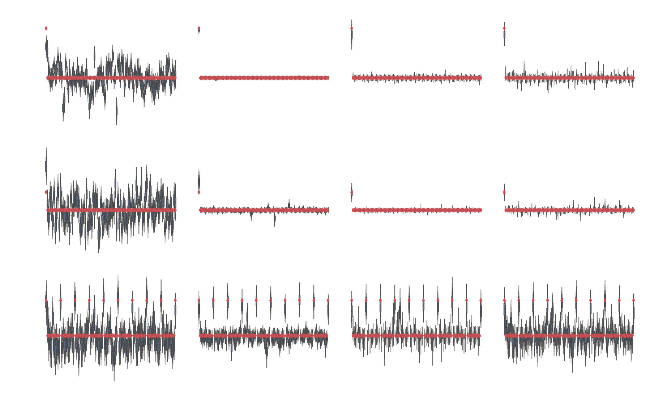
\pmb{x}_n \sim \mathcal{N}_D \left(0, \pmb{I} \right) \\ y_n \sim p\left( y| \pmb{W} \cdot \pmb{x}_n \right) \\ w_1 = 1, w_{d>1} = 0

Regression

Linear (D=(1,100), N=100)

\mathcal{N}\left(y; \pmb{W} \cdot \pmb{x}_n, \sigma^2 \right)

Logistic (D=(1,100), N=200)

\mathcal{Be}\left(y|s(\pmb{W} \cdot \pmb{x}_n)\right)

Multinomial (D=(10,10), N=300)

\mathcal{Cat}\left(y|\rho(\pmb{W} \cdot \pmb{x}_n)\right)

Regression comparison

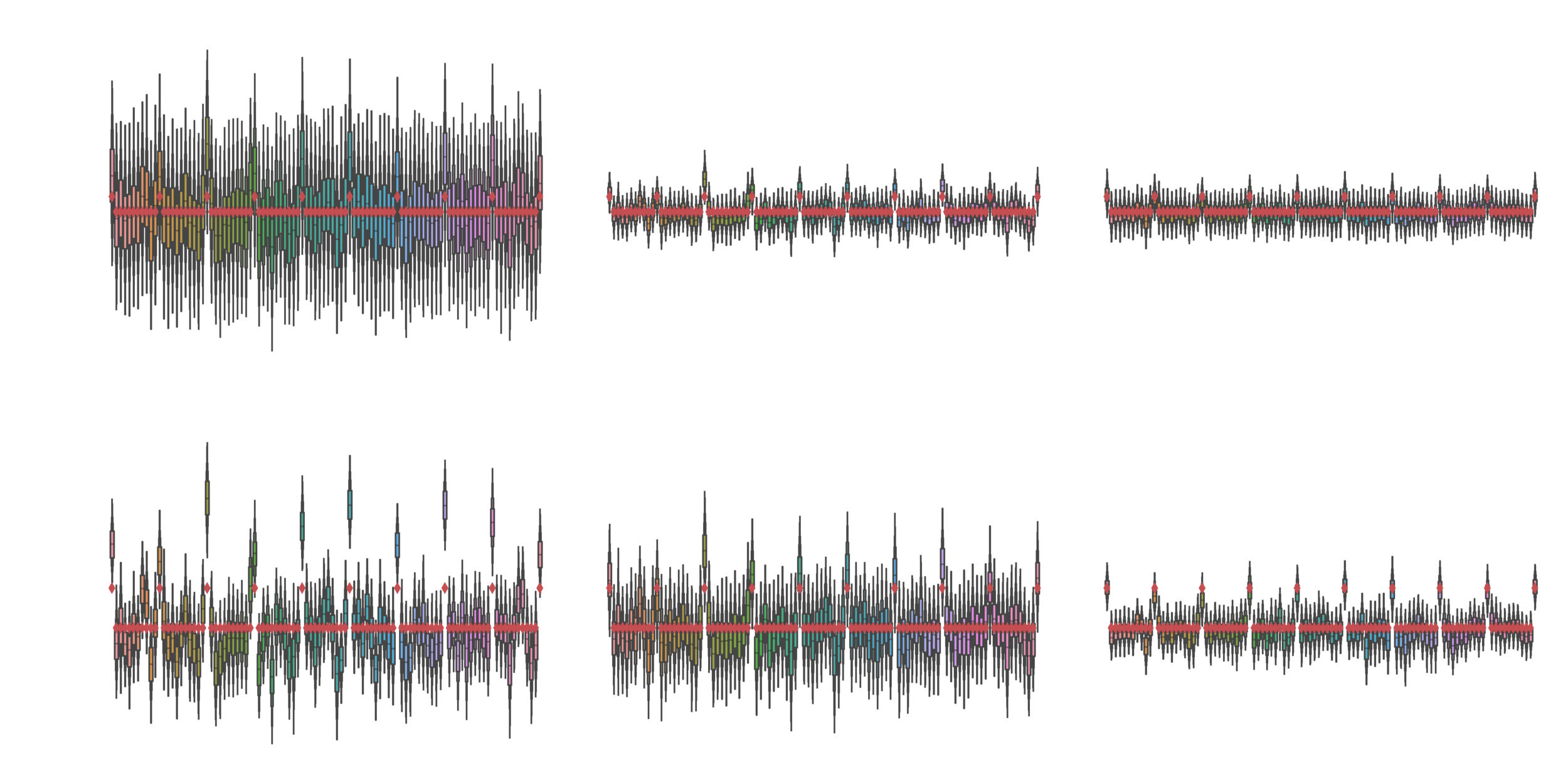
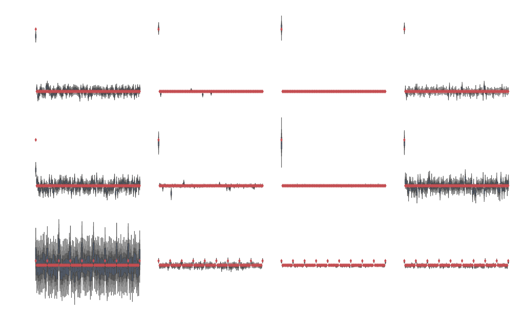
Nonlinear problem

D_{in} = 100, \: f(\pmb{x}_n, \pmb{W}) = ReLU(x_{n, 1}), \: y_n \sim \mathcal{N}(f(\pmb{x}_n, \pmb{W}), 1)

Normal likelihood

N = 2000, \quad \pmb{x}_n \sim \mathcal{N}_{D_{in}} \left(0, \pmb{I} \right)
D_{in} = 100, \: f(\pmb{x}_n, \pmb{W}) = ReLU(x_{n, 1}), \: y_n \sim \mathcal{Be}\left(s(f(\pmb{x}_n, \pmb{W})\right)

Bernoulli likelihood

D_{in} = 19, D_{out} = 10 \\ f_c(\pmb{x}_n, \pmb{W}) = ReLU(x_{n, c}), \forall c \in \{1, \ldots, D_{out}\} \\ y_n \sim \mathcal{Cat}\left(\pmb{\rho}\right), \: \rho_c \propto e^{f_c}

Categorical likelihood

Neural network model

D_{in} = 100, D_{h} = 20, D_{out}=1 \\ f(\pmb{x}_n, \pmb{W}) = W_2 \cdot ReLU(\pmb{W}_1 \cdot \pmb{x}_{n})

Normal and Bernoulli likelihoods

D_{in} = 10, D_h = 101, D_{out} = 10 \\ f(\pmb{x}_n, \pmb{W}) = W_2 \cdot ReLU(\pmb{W}_1 \cdot \pmb{x}_{n})

Categorical likelihood

\pmb{\beta} = \pmb{W}_2 \cdot \pmb{W}_1

Iterative improvements

Comparison

Leave one out cross validation
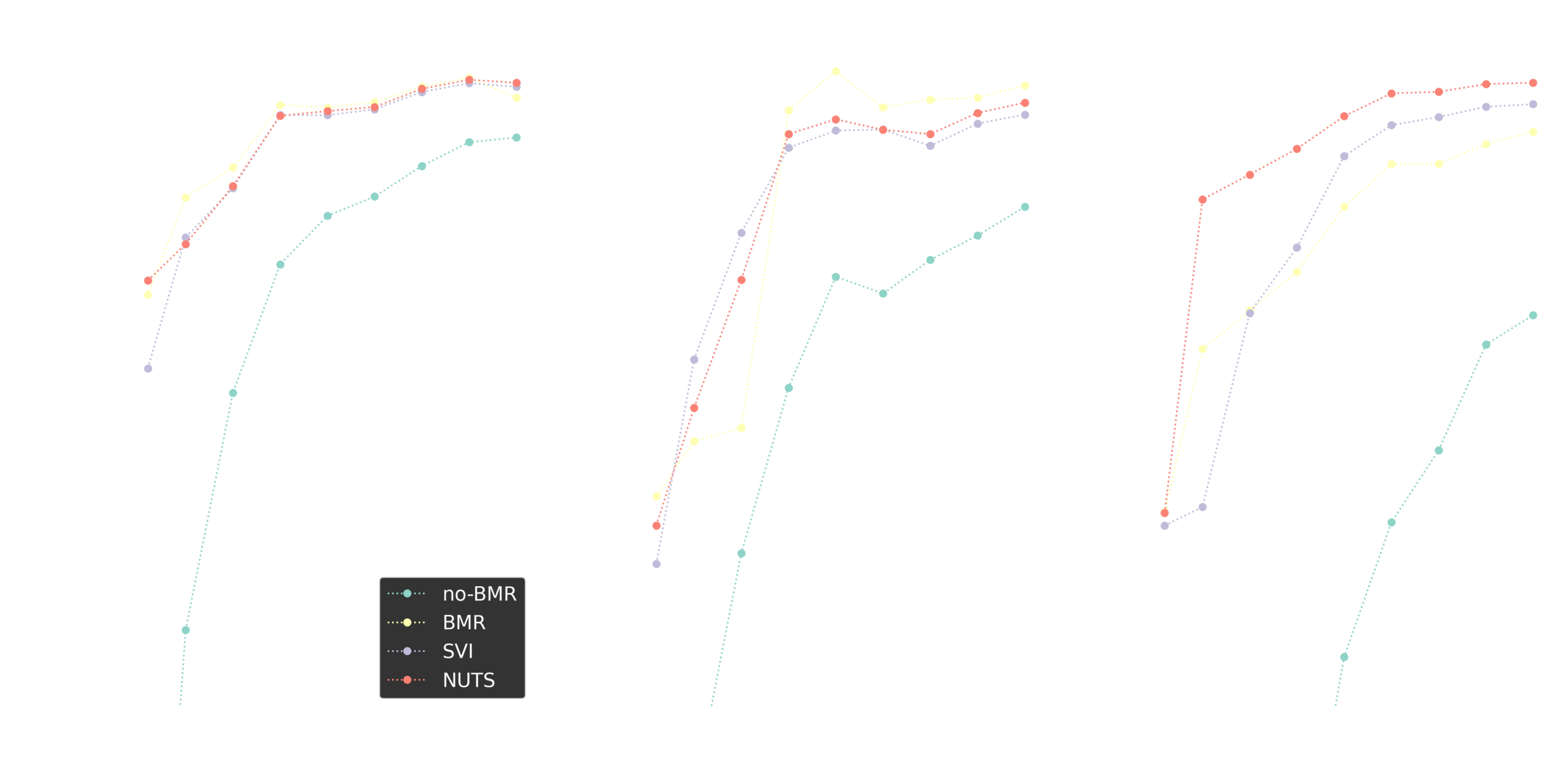
Image classification

Fashion MNIST
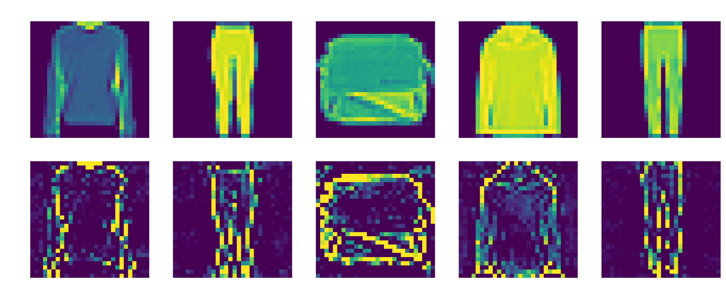
Image classification
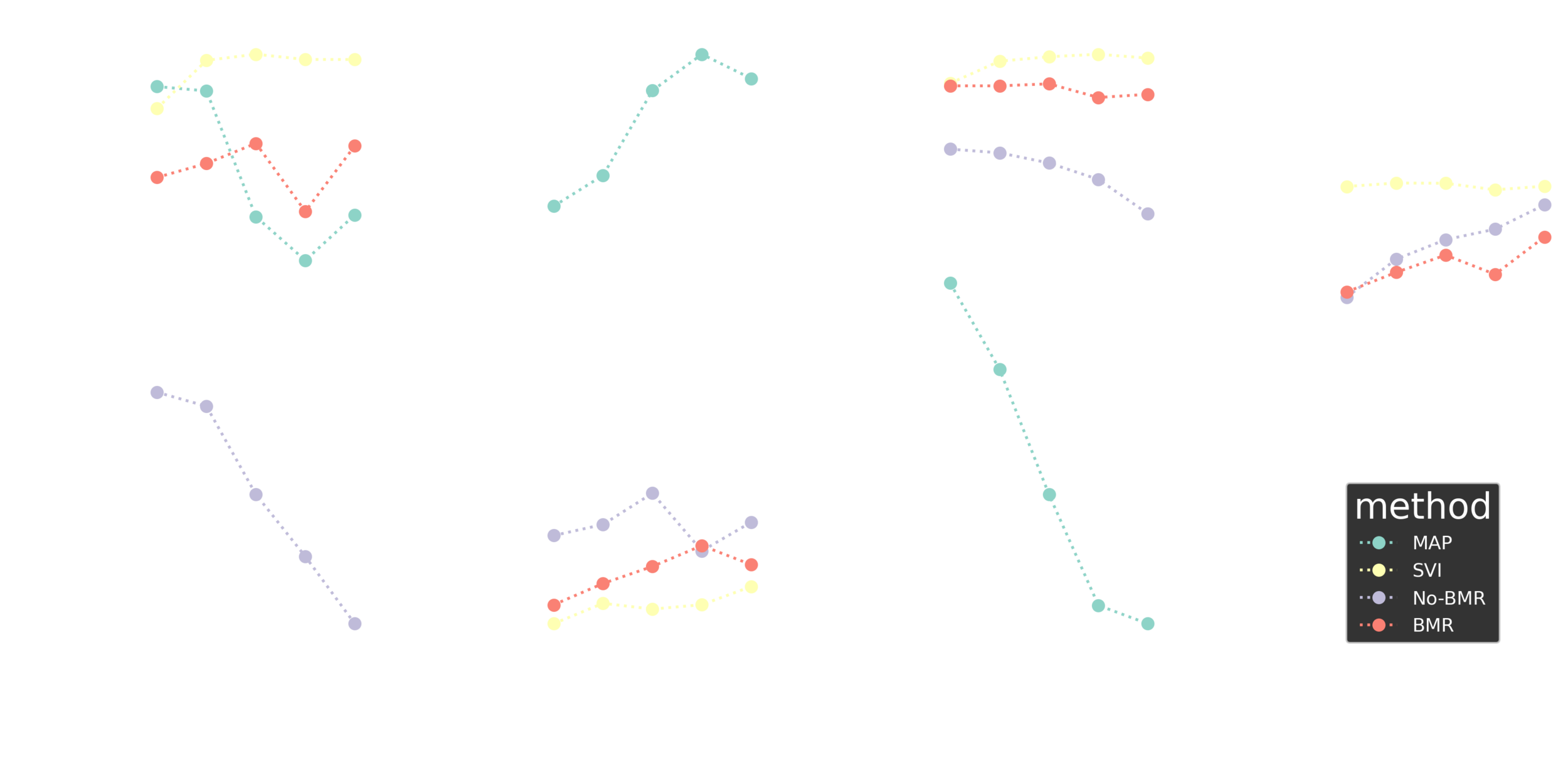
Summary I

Stochastic BMR seems to work great and shows a potential for a range of deep learning applications.

https://github.com/dimarkov/numpc

Idea: might be possible to prune large pre-trained models using Laplace approximation.

We could probably use SBMR in generative models such as Variatonal autoencoders.

Naturally complements distributed and federated inference problems.

The second part

Beyond BDL

Probabilistic ML for edge devices

Bring ML/AI algorithms to a hardware with a range of compute capabilities. 

Privacy preserving distributed computing.

Computationally efficient and biologically inspired learning and inference.

Contemplations on how to combine active inference, predictive coding, sparse coding, variational auto-encoders and bayesian model reduction?

II

  • Predictive coding
  • Variational auto-encoders
  • Sparse coding
  • BMR for VAEs?
  • Active VAEs?

II

  • Predictive coding
  • Variational auto-encoders
  • Sparse coding
  • BMR for VAEs?
  • Active VAEs?

Predictive coding

PC postulates that the brain is constantly adapting a generative model of the environment:

  • top - down -> predictions of sensory signals
  • bottom - up -> prediction errors 

Millidge, Beren, Anil Seth, and Christopher L. Buckley. "Predictive coding: a theoretical and experimental review." arXiv preprint arXiv:2107.12979 (2021).

Paradigms:

  • Unsupervised predictive coding
  • Supervised predictive coding:
    • Generative or discriminative 

Supervised PC

Song, Yuhang, et al. "Can the brain do backpropagation?---exact implementation of backpropagation in predictive coding networks." Advances in neural information processing systems 33 (2020): 22566-22579.

Generative

Discriminative

\(y\)

\(z\)

\(X\)

\(X\)

\(z\)

\(y\)

\pmb{z}^n_0 = \pmb{X}^n \\ \vdots \\ \pmb{z}^n_i = \pmb{f}(\pmb{z}^n_{i-1}, \pmb{W}_{i}) + \epsilon^n_i \\ \vdots \\ \pmb{z}^n_L = \pmb{f}(\pmb{z}^n_{L-1}, \pmb{W}_{L}) + \epsilon^n_L \\ \pmb{y}^n = \pmb{g}(\pmb{z}^n_L, \pmb{W}_y) + \epsilon^n_y

Supervised PC

Song, Yuhang, et al. "Can the brain do backpropagation?---exact implementation of backpropagation in predictive coding networks." Advances in neural information processing systems 33 (2020): 22566-22579.

Equivalence between backpropagation based training of ANNs and inference and learning based training of SPCNs

Distributed inference, and layer specific Hebbian like learning of weights.

MAP estimates of latent states, and MLE estimate of weights. 

Unsupervised PC

\(y\)

\(z\)

\(X\)

A proper generative model of various sensory modalities.

Both generative and discriminative.

Link to variational auto-encoders.

II

  • Predictive coding
  • Variational auto-encoders
  • Sparse coding
  • BMR for VAEs?
  • Active VAEs?

Variational auto-encoders

\(z\)

\( \pmb{\mathcal{D}} \)

\( \pmb{\mathcal{D}} \)

Encoder

Decoder

\( p(\pmb{\mathcal{D}}| \pmb{z}) \)

\( q( \pmb{z}|\pmb{\mathcal{D}}) \)

Unlike PC, VAE use amortized variational inference - for its efficiency and scalability

Biological connection

Marino, Joseph. "Predictive coding, variational autoencoders, and biological connections." Neural Computation 34.1 (2022): 1-44.

q(\pmb{z}) = \mathcal{N}\left( \pmb{\mu}_z, \pmb{\Sigma}_z \right), \:\: \pmb{\lambda} = \left[ \pmb{\mu}_z, \pmb{\Sigma}_z \right] \\ q(\pmb{\theta}) = \mathcal{N}\left( \pmb{\mu}_{\theta}, \pmb{\Sigma}_{\theta} \right), \:\: \pmb{\phi} = \left[ \pmb{\mu}_{\theta}, \pmb{\Sigma}_\theta \right]
F = \int q(\pmb{z}) \ln \frac{q(\pmb{z})}{p(\pmb{z}|\pmb{\theta})p(\pmb{\mathcal{D}}|\pmb{z}, \pmb{\theta})} + \int q(\pmb{\theta}) \ln \frac{q(\pmb{\theta})}{p(\pmb{\theta})}
\dot{ \pmb{\lambda}} = - \nabla_{\pmb{\lambda}} F, \:\: \dot{ \pmb{\phi}} = - \nabla_{\pmb{\phi}} F

Bayesian inference and learning for PCNs

Biological connection

Marino, Joseph. "Predictive coding, variational autoencoders, and biological connections." Neural Computation 34.1 (2022): 1-44.

F = \int q(\pmb{z}|\pmb{\mathcal{D}}) \ln \frac{q(\pmb{z}|\pmb{\mathcal{D}})}{p(\pmb{z}|\pmb{\theta})p(\pmb{\mathcal{D}}|\pmb{z}, \pmb{\theta})} + \int q(\pmb{\theta}) \ln \frac{q(\pmb{\theta})}{p(\pmb{\theta})}
\pmb{\lambda} \leftarrow \pmb{f}_{\pmb{\gamma}}\left(\pmb{\mathcal{D}} \right)

Bayesian inference and learning for VAEs

Amortized inference

Iterative amortized inference

\pmb{\lambda} \leftarrow \pmb{f}_{\gamma}\left(\pmb{\lambda}, \nabla_{\lambda} F \right)

II

  • Predictive coding
  • Variational auto-encoders
  • Sparse coding
  • BMR for VAEs?
  • Active VAEs?

Sparse coding

SC postulates that sensory stimuli is encoded by the strong activation of a relatively small set of neurons.

Efficient representation: e.g. sparse coding of natural images leads to wavelet-like (gabor) filters filters that resemble the receptive fields of simple cells in the visual cortex

SC postulates that sensory stimuli is encoded by the strong activation of a relatively small set of neurons.

Principle assumption in spiking neuronal networks.

Numerous applications in ML and an inspiration for sparse variational autoencoders.

Illing, Bernd, Wulfram Gerstner, and Johanni Brea. "Biologically plausible deep learning—but how far can we go with shallow networks?." Neural Networks 118 (2019): 90-101.

Sparse coding math

Boutin, Victor, et al. "Sparse deep predictive coding captures contour integration capabilities of the early visual system." PLoS computational biology 17.1 (2021): e1008629.

\pmb{z}_{L-1} = W_L^T \pmb{z}_L + \pmb{\epsilon}_L; \:\: || \pmb{z}_L||_p \leq \alpha_L; \:\: z_{L, i} \geq 0 \\ \vdots \\ \pmb{z}_{1} = W_2^T \pmb{z}_2 + \pmb{\epsilon}_2; \:\: || \pmb{z}_2||_p \leq \alpha_2; \:\: z_{2, i} \geq 0 \\ \pmb{x} = W_1^T \pmb{z}_1 + \pmb{\epsilon}_1; \:\: || \pmb{z}_1||_p \leq \alpha_1; \:\: z_{1, i} \geq 0

Sparse coding math

Boutin, Victor, et al. "Sparse deep predictive coding captures contour integration capabilities of the early visual system." PLoS computational biology 17.1 (2021): e1008629.

\pmb{z}^*_1, \ldots, \pmb{z}^*_L = \underset{\pmb{z}_1, \ldots, \pmb{z}_L > 0}{\mathrm{min}} \frac{1}{2} \sum_l \kappa_l \left( \underbrace{\pmb{z}_{l} - W_{l+1}^T \pmb{z}_{l+1}}_{\epsilon_l}\right)^2 + 2 \gamma_l ||\pmb{z_l}||_p
\dot{\pmb{u}}_l = - \pmb{u}_l + \kappa_l \pmb{W}_l \epsilon_l - \kappa_{l+1} \epsilon_{l+1} + \pmb{z}_l
\dot{\pmb{u}}_l = - \pmb{u}_l + \kappa_l \pmb{W}_l \pmb{z}_{l-1} + \kappa_{l+1} \pmb{W}_{l+1}^T \pmb{z}_{l+1} - \pmb{V}_l \pmb{z}_l \\ V_l = \pmb{W}_l \pmb{W}_{l+1}^T + (\kappa_l + \kappa_{l+1} - 2) \pmb{I} \\ \pmb{z}_l = f_p(\pmb{u}_l, \gamma_l); \:\: \pmb{u_l} = f^{-1}_p(\pmb{z}_l, \gamma_l) = \pmb{z}_l - \gamma_l \partial_{\pmb{z}_l} ||\pmb{z}_l||_p

Sparse variational autoencoders

Asperti, Andrea. "Sparsity in variational autoencoders." arXiv preprint arXiv:1812.07238 (2018).

Barello, Gabriel, Adam S. Charles, and Jonathan W. Pillow. "Sparse-coding variational auto-encoders." BioRxiv (2018): 399246.

Kandemir, Melih. "Variational closed-form deep neural net inference." Pattern Recognition Letters 112 (2018): 145-151.

Incorporate sparse coding assumptions into variational auto-encoders for a  proper probabilistic treatment. 

Does structural sparsity result in activation sparsity?

Dynamical sparse coding

\pmb{z}_{L-1}^{t+1} = W_L^T \pmb{z}_L^t + A_L^T \pmb{z}_{L-1}^t + \pmb{\epsilon}_L^{t+1}; \:\: || \pmb{z}_L^t||_p \leq \alpha_L; \:\: z_{L, i}^t \geq 0 \\ \vdots \\ \pmb{z}_{1}^{t+1} = W_2^T \pmb{z}_2^t + A_2^t \pmb{z}_1^t + \pmb{\epsilon}_2^{t+1}; \:\: || \pmb{z}_2^t||_p \leq \alpha_2; \:\: z_{2, i}^t \geq 0 \\ \pmb{x}_{t+1} = W_1^T \pmb{z}_1^t + A_1^T \pmb{x}_t + \pmb{\epsilon}_1^{t+1}; \:\: || \pmb{z}_1^t||_p \leq \alpha_1; \:\: z_{1, i}^t \geq 0

Generalised coordinates?

Dynamical sparsity?

Contextual dynamics

\(y_{t-1}\)

\(z\)

\(z_t\)

\(z\)

\(z_{t-1}\)

\(z\)

\(s_{t-1}\)

\(y_t\)

\(z\)

\(z_t\)

\(z\)

\(z_t\)

\(z\)

\(s_t\)

\(y_{t+1}\)

\(z\)

\(z_t\)

\(z\)

\(z_{t+1}\)

\(z\)

\(s_{t+1}\)

Switching linear dynamics?

II

  • Predictive coding
  • Variational auto-encoders
  • Sparse coding
  • BMR for VAEs?
  • Active VAEs?

BMR

Sparsification of variational auto-encoders

Structure learning (e.g. latent state graph topology)

F = \int q(\pmb{z}|\pmb{\mathcal{D}}) \ln \frac{q(\pmb{z}|\pmb{\mathcal{D}})}{p(\pmb{z}|\pmb{\theta})p(\pmb{\mathcal{D}}|\pmb{z}, \pmb{\theta})} + \int q(\pmb{\theta}) \ln \frac{q(\pmb{\theta})}{p(\pmb{\theta})}

II

  • Predictive coding
  • Variational auto-encoders
  • Sparse coding
  • BMR for VAEs?
  • Active VAEs?

Active inference

Active variational auto-encoders:

  • actively selecting salient parts of stimuli (data)
  • selecting most informative subset for training

Parr, Thomas, and Karl J. Friston. "Active inference and the anatomy of oculomotion." Neuropsychologia 111 (2018): 334-343.

Parr, Thomas, and Karl J. Friston. "The active construction of the visual world." Neuropsychologia 104 (2017): 92-101.

Parr, Thomas, and Karl J. Friston. "Working memory, attention, and salience in active inference." Scientific reports 7.1 (2017): 14678.

Active inference

  • Multi-agent systems:
    • emergent global generative models from interaction of simple agents implementing sparse active variational autoencoders. 
    • Active federated (distributed) inference and learning

Heins, Conor, et al. "Spin glass systems as collective active inference." arXiv preprint arXiv:2207.06970 (2022).

Friston, Karl J., et al. "Designing Ecosystems of Intelligence from First Principles." arXiv preprint arXiv:2212.01354 (2022).

Ahmed, Lulwa, et al. "Active learning based federated learning for waste and natural disaster image classification." IEEE Access 8 (2020): 208518-208531.

Summary II

Predictive and sparse coding <=> Variational auto-encoders

Challenges:

  • Defining Bayesian sparse predictive coding for time series data.
  • Using stochastic BMR for sparse structure learning.
  • Incorporating dynamic sparse VAEs into active inference agents.


Few references

Murphy, Kevin P. Probabilistic machine learning: an introduction. MIT press, 2022.

Wilson, Andrew Gordon. "The case for Bayesian deep learning." arXiv preprint arXiv:2001.10995 (2020).

Bui, Thang D., et al. "Partitioned variational inference: A unified framework encompassing federated and continual learning." arXiv preprint arXiv:1811.11206 (2018).

Murphy, Kevin P. Probabilistic machine learning: Advanced Topics. MIT Press 2023

Stochastic Bayesian model reduction for probabilistic machine learning

By dimarkov

Stochastic Bayesian model reduction for probabilistic machine learning

  • 49