Using Machine Learning for IPM profile reconstruction
D. Vilsmeier, M. Sapinski and R. Singh
(d.vilsmeier@gsi.de)
Can we use Machine Learning for IPM profile reconstruction?
- What is Machine Learning?
- What is space-charge induced profile distortion?
- How can we simulate this process?
- What machine learning techniques can be applied?
- How can we verify the simulation?
- What's next?
What is Machine Learning?
Field of study that gives computers the ability to learn without being explicitly programmed.
- Arthur Samuel (1959)


"Classical"
approach:
+
=
Input
Algorithm
Output
Machine
Learning:
+
=
Input
Algorithm
Output
What is Machine Learning really?
A computer program is said to learn from experience E with respect to some class of tasks T and performance measure P, if its performance at tasks in T, as measured by P, improves with experience E.
- Tom Mitchell (1997)
+
=
Input
Algorithm
Output
Input
+
Output
Experience
Performance
Task
A Brief History of AI
Arthur Samuel
Checkers
1959
Minsky, Papert
Perceptron limits
1969
Hans Moravec
Autonomously driving car
1979
1992
TD-Gammon
Gerald Tesauro
1997
Deep Blue
IBM
2015
Playing Atari Games
DeepMind
2017
AlphaZero
DeepMind
Machine Learning Toolbox
Supervised Learning:
- Artificial Neural Networks
- Decision Trees
- Linear Regression
- k-Nearest Neighbor
- Support Vector Machines
- Random Forest
- ... and many more
Unsupervised Learning:
- k-Means Clustering
- Autoencoders
- Principal comp. analysis
Reinforcement Learning:
- Q-Learning
- Deep Deterministic Policy Gradient
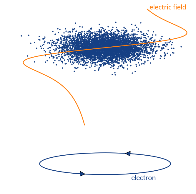
Ionization Profile Monitors
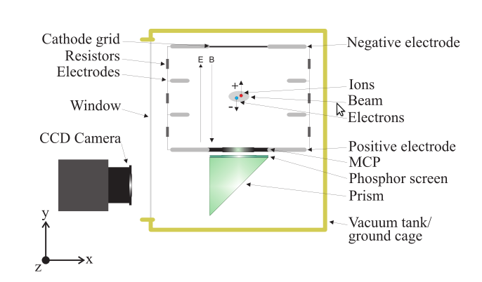
- Measure the transverse profile of particle beams
- Beam ionizes the rest gas
🡒 measure the ionization products
- Electric guiding field is used to transport ions / electrons to the detector
- For electrons optionally apply a magnetic field to confine trajectories
The Problem
Extracting the ions / electrons from the ionization region is expected to provide a one-dimensional projection of the transverse beam profile, but ...
| Protons | |
| Energy | 6.5 TeV |
| ppb | 2.1e11 |
| σ_x | 0.27 mm |
| σ_y | 0.36 mm |
| 4σ_z | 0.9 ns |
What happens?
Ideal case:
Particles move on straight lines towards the detector
Real case:
Trajectories are distorted due to various effects

IPM Profile Distortion
Initial momenta:
-
Initial velocity obtained in the ionization process may have a component along the profile
- Becomes significant for small extraction fields / small beam sizes
Interaction with beam fields:
-
Close to the beam particles interact with the beam fields, resulting in distorted trajectories
- Becomes significant for large beam fields, e.g. high charge densities or beam energies
+ instrumental effects such as camera tilt, point-spread-functions from optical system and multi-channel-plate granularity, etc.
Countermeasures

Increase electric guiding field
E_3 > E_2 > E_1
Increased electric field 🡒 smaller extraction times 🡒 smaller displacement
Additional magnetic guiding field
Increased magnetic field 🡒 smaller gyroradius 🡒 smaller possible displacement
B_1 \;\;\; < \;\;\; B_2
Space-charge interaction
6.5 TeV, 2.1e11 Protons, σ = (270, 360) μm, 4σz = 0.9ns
- Interaction with beam fields can become very strong 🡒 extraction fields are not sufficient to suppress distortion (typical values are 50 kV/m)
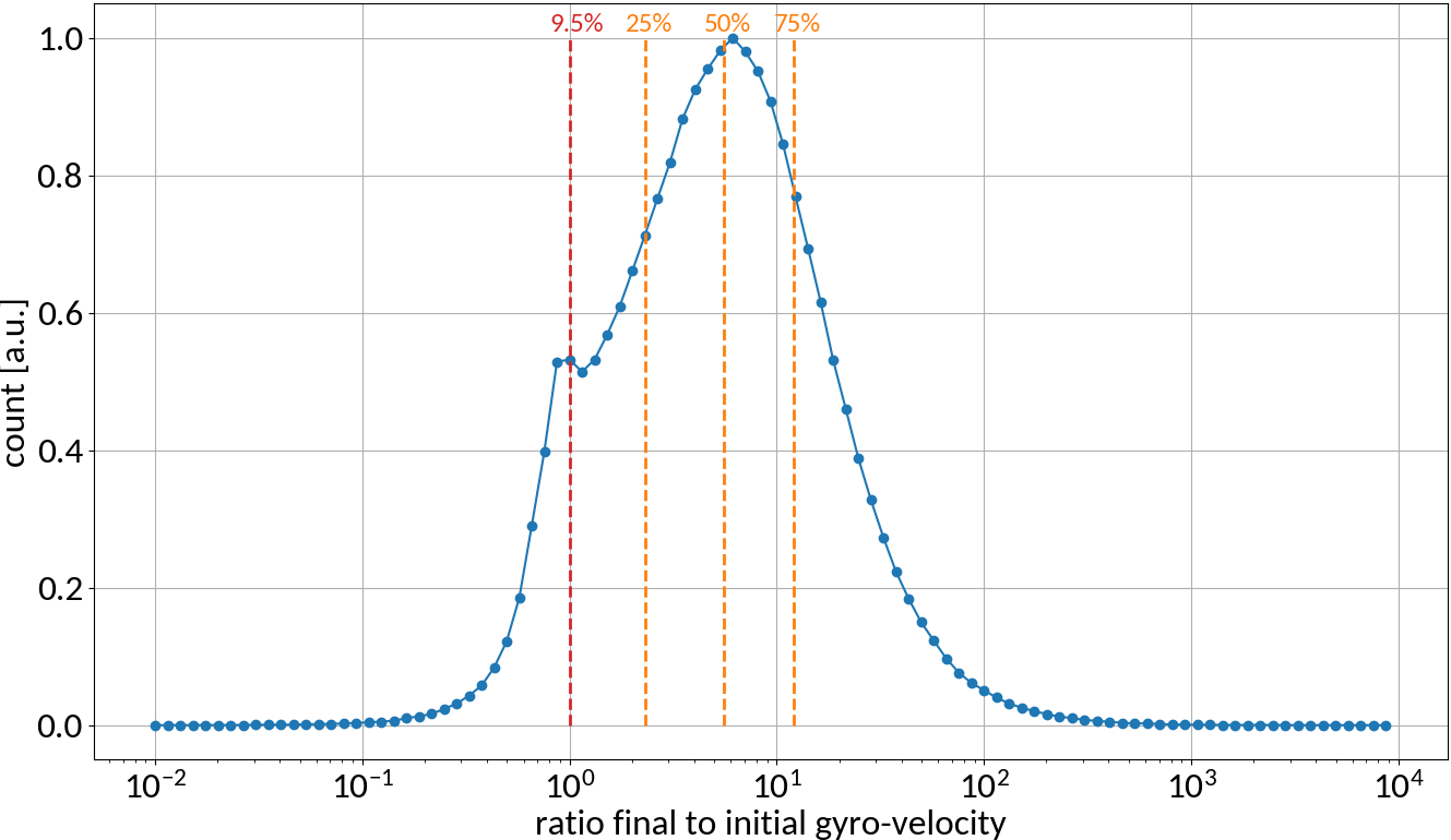
- Space-charge interaction results in a vast increase of gyro-velocities and hence in large displacements
Space-charge interaction
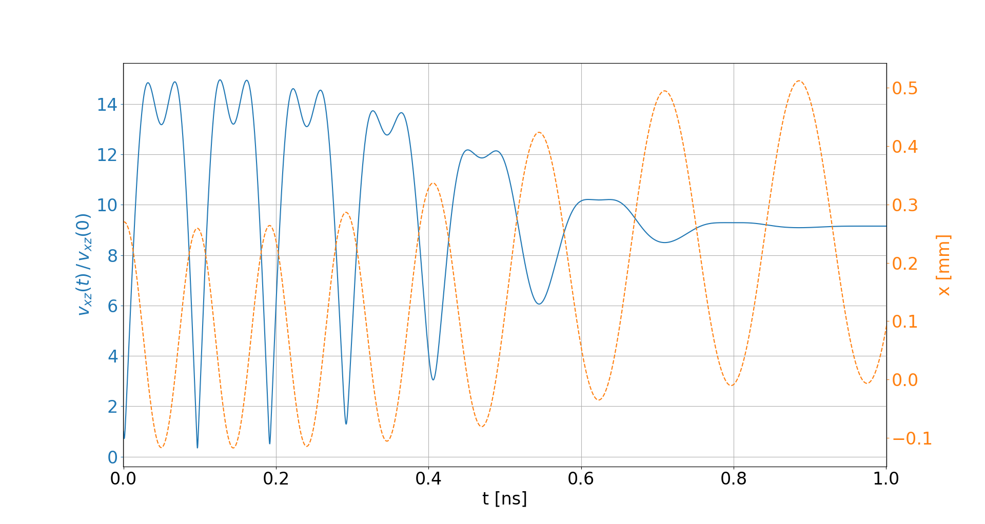
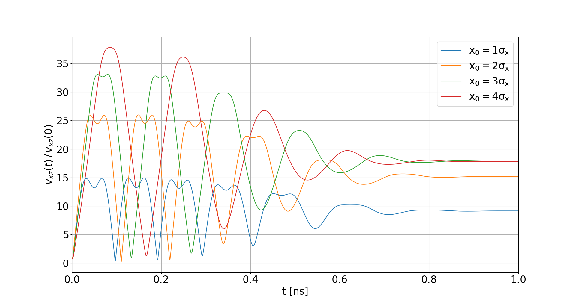
-
Electron velocities oscillate in the electric field of the beam
- They level off at an increased velocity, hence increasing distortion
- The amplitude of this oscillation depends on the initial offset to the beam center
Analytical considerations
Actually this type of oscillation can be seen from analytical considerations, using a simplified, namely linear, model for the beam electric field. This assumption holds well for the region close to the beam center.
The corresponding equations of motion are (for an electron):
\ddot{\vec{x}} = \frac{q}{m}\begin{pmatrix} E_0x - \dot{z}B \\ 0 \\ \dot{x}B \end{pmatrix} \;\; ,
\begin{aligned}
0 &< E_0 \\
q &< 0
\end{aligned}
Analytical considerations (II)
Defining
\bar{q} \equiv \frac{q}{m} \;\;\; , \;\;\; -\Omega^2 \equiv \bar{q}E_0 - \bar{q}^2B^2 < 0
One arrives at the following expressions for the velocity:
\begin{aligned}
\dot{x}(t) &= v_{x0}\cos(\Omega t) - \frac{\bar{q}}{\Omega}(Bv_{z0} - Ex_0)\sin(\Omega t) \\
&\\
&\\
\dot{z}(t) &= \frac{\bar{q}B}{\Omega}v_{x0}\sin(\Omega t) + \frac{\bar{q}^2B}{\Omega^2}(Bv_{z0} - Ex_0)\cos(\Omega t) \\
&\\
& \;\; + \left( \frac{E}{B} + \frac{\bar{q}E}{\Omega^2B} \right)x_0 - \frac{\bar{q}E}{\Omega^2}v_{z0}
\end{aligned}
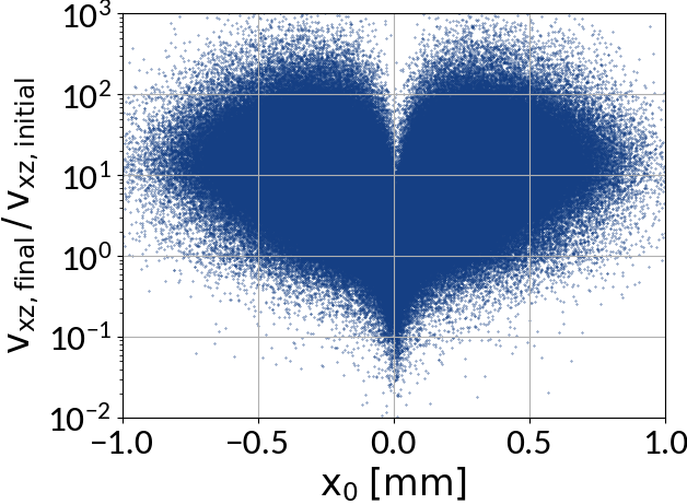
What about particles that have their velocity decreased?
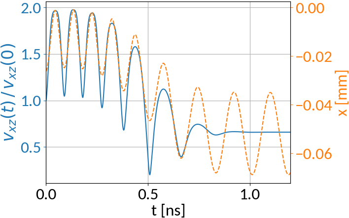
\vec{x}_0 = \begin{pmatrix} -0.097\sigma_x \\ -0.090\sigma_y \\ -0.5\sigma_z \end{pmatrix}, \vec{v}_0 = \begin{pmatrix} 85079 \\ 425128 \\ -897701 \end{pmatrix} \frac{m}{s}
Initial parameters:
\vec{x}_0 = \begin{pmatrix} 1\sigma_x \\ 0 \\ -0.5\sigma_z \end{pmatrix}, \vec{v}_0 = \begin{pmatrix} 707214 \\ 707214 \\ -707214 \end{pmatrix} \frac{m}{s}
Compare with particle that has its velocity increased:
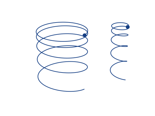
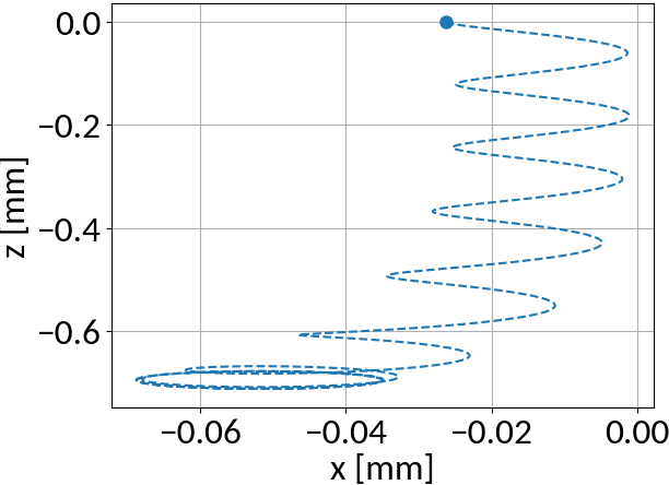
Gyromotion
Space-charge region
Detector region
Electron motion is different for two distinct regions:
- Space-charge region: beam field influences velocity
- Detector region: pure gyromotion without beam field influence
Distortion through gyromotion
Gyromotion is parametrized via
\begin{aligned}
x(t) &= \frac{v_{x0}}{\omega}\sin(\omega t) + \frac{v_{z0}}{\omega}\cos(\omega t) + \left( x_0 - \frac{v_{z0}}{\omega} \right) \\
&\\
z(t) &= -\frac{v_{x0}}{\omega}\cos(\omega t) + \frac{v_{z0}}{\omega}\sin(\omega t) + \left( z_0 + \frac{v_{x0}}{\omega} \right)
\end{aligned}
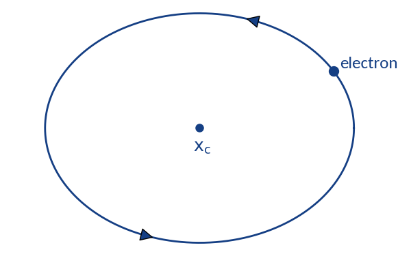
Particle spirals around
and will be detected in the range
x_c = x_0 - \frac{v_{z0}}{\omega}
x_c \pm \frac{\sqrt{v_{x0}^2 + v_{z0}^2}}{\omega}

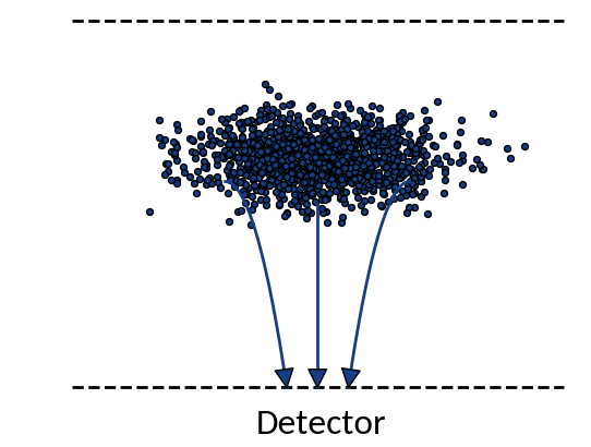
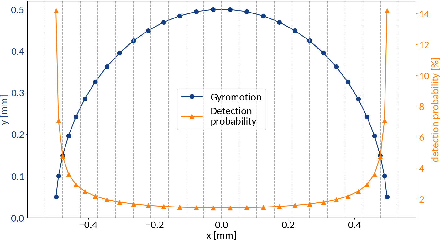
Detection probabilities
Provided that the moment of detection is random, the gyromotion of electrons gives rise to probabilities of being detected at a specific position.
p(x) \propto \lvert \lim_{\Delta x \rightarrow 0} \frac{1}{\Delta x} \int_{x}^{x + \Delta x} ds \rvert = \frac{1}{\sqrt{R^2 - (x - x_c)^2}}
Applying the limit results in divergence at the "edges" of the motion, so the expression is only valid for the center. For real profiles however we can work with a discretized version of the abovementioned relation.
small statistics
Summary of displacements
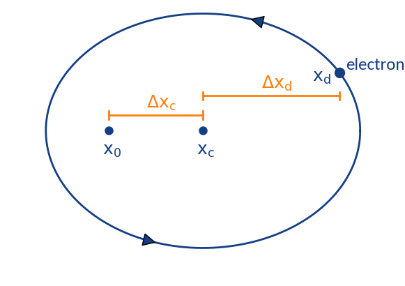
- position at ionization
- gyration center (detector region)
- position of detection
x_0
x_c
x_d
Two types of displacement:
- : Depends on initial z-velocity, transverse electric field, ExB-drift by long. electric field
- : Displacement due to gyration motion; stochastic displacement
\Delta x_c
\Delta x_d
Analytical description?
In principal z-velocities are relatively small (shift ~ 10 μm; ionized electrons are mainly scattered in transverse direction), the longitudinal electric field can be neglected and the center shift due to the transverse electric field is around a few micrometers which is small compared to the magnitude of the gyro-motion.
Describing the gyro-distortion via point-spread-functions is however not possible because the gyro-velocity increase is not uniform along the profile.
Simulating the process
Virtual-IPM simulation tool was used to generate the data
| Parameter | Range | Step size |
|---|---|---|
| Bunch pop. [1e11] | 1.1 -- 2.1 ppb | 0.1 ppb |
| Bunch width (1σ) | 270 -- 370 μm | 5 μm |
| Bunch height (1σ) | 360 -- 600 μm | 20 μm |
| Bunch length (4σ) | 0.9 -- 1.2 ns | 0.05 ns |
Protons
6.5 TeV
4kV / 85mm
0.2 T
= 21,021 cases | 5h / case | 12 yrs | Good thing there are computing clusters :-)
Physics models
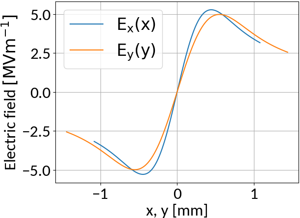
Analytical expression for the electric field of a two-dimensional Gaussian charge distribution
🡒 Longitudinal field is neglected; justifiable for highly relativistic beam
🡒 Magnetic field is considered
M. Bassetti and G.A. Erskine, "Closed expression for the electrical field of a two-dimensional Gaussian charge", CERN-ISR-TH/80-06, 1980
Double differential cross section for relativistic incident particles
A. Voitkiv et al, "Hydrogen and helium ionization by relativistic projectiles in collisions with small momentum transfer", J.Phys.B: At.Mol.Opt.Phys, vol.32, 1999
Uniform electric and magnetic guiding fields
Simulated profiles
Simulation outputs particle parameters as csv data frame
Summarize initial and final positions into 1 μm histograms ranging [-10, 10] mm
Rebin to 55 μm (silicon pixel detector) and 100 μm (optical acquisition system)
Bunch population and bunch length
&
Data preparation
| ppb | 4σz | f [1] | ... | f [n] | i [1] | ... | i [n] |
Data
Measured profile
Beam profile
Input
Output
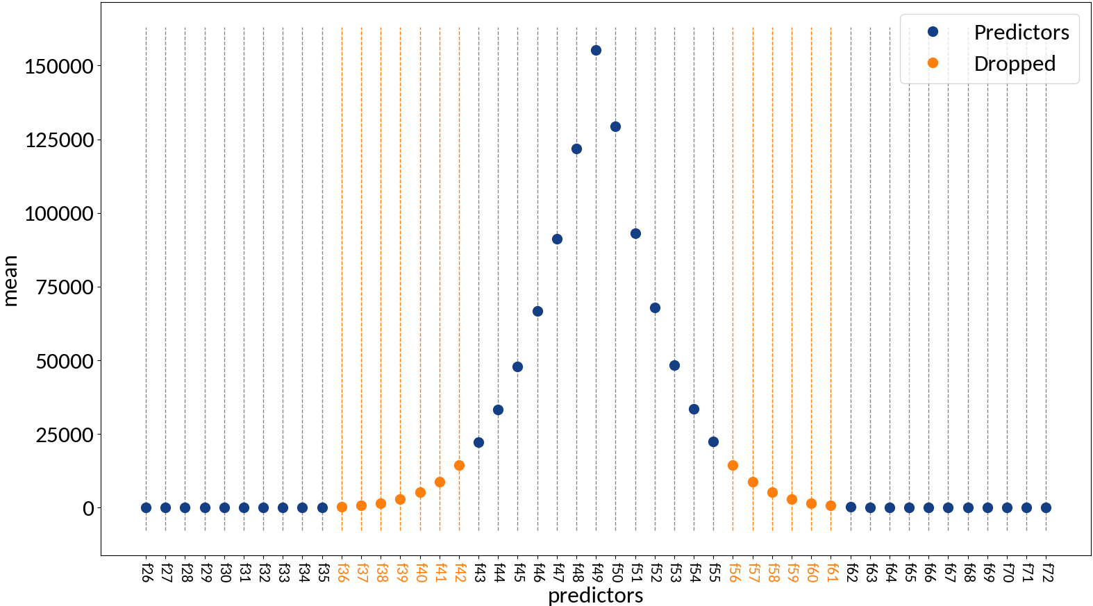
Drop zero variance variables (as they don't provide any information)
Rescale data to have zero mean and unit variance:
x \rightarrow (x - \mu) / \sigma
Compute σ from profile
Optionally rescale
(\;\;\;\;\;\;)
Train, Test, Validate
Divide the machine "learning" into three stages and corresponding data sets:
Training

Validation

Testing

This data set is used to derive rules from the data, i.e. to fit the model (e.g. polynomial fit). Split size ~ 60%.
This data set is used to ensure that the model generalizes well to unseen data, between multiple iterations of hyper-parameter tuning (e.g. polynomial degree) and model selection. Split size ~ 20%.
This data set is used for evaluating the performance of the final model (in order to prevent "tuning-bias"). Split size ~ 20%.
Evaluating performance
Explained variance
1 - \frac{Var\left[ y_{true} - y_{pred} \right]}{Var\left[ y_{true} \right]}
Mean squared error
\frac{1}{N}\Sigma\left( y_{true} - y_{pred} \right)^2
R2-score
1 - \frac{\Sigma\left( y_{true} - y_{pred} \right)^2}{\Sigma\left( y_{true} - \mu_{true} \right)^2}

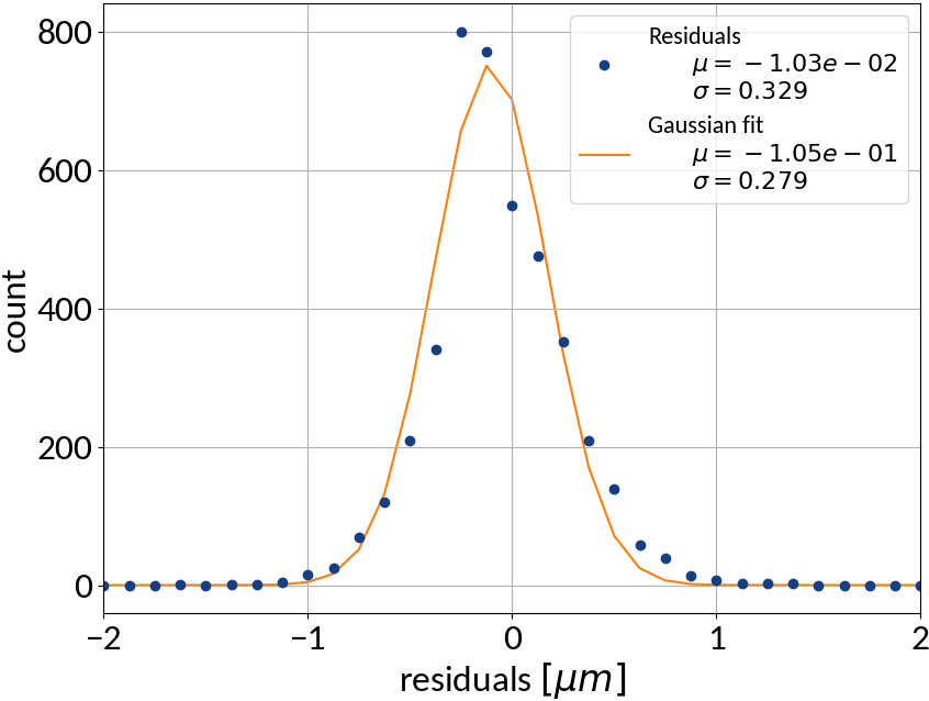
Anscombe's quartet
Similar mean, variance and R2 (approx.)
Residuals plot is important
Visualization helps in assessing the quality of a model
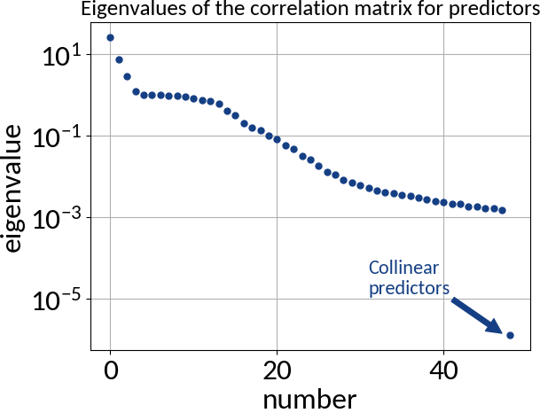
Multivariable linear regression
\sigma_x = \vec{\beta}^{\,T}\vec{x} + b + \epsilon
Requirements:
- Predictors are error-free
- Absence of multi-collinearity among the predictors
predictors
intercept
error term
Multivariable linear regression - Results
| Explained variance | 0.99972 |
| R2-score | 0.99972 |
| Mean squared error | 0.25212 |
\mu m^2
Kernel ridge regression
Twofold extension of "classical" linear regression:
- Uses ridge regularization for the learned weights (L2-norm)
- Employs the "Kernel trick"
L = \frac{1}{2}\Sigma_i \left( y_{i, true} - y_{i, pred} \right)^2 + \frac{1}{2}\lambda\left|\left|w\right|\right|^2
L2 "ridge" regularization:
Adding the norm of the weights to the loss function puts a penalty on the weights.
Strength of penalization can be adjusted.
Regularization term prevents overfitting
The Kernel Trick
Features can't be separated by a linear function ...
... at least not in two-dimensional space.
Define a mapping, for example:
\begin{aligned}
& K: \mathbb{R}^2 \rightarrow \mathbb{R}^3 \\
& K(x, y) = \left( x, y, x^2 + y^2 \right)
\end{aligned}
Now the space in which K maps may be very high dimensional, so computing the corresponding vectors is expensive.
The trick is to express the dot product of K(x, y) in terms of the initial vectors (x, y) 🡒 no need to compute K(x, y).
Kernel ridge regression - Results
Polynomial kernel
K(x, y) = \left(x^Ty + c\right)^2
Radial basis function kernel
K(x, y) = \exp\left( -\gamma || x - y || \right)
\alpha = 0.001
degree = 2
\alpha = 0.001
\gamma = 0.0002
| Poly kernel | RBF kernel | |
| Explained variance | 0.99983 | 0.99974 |
| R2-score | 0.99983 | 0.99974 |
| Mean squared error | 0.15074 | 0.23331 |

\mu m^2
\mu m^2
Support Vector Machine

- Originally developed for classification tasks
- Find a linear separation of two classes with maximum margin between them
\hat{y} = sgn\left( \sum_i \alpha_i y_i \vec{x}_i\cdot\hat{\vec{x}} + b \right)
prediction
learned weights
class labels
training data
intercept of hyperplane
Fitting and predicting only depends on dot products of feature vectors, so we can use the kernel trick
Support Vector Regression
SVM
hinge loss
SVR
ε-insensitive loss
\max\left( 0, 1 - y_i\cdot f(x_i) \right)
\max\left( 0, \lvert y_i - f(x_i) \rvert - \epsilon \right)
The fitted model is similar to Kernel Ridge Regression but the loss function is different (KRR uses ordinary least squares)
y(x) = \sum_i \alpha_i K(x_i, x) + b
Support Vector Regression - Results
| Explained variance | 0.99985 |
| R2-score | 0.99985 |
| Mean squared error | 0.13527 |
\begin{aligned}
K &= \textrm{RBF} \\
\gamma &= 10^{-4} \\
\epsilon &= 10^{-8} \\
C &= 10^3
\end{aligned}
\mu m^2
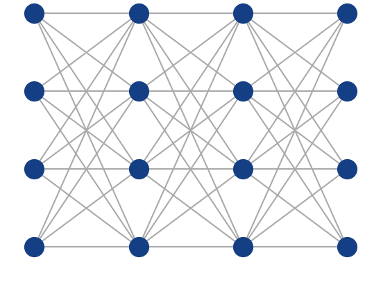
Artificial Neural Networks
Inspired by the human brain, many "neurons" linked together
Input layer
Weights
Bias
Apply non-linearity, e.g. sigmoid, tanh
Perceptron
y(x) = \sigma\left( W\cdot x + b \right)
Multi-Layer Perceptron
Deep Learning

What means deep?
Usually two or more hidden layers.
Using fully connected layers, the number of parameters can grow quite large (e.g. one of the MNIST top classifiers uses 6 layers = 11,972,510 parameters).
All those parameters are adjusted using the training data.
How deep networks learn
Define a loss function that assesses how good the network's predictions are, e.g. mean squared error:
L = \sum_i \left( y_i - \hat{y_i} \right)^2
Compute the gradient of the loss with respect to network parameters, e.g. Gradient Descent or Adam (uses "momentum").
w \rightarrow w - \eta\frac{\partial L}{\partial w}
Update the network's parameters by applying the gradient with a learning rate:
Deep Learning Frameworks


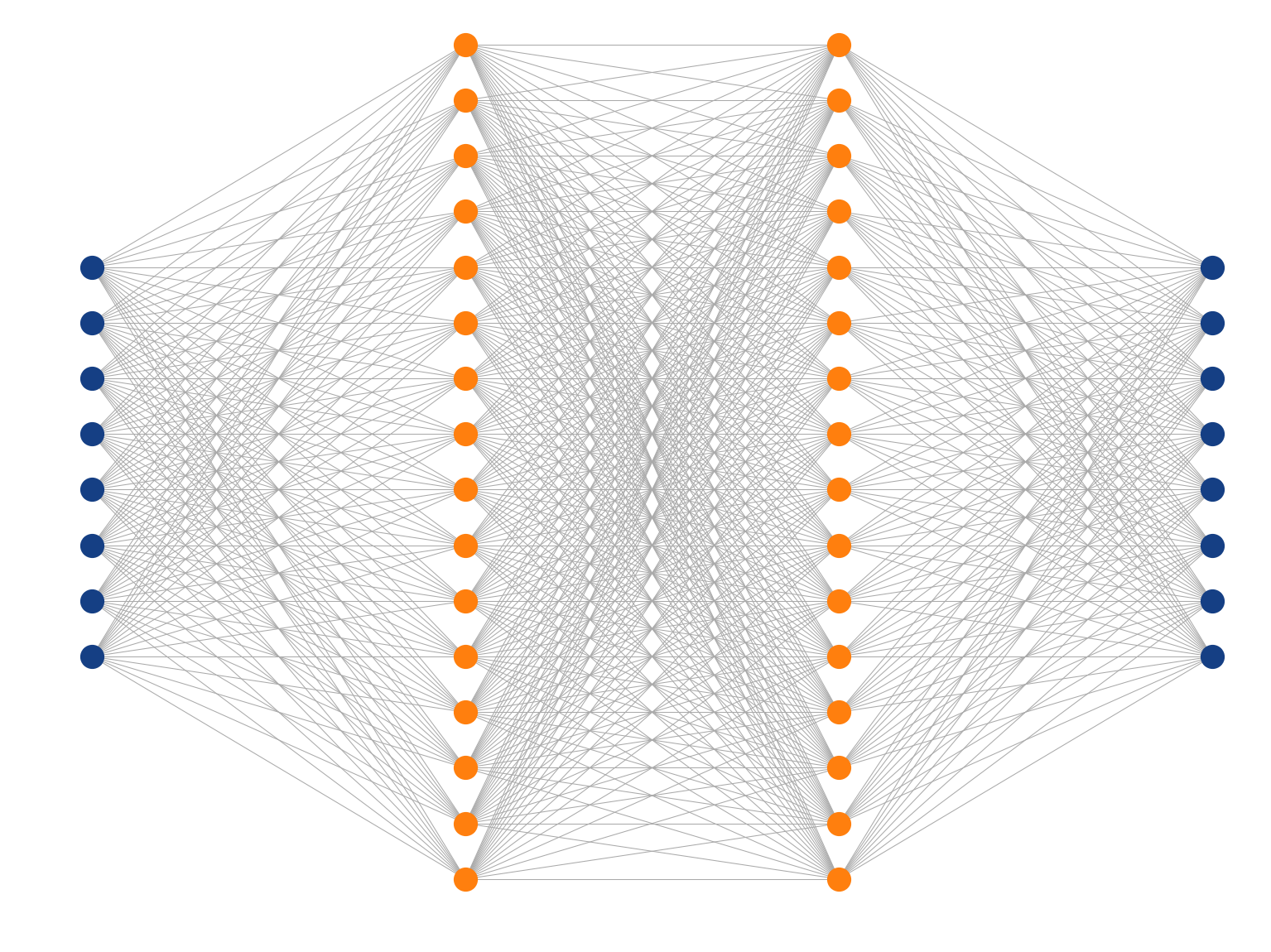
ANN Architecture
IDense = partial(Dense, kernel_initializer=VarianceScaling())

# Create feed-forward network.
model = Sequential()

# Since this is the first hidden layer we also need to specify
# the shape of the input data (49 predictors).
model.add(IDense(200, activation='relu', input_shape=(49,))
model.add(IDense(170, activation='relu'))
model.add(IDense(140, activation='relu'))
model.add(IDense(110, activation='relu'))

# The network's output (beam sigma). This uses linear activation.
model.add(IDense(1))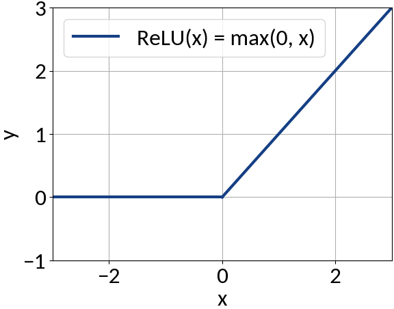
Activation function
Fully-connected (dense) feed-forward (sequential) architecture
ANN Learning
model.compile(
    optimizer=Adam(lr=0.001),
    loss='mean_squared_error'
)

model.fit(
    x_train, y_train,
    batch_size=8, epochs=100, shuffle=True,
    validation_data=(x_val, y_val)
)
D. Kingma and J. Ba, "Adam: A Method for Stochastic Optimization", arXiv:1412.6980, 2014
Other possible optimizers are Stochastic Gradient Descent for example.
Batch learning
- Training is an iterative procedure
- Need to go through the data set multiple times (= 1 epoch)
- Weight updates are performed in batches (🡒 batch size)
After each epoch compute the loss on the validation data in order to prevent overfitting
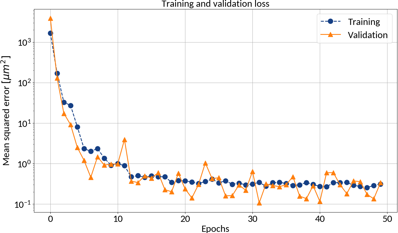
Could apply early stopping
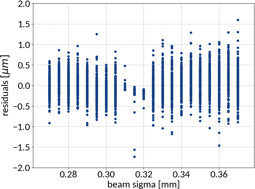
ANN - Results
| Explained variance | 0.99988 |
| R2-score | 0.99988 |
| Mean squared error | 0.10959 |
\mu m^2
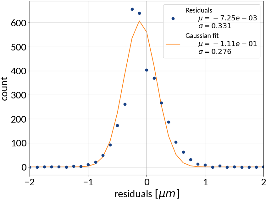
Summary of model performance
| μ (res.) | σ (res.) | R2-score | MSE | |
|---|---|---|---|---|
| Linear | 0.000213 | 0.502 | 0.99972 | 0.22512 |
| KRR | 0.00590 | 0.388 | 0.99983 | 0.15074 |
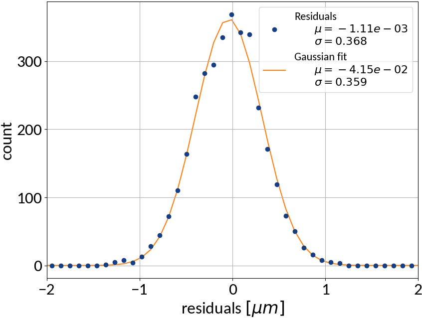
| SVR | -0.00111 | 0.368 | 0.99985 | 0.13527 |
| ANN | -0.00725 | 0.331 | 0.99988 | 0.10959 |
Values are given in units of
\mu m, \mu m^2 (\textrm{MSE}).
- Artificial neural network (multi-layer perceptron) showed the best performance
- Although the residuals changed with sigma, no bias occurred and beam sigma is expected to be in the center of the range anyway
Performance on test data
| Explained variance | 0.99988 |
| R2-score | 0.99988 |
| Mean squared error | 0.10815 |
\mu m^2
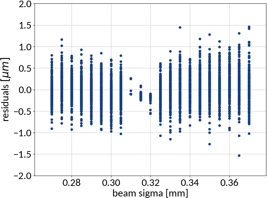
Using ANN
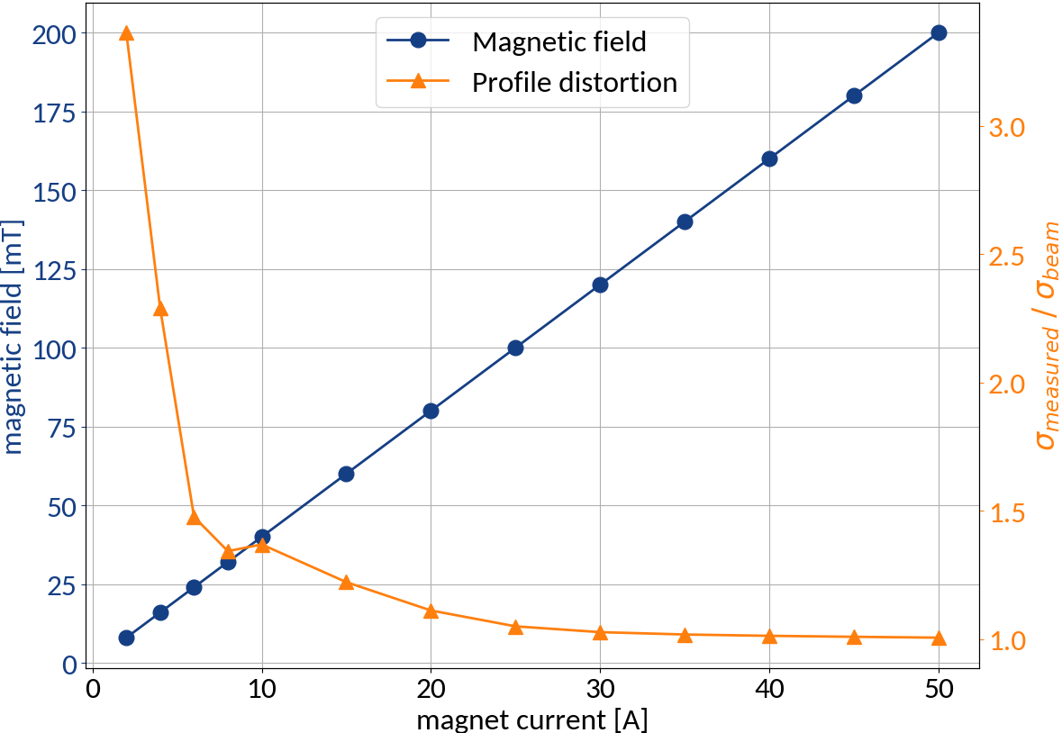
Measuring space-charge induced profile distortion
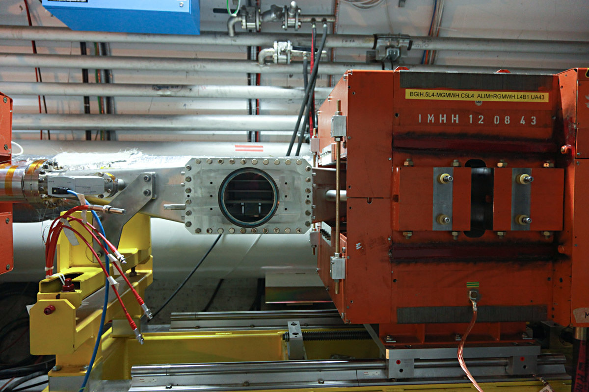
Measurements taken at CERN / SPS / BGI-H
| Electric field | 4 kV / 85 mm |
| Magnetic field | 0.2 T (50A) |
At the max. magnetic field no profile distortion occurs, but we can reduce the magnet current to make that happen
Acquisition system:
MCP + Phosphor + Camera
| Protons | |
|---|---|
| Energy | 400 GeV |
| Bunch pop. | 2.859e11 |
| Beam width (1σ) | 0.835 mm |
| Beam height (1σ) | 0.451 mm |
| Bunch length (4σ) | 1.6 ns |
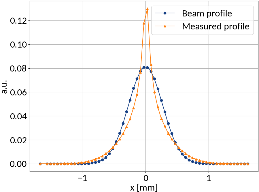
The Measurements
Taking into account:
- Pixel-to-mm calibration
- Camera rotation
- Optical PSF (~ 130 μm)

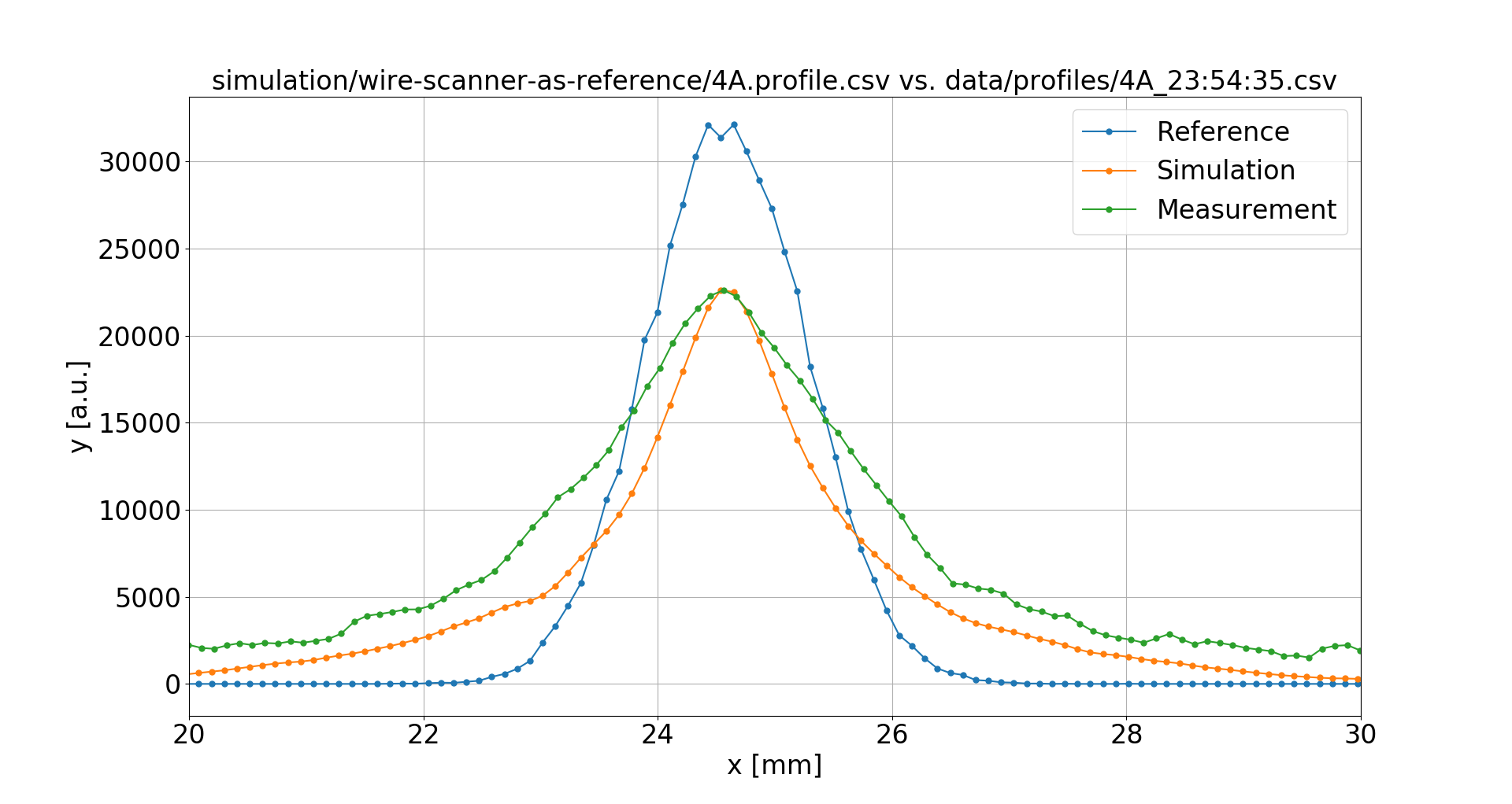
Wire Scanners were used to obtain undistorted reference profiles, however only the sigma values from fit were available
Bad luck with the RNG
4 A
16 mT
20 A
80 mT
What about the PSF?
Trying a 520 μm point-spread function instead:
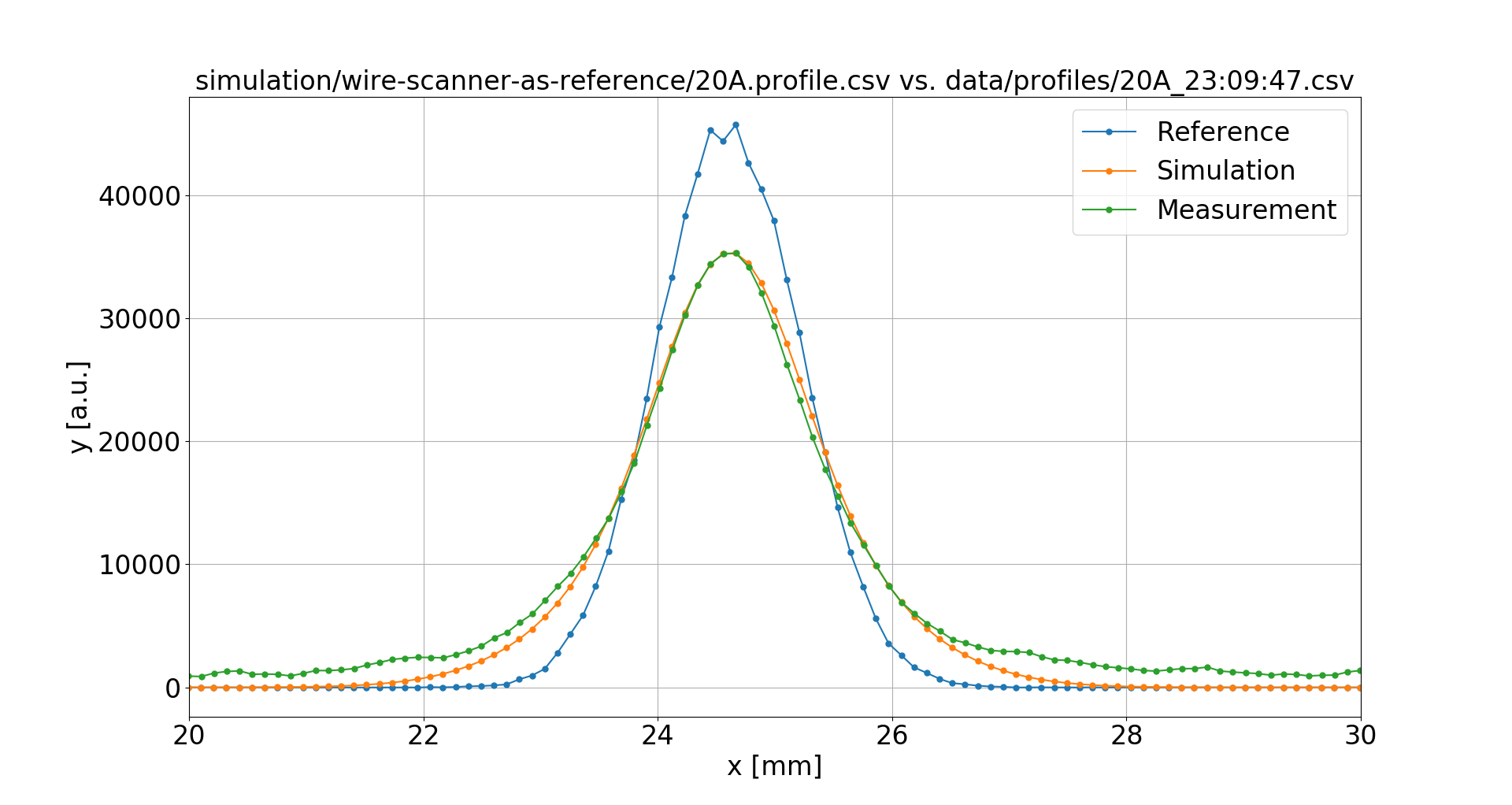

This resolves the deviations for all magnetic field values.
4 A
16 mT
20 A
80 mT
However such a large PSF is difficult to explain.
Next steps
Hyper-parameter tuning is tedious but there are helpful tools
Collect more data from measurements
Test the method against measured reference profiles (e.g. from Wire Scanners)
Test the method with "unclean" data (e.g. noise added, PSF applied)
from sklearn.model_selection \
    import GridSearchCV

from autosklearn.regression \
    import AutoSklearnRegressor
Investigate the effect of different profile binnings, i.e. different number of predictors
All models are wrong but some are useful.
- George Box (1978)
Piqued your interest?
Icons by icons8.
Please find more information at https://ipmsim.gitlab.io/IPMSim/
The data presented in this talk was generated with Virtual-IPM
Using Machine Learning for IPM profile reconstruction
By Dominik Vilsmeier
Using Machine Learning for IPM profile reconstruction
Operations Beam Physics and Techniques Salon, GSI Helmholtz Centre for Heavy Ion Research (Darmstadt, Germany), February 20th 2018


