

federica bianco PRO
astro | data science | data for good
dr.federica bianco | fbb.space | fedhere | fedhere
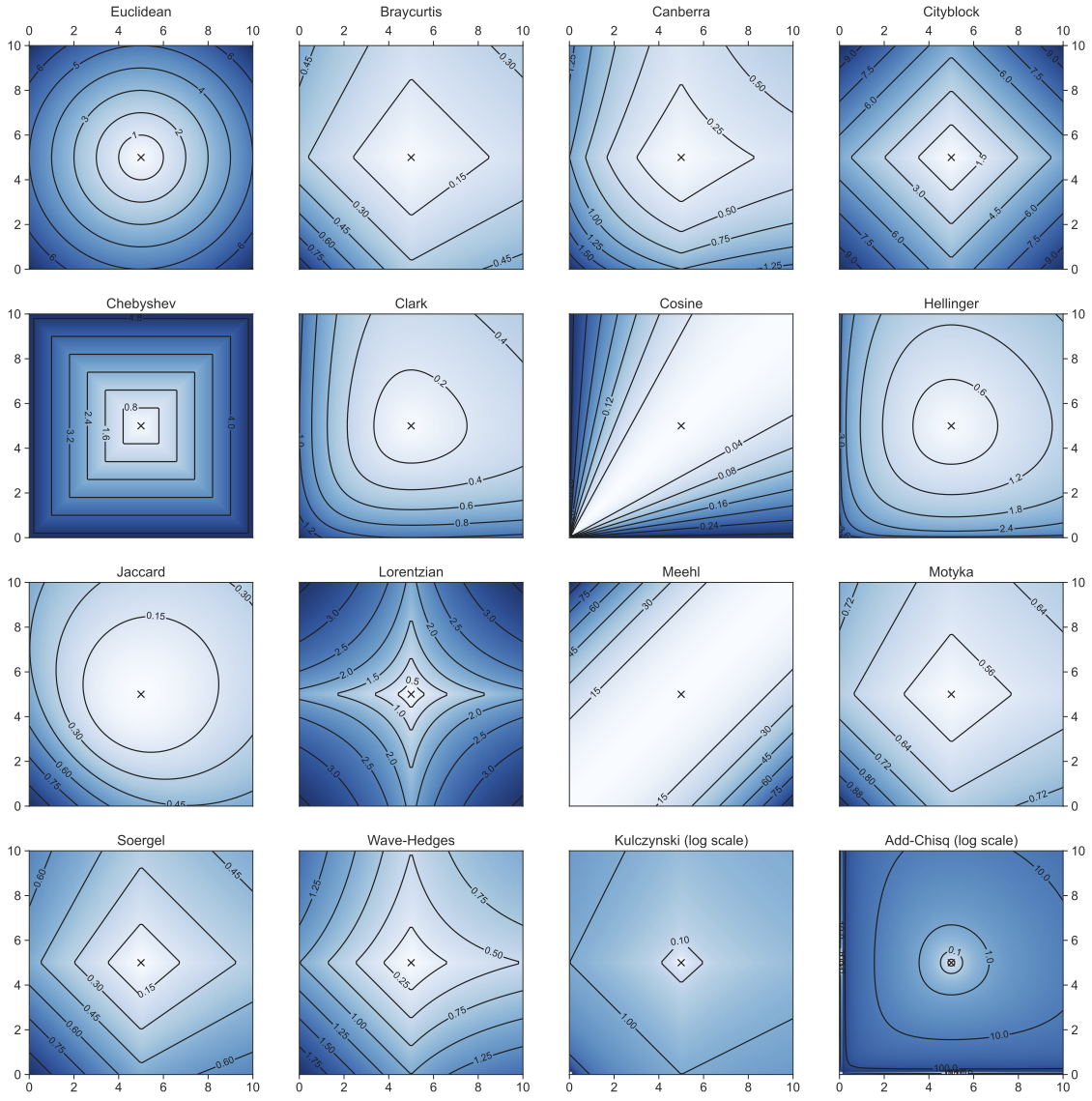
distances
this slide deck
0
Machine Learning
unsupervised learning
identify features and create models that allow to understand structure in the data
unsupervised learning
identify features and create models that allow to understand structure in the data
supervised learning
extract features and create models that allow prediction where the correct answer is known for a subset of the data
Calculate the distance d to all known objects

Select the k closest objects

Assign the most common among the k classes:
# k = 1
d = distance(x, trainingset)
C(x) = C(trainingset[argmin(d)])Calculate the distance d to all known objects Select the k closest objects
Classification:
Assign the most common among the k classes
Regression:
Predict the average (median) of the k target values
Good
non parametric
very good with large training sets
Cover and Hart 1967: As n→∞, the 1-NN error is no more than twice the error of the Bayes Optimal classifier.
Good
non parametric
very good with large training sets
Cover and Hart 1967: As n→∞, the 1-NN error is no more than twice the error of the Bayes Optimal classifier.
Let xNN be the nearest neighbor of x.
For n→∞, xNN→x(t) => dist(xNN,x(t))→0
Theorem: e[C(x(t)) = C(xNN)]< e_BayesOpt
e_BayesOpt = argmaxy P(y|x)
Proof: assume P(y|xt) = P(y|xNN)
(always assumed in ML)
eNN = P(y|x(t)) (1−P(y|xNN)) + P(y|xNN) (1−P(y|x(t))) ≤
(1−P(y|xNN)) + (1−P(y|x(t))) =
2 (1−P(y|x(t)) = 2ϵBayesOpt,
Good
non parametric
very good with large training sets
Not so good
it is only as good as the distance metric
If the similarity in feature space reflect similarity in label then it is perfect!
poor if training sample is sparse
poor with outliers
Wine Example
PROS:
Because the model does not need to provide a global optimization the classification is "on-demand".
This is ideal for recommendation systems: think of Netflix and how it provides recommendations based on programs you have watched in the past.
CONS:
Need to store the entire training dataset (cannot model data to reduce dimensionality).
Training==evaluation => there is no possibility to frontload computational costs
Evaluation on demand, no global optimization - doesn’t learn a discriminative function from the training data but “memorizes” the training dataset instead.
1
Any algorithm that fulfills the following conditions
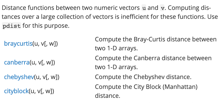
Minkowski family of distances
Minkowski family of distances
N features (dimensions)
Minkowski family of distances
Manhattan: p=1
features: x, y
Minkowski family of distances
Manhattan: p=1
features: x, y
Minkowski family of distances
Euclidean: p=2
features: x, y
Minkowski family of distances
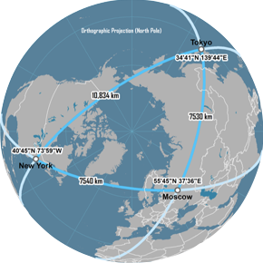
Great Circle distance
features
latitude and longitude
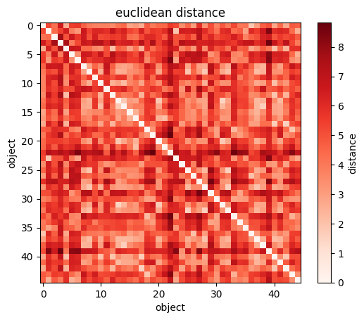
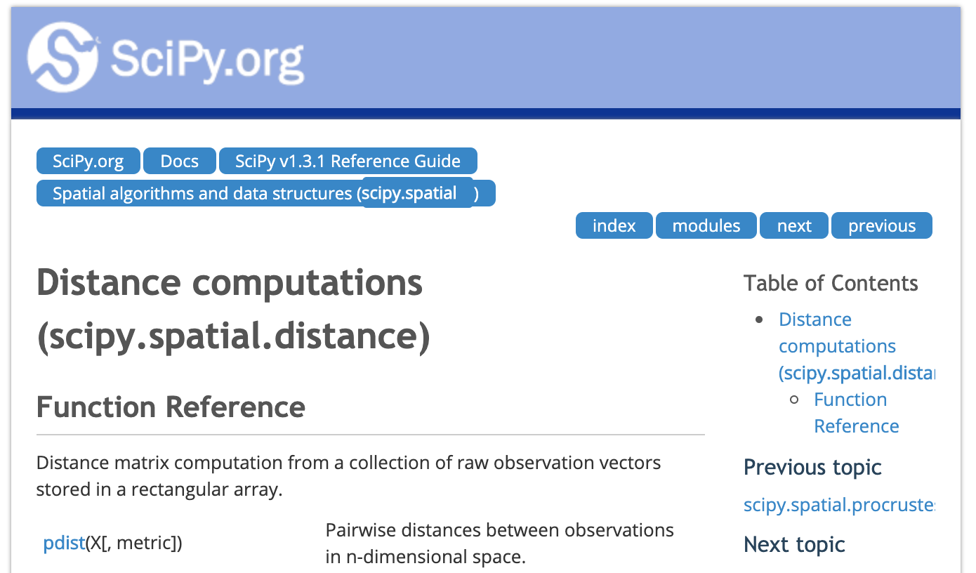
import scipy as sp

sp.spatial.distance.pdist(X) # the pairwise distance: returns (N**2  - N )/2 values for N objects

sp.spatial.distance.squareform(sp.spatial.distance.pdist(wines[["Alcohol", "Magnesium"]]))
#returns the NXN matrix of distances

plt.imshow(sp.spatial.distance.squareform(sp.spatial.distance.pdist(wines[["Alcohol", "Magnesium"]])))
#you can visualize the NXN matrix


plt.xlabel("wine")
plt.ylabel("wine");
plt.colorbar(label="distance");
import scipy as sp
sp.spatial.distance.pdist(X) # the pairwise distance: returns (N**2 - N )/2 values for N objects
sp.spatial.distance.squareform(sp.spatial.distance.pdist(wines[["Alcohol", "Magnesium"]]))
#returns the NXN matrix of distances
plt.imshow(sp.spatial.distance.squareform(sp.spatial.distance.pdist(wines[["Alcohol", "Magnesium"]])))
#you can visualize the NXN matrix
plt.xlabel("wine")
plt.ylabel("wine");
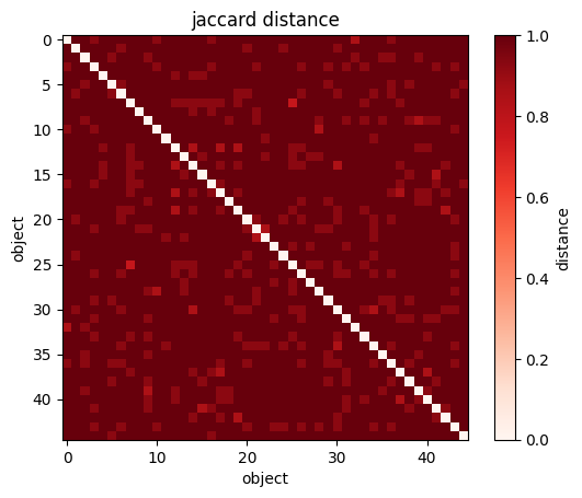
plt.colorbar(label="distance");import scipy as sp
sp.spatial.distance.pdist(X) # the pairwise distance: returns (N**2 - N )/2 values for N objects
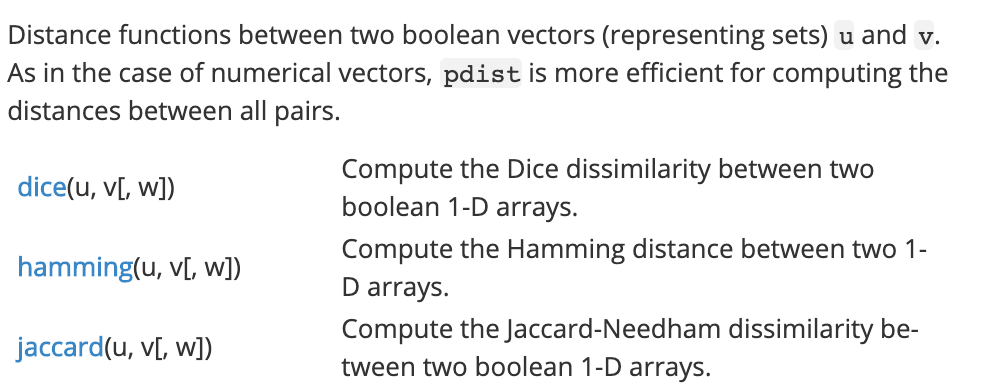
sp.spatial.distance.squareform(sp.spatial.distance.pdist(wines[["Alcohol", "Magnesium"]],
metric='jaccard'))
#returns the NXN matrix of distances
plt.imshow(sp.spatial.distance.squareform(sp.spatial.distance.pdist(wines[["Alcohol", "Magnesium"]])))
#you can visualize the NXN matrix
plt.xlabel("wine")
plt.ylabel("wine");
plt.colorbar(label="distance");#Great Circle Distance in the sky
import astropy.units as u
from astropy.coordinates import SkyCoord
#The on-sky separation can be computed with the astropy.coordinates.BaseCoordinateFrame.separation()
#or astropy.coordinates.SkyCoord.separation() methods,
#which computes the great-circle distance (not the small-angle approximation):
c1 = SkyCoord('5h23m34.5s', '-69d45m22s', frame='icrs')
c2 = SkyCoord('0h52m44.8s', '-72d49m43s', frame='fk5')
sep = c1.separation(c2)Angle 20.74611448 deg
from shapely.geometry import Point
import geopandas as gpd
pnt1 = Point(80.99456, 7.86795)
pnt2 = Point(80.97454, 7.872174)
points_df = gpd.GeoDataFrame({'geometry': [pnt1, pnt2]}, crs='EPSG:4326')
points_df = points_df.to_crs('EPSG:5234')
points_df2 = points_df.shift() #We shift the dataframe by 1 to align pnt1 with pnt2
points_df.distance(points_df2)
https://www.codedrome.com/calculating-great-circle-distances-in-python/
https://pypi.org/project/great-circle-calculator/
from math import radians, degrees, sin, cos, asin, acos, sqrt
def great_circle(lon1, lat1, lon2, lat2):
    lon1, lat1, lon2, lat2 = map(radians, [lon1, lat1, lon2, lat2])
    return 6371 * (acos(sin(lat1) * sin(lat2) + cos(lat1) *
cos(lat2) * cos(lon1 - lon2))) #kmUses presence/absence of features in data
: number of features in neither
: number of features in both
: number of features in i but not j
: number of features in j but not i
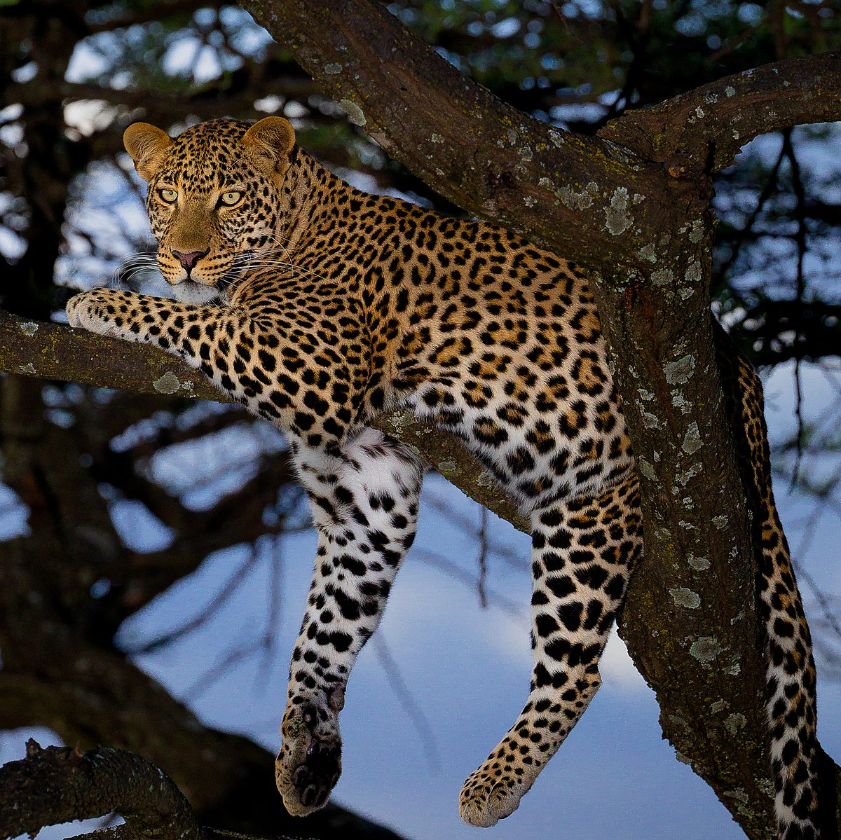
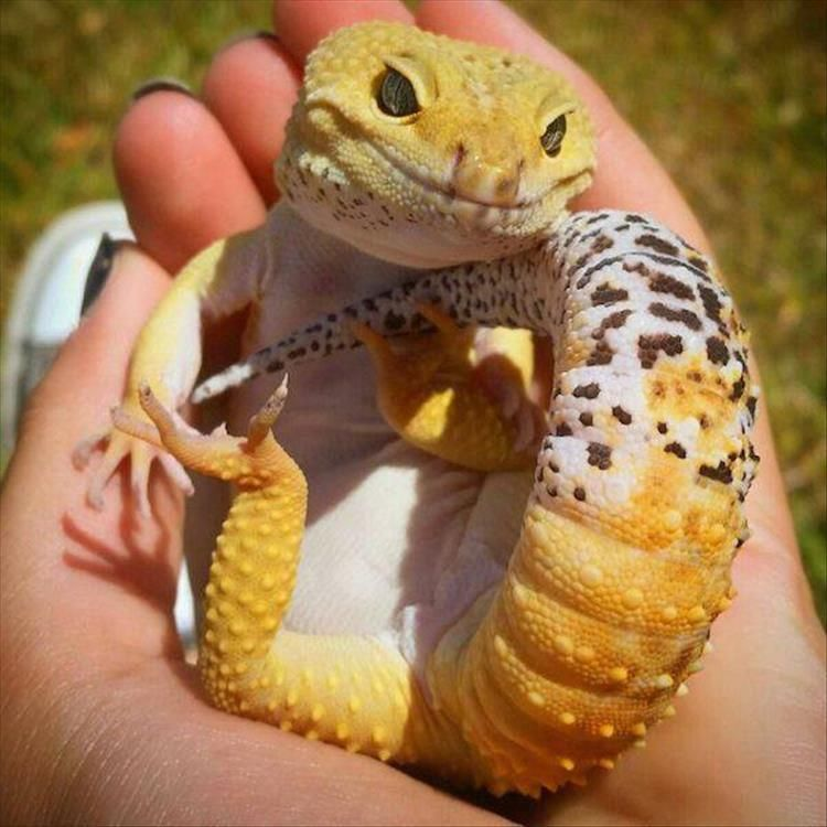
What is the distance between a leopard and a lizard?
- they both have tails
- only lizards have scales
- neither have wings
Uses presence/absence of features in data
: number of features in neither
: number of features in both
: number of features in i but not j
: number of features in j but not i
What is the distance between a leopard and a lizard?
- they both have tails
- only lizards have scales
- neither have wings
| 1 | 0 | sum | |
|---|---|---|---|
| 1 | M11 | M10 | M11+M10 |
| 0 | M01 | M00 | M01+M00 |
| sum | M11+M01 | M10+M00 | M11+M00+M01+ M10 |
observation i
}
}
| 0 | sum | ||
|---|---|---|---|
| 1 | M10 | M11+M10 | |
| 0 | M01 | M00 | M01+M00 |
| sum | M11+M01 | M10+M00 | M11+M00+M01+ M10 |
1
1
1
0
Simple Matching Distance
Uses presence/absence of features in data
: number of features in neither
: number of features in both
: number of features in i but not j
: number of features in j but not i
Simple Matching Coefficient
or Rand similarity
| 1 | 0 | sum | |
|---|---|---|---|
| 1 | M11 | M10 | M11+M10 |
| 0 | M01 | M00 | M01+M00 |
| sum | M11+M01 | M10+M00 | M11+M00+M01+ M10 |
observation i
observation j
}
}
| 0 | sum | ||
|---|---|---|---|
| 1 | M11 | M10 | M11+M10 |
| 0 | M01 | M00 | M01+M00 |
| sum | M11+M01 | M10+M00 | M11+M00+M01+ M10 |
1
1
1
0
lizard/leopard
Jaccard similarity
Jaccard distance
| 1 | 0 | sum | |
|---|---|---|---|
| 1 | M11 | M10 | M11+M10 |
| 0 | M01 | M00 | M01+M00 |
| sum | M11+M01 | M10+M00 | M11+M00+M01+ M10 |
observation i
observation j
}
}
lizard/leopard
Jaccard similarity
Jaccard distance
| 1 | 0 | sum | |
|---|---|---|---|
| 1 | M11 | M10 | M11+M10 |
| 0 | M01 | M00 | M01+M00 |
| sum | M11+M01 | M10+M00 | M11+M00+M01+ M10 |
observation i
observation j
}
}
Jaccard similarity
Application to Deep Learning for image recognition
Convolutional Neural Nets
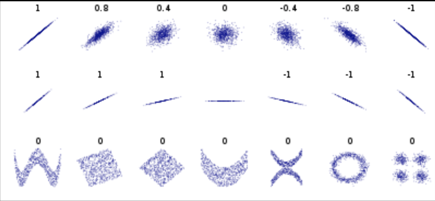
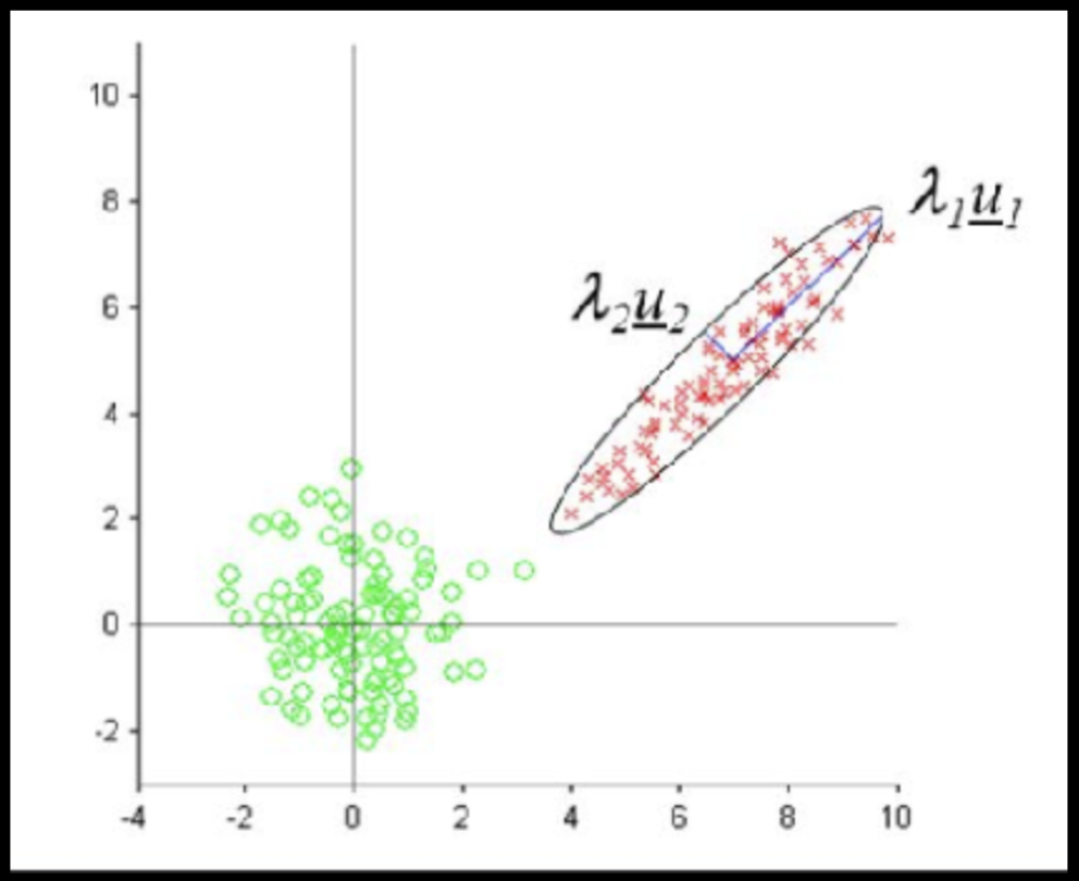
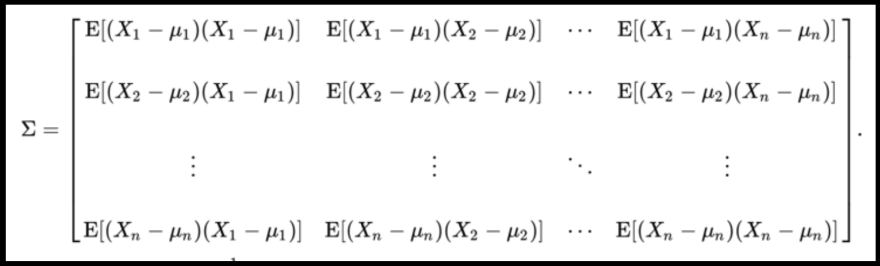
Data can have covariance (and it almost always does!)
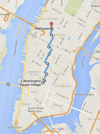
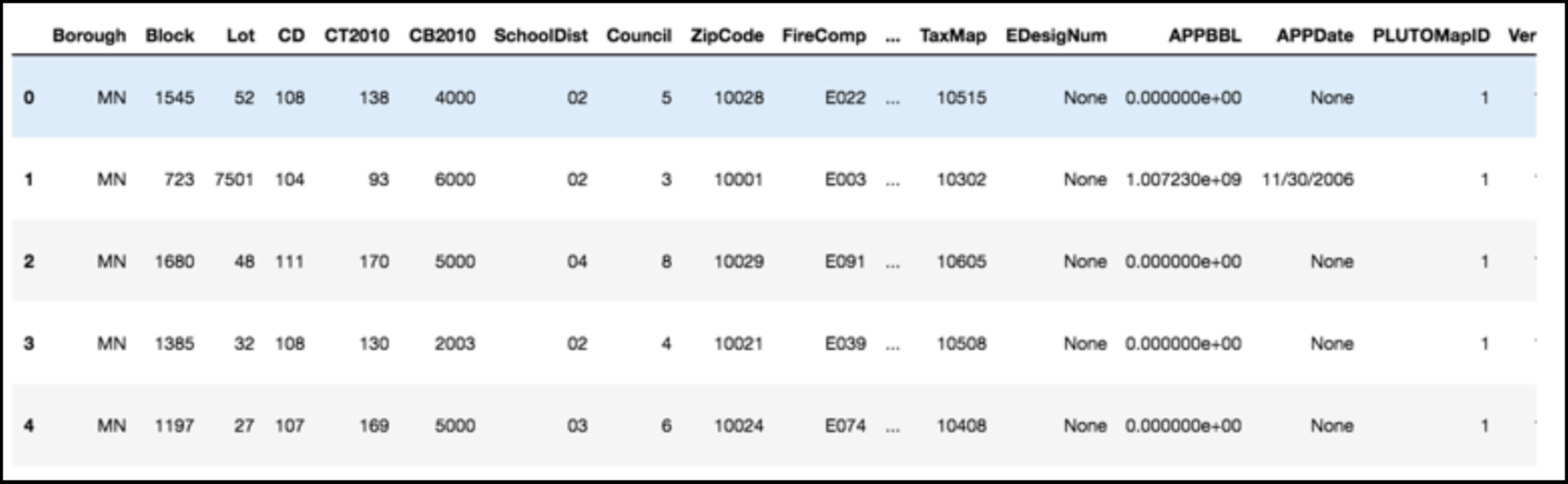
PLUTO Manhattan data (42,000 x 15)
axis 1 -> features
axis 0 -> observations
Data can have covariance (and it almost always does!)
PLUTO Manhattan data (42,000 x 15)
axis 1 -> features
axis 0 -> observations
COVARIANCE = correlation / variance
Data can have covariance (and it almost always does!)
Data can have covariance (and it almost always does!)
Pearson's correlation (linear correlation)
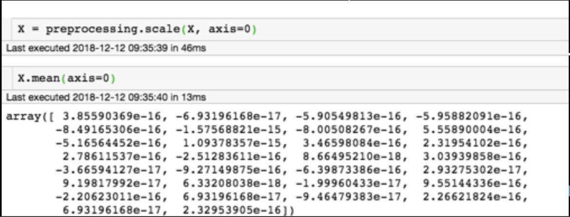
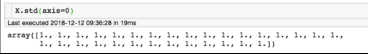
Generic preprocessing... WHY??
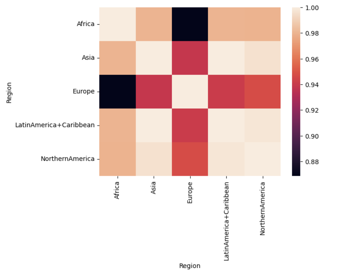
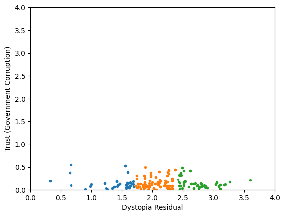
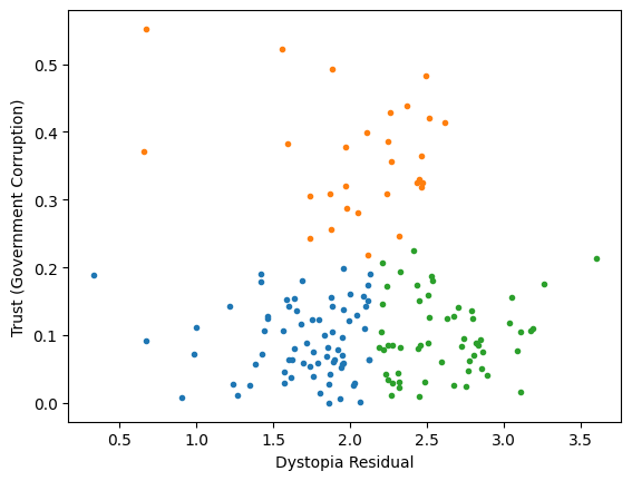
Worldbank Happyness Dataset https://github.com/fedhere/MLPNS_FBianco/blob/main/clustering/happiness_solution.ipynb
Clustering without scaling:
only the variable with more spread matters
Skewed data distribution:
std(x) ~ range(y)
Generic preprocessing... WHY??
Worldbank Happyness Dataset https://github.com/fedhere/MLPNS_FBianco/blob/main/clustering/happiness_solution.ipynb
Clustering without scaling:
only the variable with more spread matters
Skewed data distribution:
std(x) ~ range(y)
Clustering
Classifying &
regression
Unsupervised learning
Supervised learning
unsupervised vs supervised learning
Data that is not correlated appear as a sphere in the Ndimensional feature space
Data can have covariance (and it almost always does!)
ORIGINAL DATA
STANDARDIZED DATA
Generic preprocessing
Generic preprocessing... WHY??
Worldbank Happyness Dataset
Classification/Clustering without scaling:
only the variable with more spread matters
Generic preprocessing... WHY??
Worldbank Happyness Dataset
Classification/Clustering without scaling:
only the variable with more spread matters
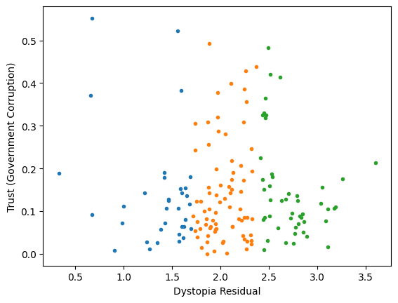
Classification/Clustering
after scaling:
both variables matter equally
Data that is not correlated appear as a sphere in the Ndimensional feature space
Data can have covariance (and it almost always does!)
ORIGINAL DATA
STANDARDIZED DATA
Generic preprocessing
Generic preprocessing
for each feature: divide by standard deviation and subtract mean
Generic preprocessing: most commonly, we will just correct for the spread and centroid
The term "whitening" refers to white noise, i.e. noise with the same power at all frequencies"
PLUTO Manhattan data (42,000 x 15) correlation matrix
axis 1 -> features
axis 0 -> observations
Data can have covariance (and it almost always does!)
PLUTO Manhattan data (42,000 x 15) correlation matrix
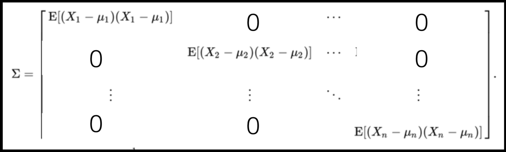
A covariance matrix is diagonal if the data has no correlation
Data can have covariance (and it almost always does!)
Full On Whitening
find the matrix W that diagonalized Σ
from zca import ZCA
import numpy as np
X = np.random.random((10000, 15)) # data array
trf = ZCA().fit(X)
X_whitened = trf.transform(X)
X_reconstructed =
trf.inverse_transform(X_whitened)
assert(np.allclose(X, X_reconstructed))
: remove covariance by diagonalizing the transforming the data with a matrix that diagonalizes the covariance matrix
this is at best hard, in some cases impossible even numerically on large datasets
Generic preprocessing: other common schemes
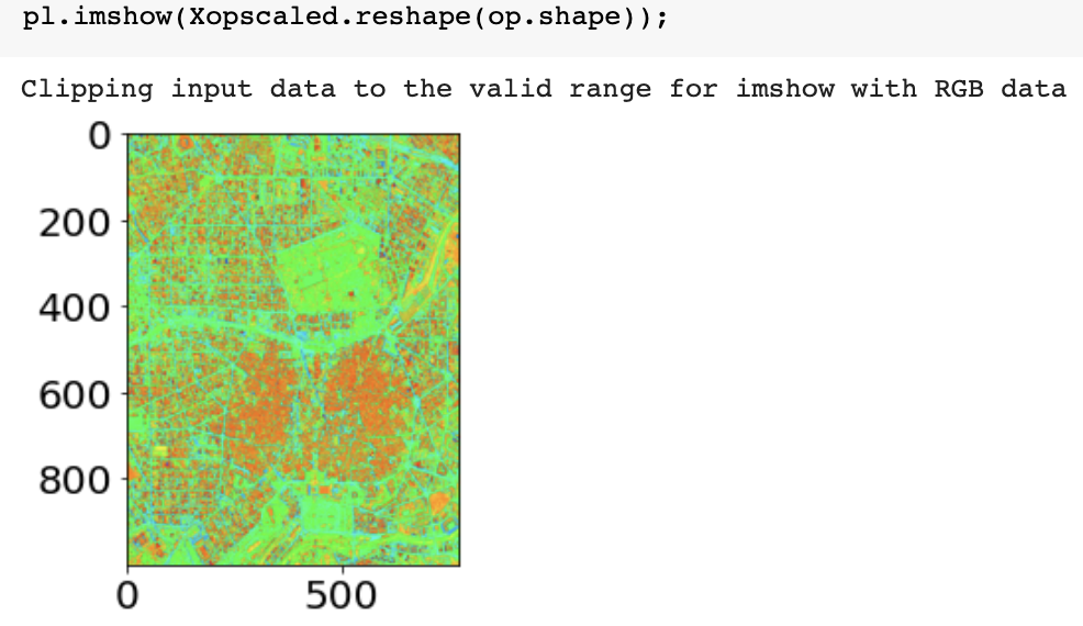
for image processing (e.g. segmentation) often you need to mimmax preprocess
from sklearn import preprocessing
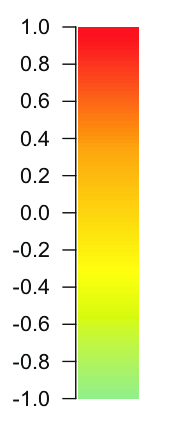
Xopscaled = preprocessing.minmax_scale(image_pixels.astype(float), axis=1)
Xopscaled.reshape(op.shape)[200, 700]before
after (looks the same but colorbar different)
-107
273
0
1
By federica bianco
distances, knn, intro to clustering


