


federica bianco PRO
astro | data science | data for good
dr.federica bianco | fbb.space | fedhere | fedhere
Deep Learning 2 - Convolutional NNs
this slide deck:
Perceptrons are linear classifiers: makes its predictions based on a linear predictor function
combining a set of weights (=parameters) with the feature vector.
.
.
.
output
activation function
weights
bias
output
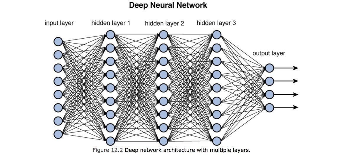
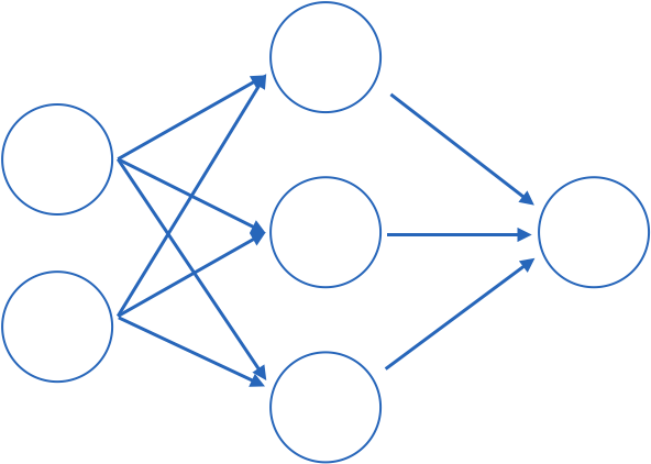
Fully connected: all nodes go to all nodes of the next layer.
input layer
hidden layer
output layer
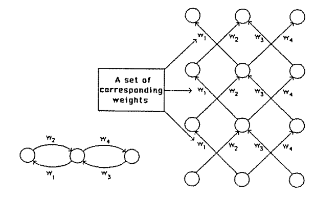
1970: multilayer perceptron architecture
output
layer of perceptrons
output
Fully connected: all nodes go to all nodes of the next layer.
layer of perceptrons
w: weight
sets the sensitivity of a neuron
b: bias:
up-down weights a neuron
learned parameters
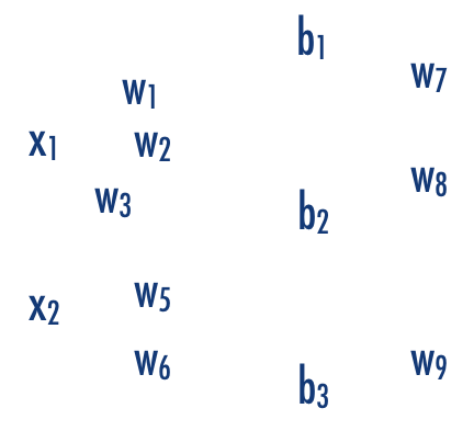
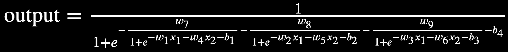
what we are doing is exactly a series of matrix multiplictions.
output
Fully connected: all nodes go to all nodes of the next layer.
layer of perceptrons
w: weight
sets the sensitivity of a neuron
b: bias:
up-down weights a neuron
f: activation function:
turns neurons on-off
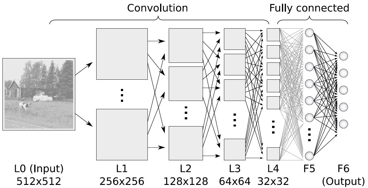
Convolutional Neural Nets
@akumadog
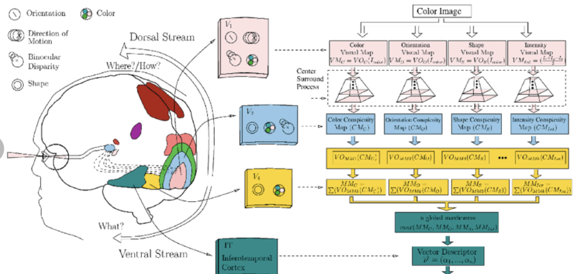
The visual cortex learns hierarchically: first detects simple features, then more complex features and ensembles of features
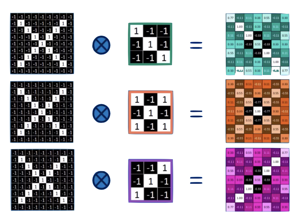
Convolution
Convolution
convolution is a mathematical operator on two functions
f and g
that produces a third function
f x g
expressing how the shape of one is modified by the other.
o
Convolution Theorem
fourier transform
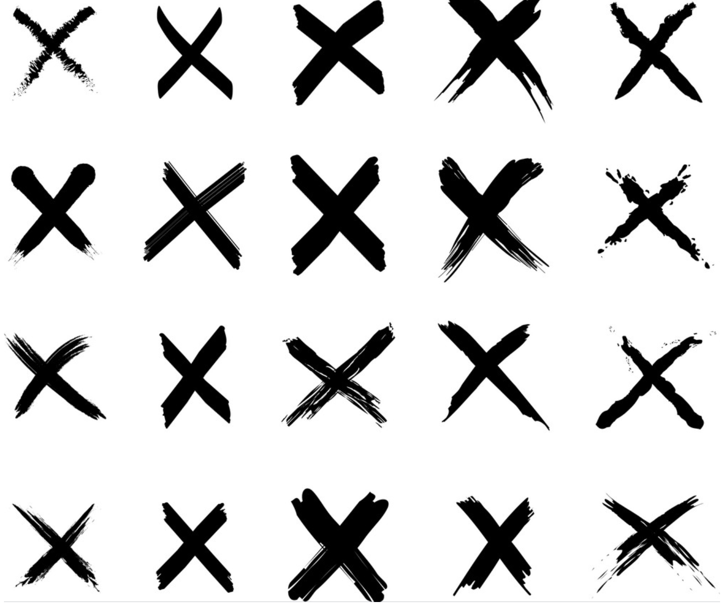
two images.
| -1 | -1 | -1 | -1 | -1 |
|---|---|---|---|---|
| -1 | -1 | -1 | ||
| -1 | -1 | -1 | -1 | |
| -1 | -1 | -1 | ||
| -1 | -1 | -1 | -1 | -1 |
1
1
1
1
1
1
1
1
1
| -1 | -1 | -1 | -1 | -1 |
|---|---|---|---|---|
| -1 | -1 | -1 | -1 | -1 |
| -1 | -1 | -1 | -1 | -1 |
| -1 | -1 | -1 | -1 | -1 |
| -1 | -1 | -1 | -1 | -1 |
| 1 | -1 | -1 |
| -1 | 1 | -1 |
| -1 | -1 | 1 |
1
1
1
1
1
| -1 | -1 | -1 | -1 | -1 |
|---|---|---|---|---|
| -1 | -1 | -1 | ||
| -1 | -1 | -1 | -1 | |
| -1 | -1 | -1 | ||
| -1 | -1 | -1 | -1 | -1 |
| -1 | -1 | 1 |
| -1 | 1 | -1 |
| 1 | -1 | -1 |
feature maps
1
1
1
1
1
convolution
| -1 | -1 | -1 | -1 | -1 |
|---|---|---|---|---|
| -1 | -1 | -1 | ||
| -1 | -1 | -1 | -1 | |
| -1 | -1 | -1 | ||
| -1 | -1 | -1 | -1 | -1 |
| 1 | -1 | -1 |
| -1 | 1 | -1 |
| -1 | -1 | 1 |
1
1
1
1
1
| -1 | -1 | -1 | -1 | -1 |
|---|---|---|---|---|
| -1 | -1 | -1 | ||
| -1 | -1 | -1 | -1 | |
| -1 | -1 | -1 | ||
| -1 | -1 | -1 | -1 | -1 |
| 1 | -1 | -1 |
| -1 | 1 | -1 |
| -1 | -1 | 1 |
| 1 | -1 | -1 |
| -1 | 1 | -1 |
| -1 | -1 | 1 |
| 7 | ||
|---|---|---|
=
1
1
1
1
1
| -1 | -1 | -1 | -1 | -1 |
|---|---|---|---|---|
| -1 | -1 | -1 | ||
| -1 | -1 | -1 | -1 | |
| -1 | -1 | -1 | ||
| -1 | -1 | -1 | -1 | -1 |
| 1 | -1 | -1 |
| -1 | 1 | -1 |
| -1 | -1 | 1 |
| 1 | -1 | -1 |
| -1 | 1 | -1 |
| -1 | -1 | 1 |
| 7 | -3 | |
|---|---|---|
=
1
1
1
1
1
| -1 | -1 | -1 | -1 | -1 |
|---|---|---|---|---|
| -1 | -1 | -1 | ||
| -1 | -1 | -1 | -1 | |
| -1 | -1 | -1 | ||
| -1 | -1 | -1 | -1 | -1 |
| 1 | -1 | -1 |
| -1 | 1 | -1 |
| -1 | -1 | 1 |
| 1 | -1 | -1 |
| -1 | 1 | -1 |
| -1 | -1 | 1 |
| 7 | -3 | 3 |
|---|---|---|
=
1
1
1
1
1
| -1 | -1 | -1 | -1 | -1 |
|---|---|---|---|---|
| -1 | -1 | -1 | ||
| -1 | -1 | -1 | -1 | |
| -1 | -1 | -1 | ||
| -1 | -1 | -1 | -1 | -1 |
| 1 | -1 | -1 |
| -1 | 1 | -1 |
| -1 | -1 | 1 |
| 1 | -1 | -1 |
| -1 | 1 | -1 |
| -1 | -1 | 1 |
| 7 | -3 | 3 |
|---|---|---|
| ? | ||
=
1
1
1
1
1
| -1 | -1 | -1 | -1 | -1 |
|---|---|---|---|---|
| -1 | -1 | -1 | ||
| -1 | -1 | -1 | -1 | |
| -1 | -1 | -1 | ||
| -1 | -1 | -1 | -1 | -1 |
| 1 | -1 | -1 |
| -1 | 1 | -1 |
| -1 | -1 | 1 |
| 1 | -1 | -1 |
| -1 | 1 | -1 |
| -1 | -1 | 1 |
| 7 | -3 | 3 |
|---|---|---|
| ? | ? | |
=
1
1
1
1
1
| -1 | -1 | -1 | -1 | -1 |
|---|---|---|---|---|
| -1 | -1 | -1 | ||
| -1 | -1 | -1 | -1 | |
| -1 | -1 | -1 | ||
| -1 | -1 | -1 | -1 | -1 |
| 1 | -1 | -1 |
| -1 | 1 | -1 |
| -1 | -1 | 1 |
| 1 | -1 | -1 |
| -1 | 1 | -1 |
| -1 | -1 | 1 |
| 7 | -3 | 3 |
|---|---|---|
| ? | ? | |
=
1
1
1
1
1
| -1 | -1 | -1 | -1 | -1 |
|---|---|---|---|---|
| -1 | -1 | -1 | ||
| -1 | -1 | -1 | -1 | |
| -1 | -1 | -1 | ||
| -1 | -1 | -1 | -1 | -1 |
| 1 | -1 | -1 |
| -1 | 1 | -1 |
| -1 | -1 | 1 |
| 1 | -1 | -1 |
| -1 | 1 | -1 |
| -1 | -1 | 1 |
| 7 | -3 | 3 |
|---|---|---|
| ? | ? | |
=
1
1
1
1
1
| -1 | -1 | -1 | -1 | -1 |
|---|---|---|---|---|
| -1 | -1 | -1 | ||
| -1 | -1 | -1 | -1 | |
| -1 | -1 | -1 | ||
| -1 | -1 | -1 | -1 | -1 |
| 1 | -1 | -1 |
| -1 | 1 | -1 |
| -1 | -1 | 1 |
| 1 | -1 | -1 |
| -1 | 1 | -1 |
| -1 | -1 | 1 |
| 7 | -3 | 3 |
|---|---|---|
| ? | ? | |
=
1
1
1
1
1
| -1 | -1 | -1 | -1 | -1 |
|---|---|---|---|---|
| -1 | -1 | -1 | ||
| -1 | -1 | -1 | -1 | |
| -1 | -1 | -1 | ||
| -1 | -1 | -1 | -1 | -1 |
| 1 | -1 | -1 |
| -1 | 1 | -1 |
| -1 | -1 | 1 |
| 1 | -1 | -1 |
| -1 | 1 | -1 |
| -1 | -1 | 1 |
| 7 | -3 | 3 |
|---|---|---|
| ? | ? | |
=
1
1
1
1
1
| -1 | -1 | -1 | -1 | -1 |
|---|---|---|---|---|
| -1 | -1 | -1 | ||
| -1 | -1 | -1 | -1 | |
| -1 | -1 | -1 | ||
| -1 | -1 | -1 | -1 | -1 |
| 1 | -1 | -1 |
| -1 | 1 | -1 |
| -1 | -1 | 1 |
| 7 | -3 | 3 |
|---|---|---|
| -3 | ||
=
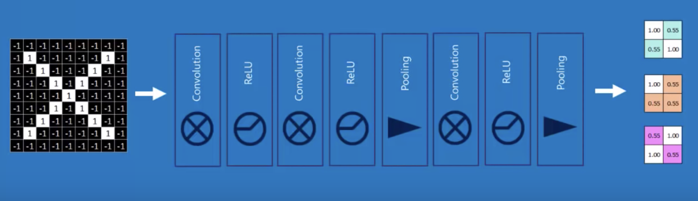
input layer
feature map
convolution layer
1
1
1
1
1
| -1 | -1 | -1 | -1 | -1 |
|---|---|---|---|---|
| -1 | -1 | -1 | ||
| -1 | -1 | -1 | -1 | |
| -1 | -1 | -1 | ||
| -1 | -1 | -1 | -1 | -1 |
| 1 | -1 | -1 |
| -1 | 1 | -1 |
| -1 | -1 | 1 |
| 7 | -3 | 3 |
| -3 | 5 | -3 |
| 3 | -3 | 7 |
=
input layer
feature map
convolution layer
the feature map is "richer": we went from binary to R
1
1
1
1
1
| -1 | -1 | -1 | -1 | -1 |
|---|---|---|---|---|
| -1 | -1 | -1 | ||
| -1 | -1 | -1 | -1 | |
| -1 | -1 | -1 | ||
| -1 | -1 | -1 | -1 | -1 |
| 1 | -1 | -1 |
| -1 | 1 | -1 |
| -1 | -1 | 1 |
=
input layer
feature map
convolution layer
the feature map is "richer": we went from binary to R
and it is reminiscent of the original layer
7
5
7
| 7 | -3 | 3 |
| -3 | 5 | -3 |
| 3 | -3 | 7 |
=
7
7
Convolve with different feature: each neuron is 1 feature
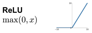
ReLu
| 7 | -3 | 3 |
| -5 | 5 | -3 |
| -6 | -1 | 7 |
7
5
7
ReLu: normalization that replaces negative values with 0's
| 7 | 0 | 3 |
| 0 | 5 | 0 |
| 3 | 0 | 7 |
7
5
7
Max-Pool
MaxPooling: reduce image size, generalizes result
| 7 | 0 | 3 |
| 0 | 5 | 0 |
| 3 | 0 | 7 |
7
5
7
MaxPooling: reduce image size, generalizes result
| 7 | 0 | 3 |
| 0 | 5 | 0 |
| 3 | 0 | 7 |
7
5
7
2x2 Max Poll
| 7 | 5 |
MaxPooling: reduce image size, generalizes result
| 7 | 0 | 3 |
| 0 | 5 | 0 |
| 3 | 0 | 7 |
7
5
7
2x2 Max Poll
| 7 | 5 |
| 5 |
MaxPooling: reduce image size, generalizes result
| 7 | 0 | 3 |
| 0 | 5 | 0 |
| 3 | 0 | 7 |
7
5
7
2x2 Max Poll
| 7 | 5 |
| 5 | 7 |
MaxPooling: reduce image size & generalizes result
By reducing the size and picking the maximum of a sub-region we make the network less sensitive to specific details
x
O
last hidden layer
output layer
Stack multiple convolution layers
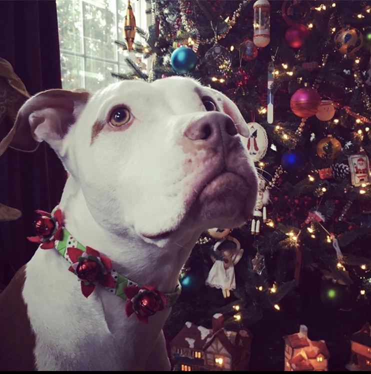
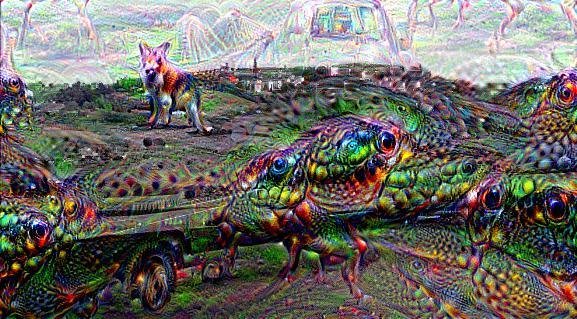
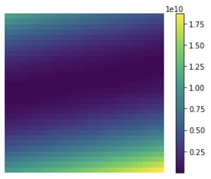
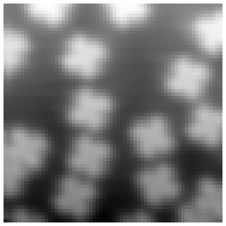
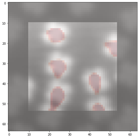
Deep Dream (DD) is a google software, a pre-trained NN (originally created on the Cafe architecture, now imported on many other platforms including tensorflow).
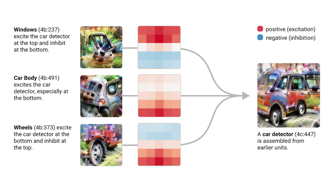
The high level idea relies on training a convolutional NN to recognize common objects, e.g. dogs, cats, cars, in images. As the network learns to recognize those objects is develops its convolutional layers to pick out "features" of the NN, like lines at a certain orientations, circles, etc.
Each neuron, is a filters: e.g. edge finders.
The DeepDream software runs this NN on an image you give it, and it loops on some hidden layers, thus "manifesting" the things it knows how to recognize in the image. The output of an inner layer (input of the next inner layer) is called a "feature map". We are taking a peek into the feature maps of a deep neural network trained to recognized common onbjects.
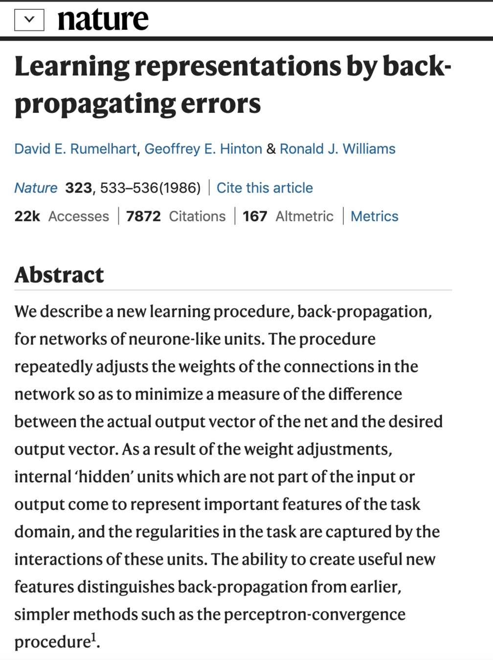
Deep Learning
excellent blog post on BP: http://colah.github.io/posts/2015-08-Backprop/
First, compute the linear function for state of neuron,
First, compute the linear function for state of neuron,
x
y
First, compute the linear function for state of neuron,
x
y
minimize L2 by changing w iteratively
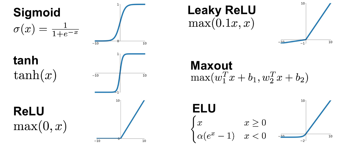
Then, calculate the output of that layer by using a non-linear function.
x
y
activation
function
(Sigmoid)
to perform classification
Then, calculate the output of that layer by using non-linear function.
.
.
.
sigmoid
output
.
.
.
Any linear model:
y : prediction
ytrue : target
Error: e.g.
intercept
slope
L2
x
Find the best parameters by finding the minimum of the L2 hyperplane
at every step look around and choose the best direction
how does linear descent look when you have a whole network structure with hundreds of weights and biases to optimize??
.
.
.
output
f: activation function:
turns neurons on-off
w: weight
sets the sensitivity of a neuron
b: bias:
up-down weights a neuron
In a CNN these layers would not be fully connected except the last one
.
.
.
perceptron or
shallow NN
input layer
hidden layer
output layer
Training models with this many parameters requires a lot of care:
. defining the metric
. optimization schemes
. training/validation/testing sets
But just like our simple linear regression case, the fact that small changes in the parameters leads to small changes in the output for the right activation functions.
define a cost function, e.g.
Training a DNN
feed data forward through network and calculate cost metric
for each layer, calculate effect of small changes on next layer
how does linear descent look when you have a whole network structure with hundreds of weights and biases to optimize??
think of applying just gradient to a function of a function of a function... use:
1) partial derivatives, 2) chain rule
define a cost function, e.g.
Training a DNN
Minibatch
&
Dropout
Split your training set into many smaller subsets and train on each small set separately
Dropout
Artificially remove some neurons for different minibatches to avoid overfitting
output
Architecture components: neurons, activation function
Single layer NN: perceptrons
Deep NN:
Convolutional NN
Training an NN:
Lots of parameters and lots of hyperparameters! What to choose?
cheatsheet
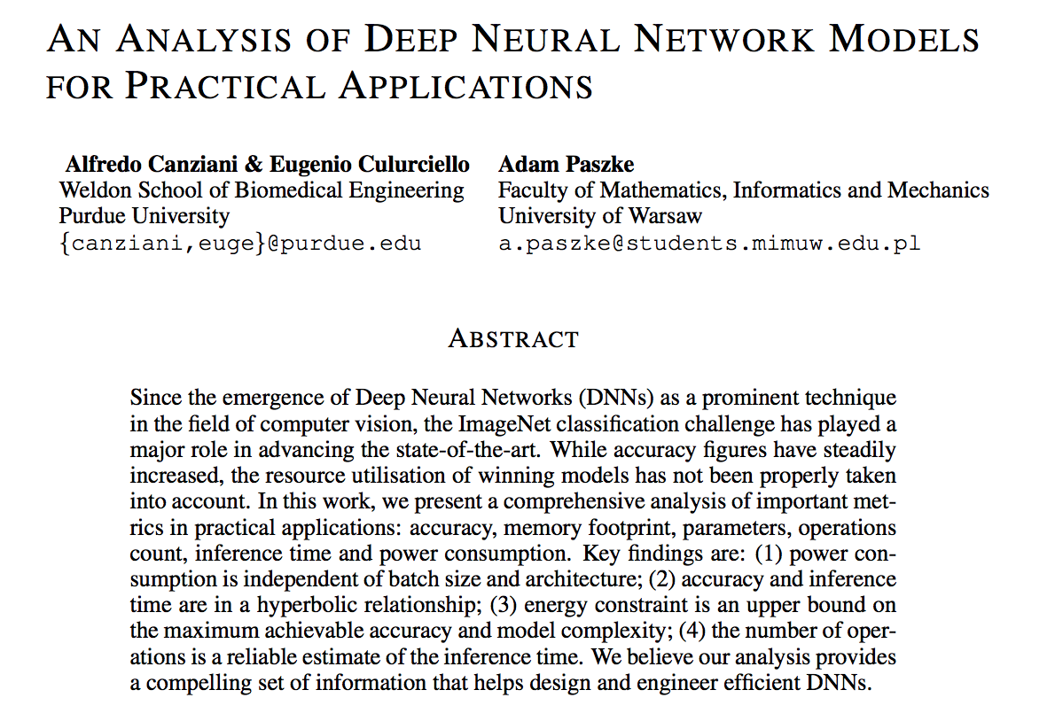
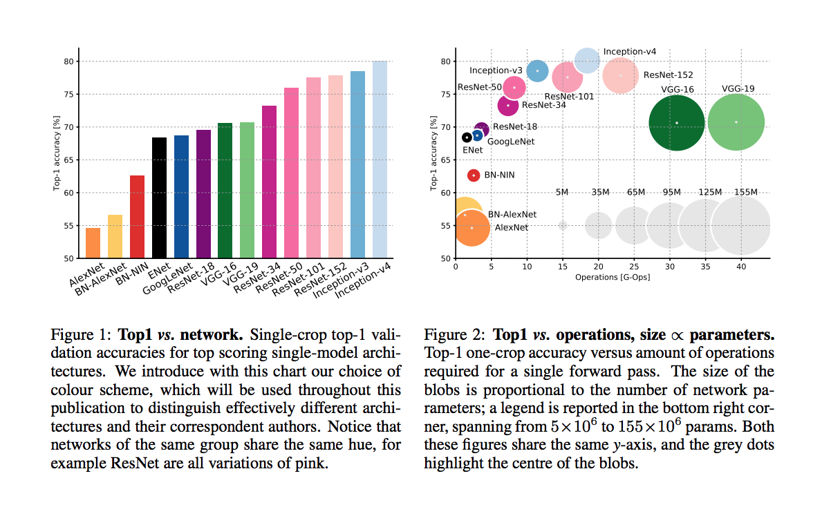
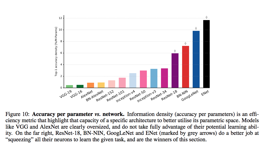
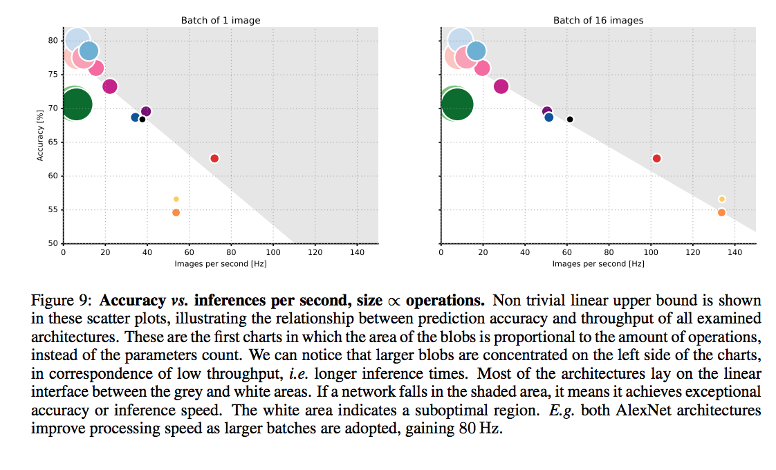
An article that compars various DNNs
An article that compars various DNNs
accuracy comparison
An article that compars various DNNs
accuracy comparison
An article that compars various DNNs
batch size
Lots of parameters and lots of hyperparameters! What to choose?
cheatsheet
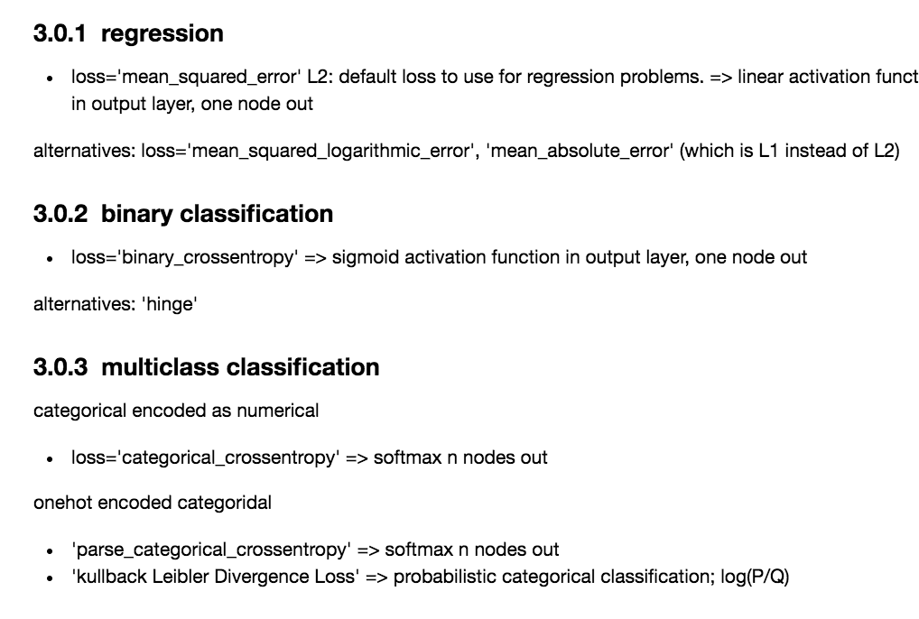
What should I choose for the loss function and how does that relate to the activation functiom and optimization?
Lots of parameters and lots of hyperparameters! What to choose?
Lots of parameters and lots of hyperparameters! What to choose?
cheatsheet
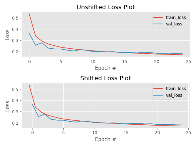
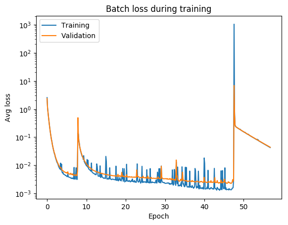
always check your loss function! it should go down smoothly and flatten out at the end of the training.
not flat? you are still learning!
too flat? you are overfitting...
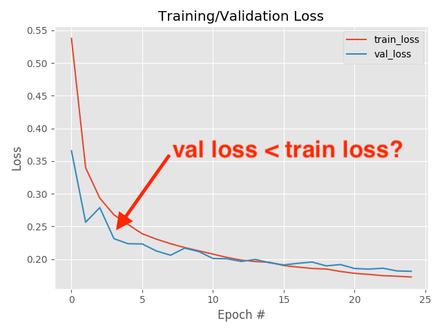
loss (gallery of horrors)
jumps are not unlikely (and not necessarily a problem) if your activations are discontinuous (e.g. relu)
when you use validation you are introducing regularizations (e.g. dropout) so the loss can be smaller than for the training set
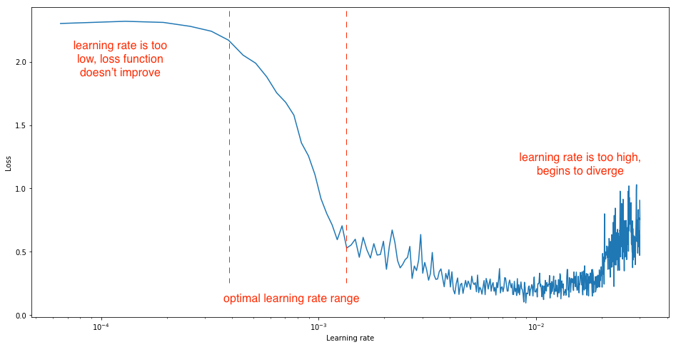
loss and learning rate (not that the appropriate learning rate depends on the chosen optimization scheme!)
Building a DNN
with keras and tensorflow
autoencoder for image recontstruction
What should I choose for the loss function and how does that relate to the activation functiom and optimization?
| loss | good for | activation last layer | size last layer |
|---|---|---|---|
| mean_squared_error | regression | linear | one node |
| mean_absolute_error | regression | linear | one node |
| mean_squared_logarithmit_error | regression | linear | one node |
| binary_crossentropy | binary classification | sigmoid | one node |
| categorical_crossentropy | multiclass classification | sigmoid | N nodes |
| Kullback_Divergence | multiclass classification, probabilistic inerpretation | sigmoid | N nodes |
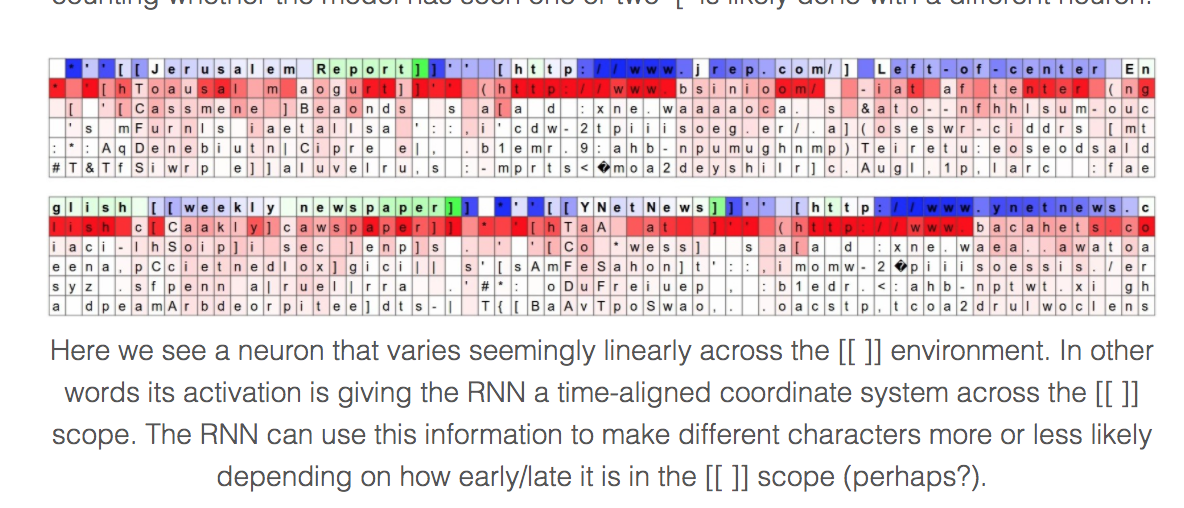
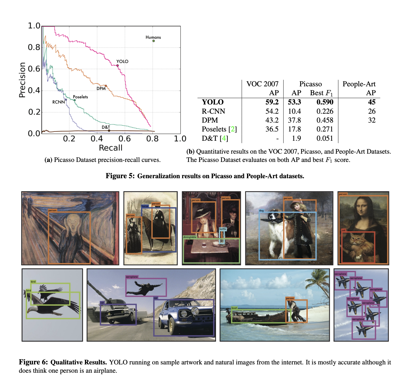
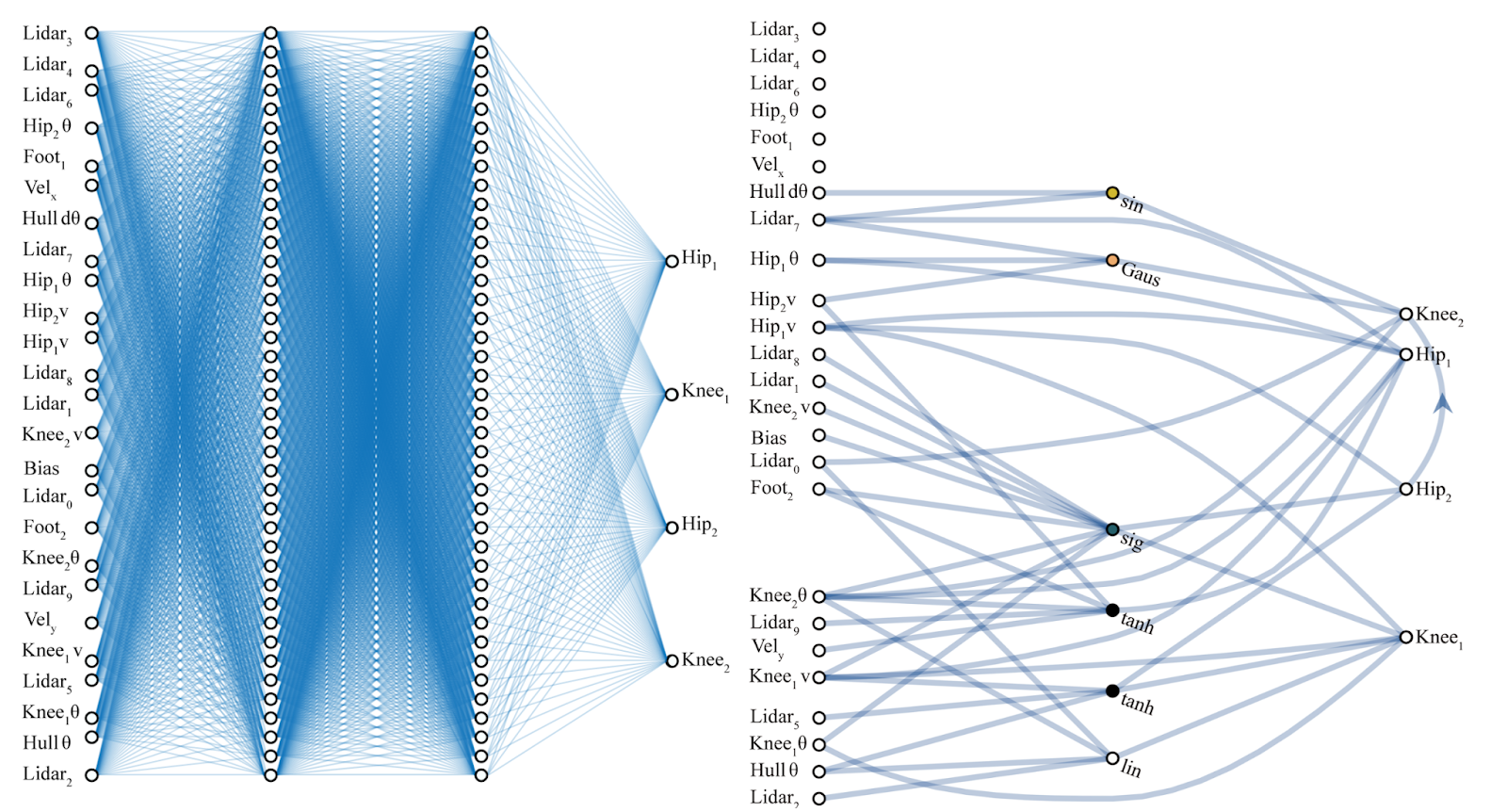
On the interpretability of DNNs
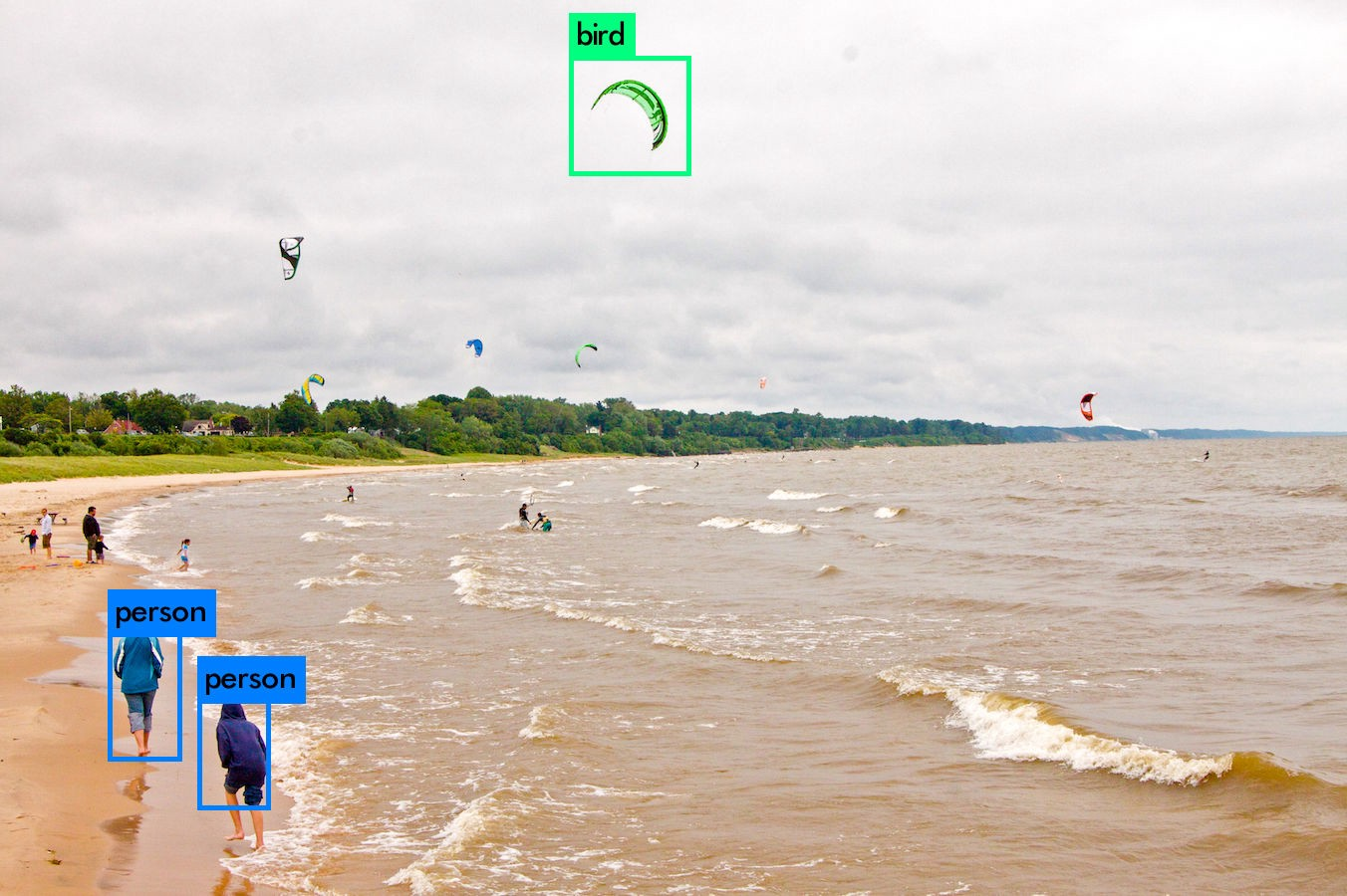
YOLO and R-CNN
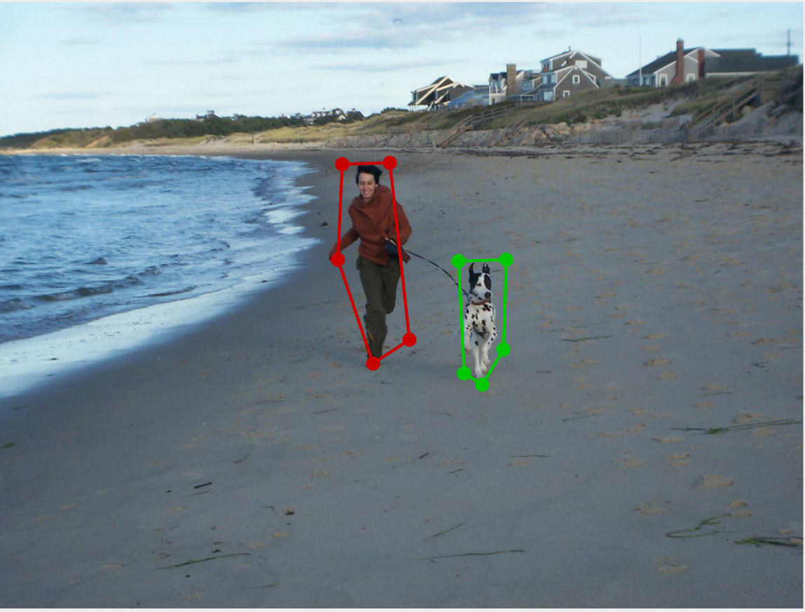
Object detection
Naive model: we took different region of the image and measured the probability of presence of the object in that region
YOLO and R-CNN
Object detection
Problem: we had to search the whole image which is time consuming, we could only find 1 kind of object at 1 scale
YOLO and R-CNN
Object detection
Problem: we had to search the whole image which is time consuming, we could only find 1 kind of object at 1 scale
YOLO and R-CNN
Object detection
What if you do not know what is in the mage?
Final Dense layer has undefined size (one per kind of object in the region)
Objects can have different scale or axis ration: how many regions can you search before the problem blows up computationally??
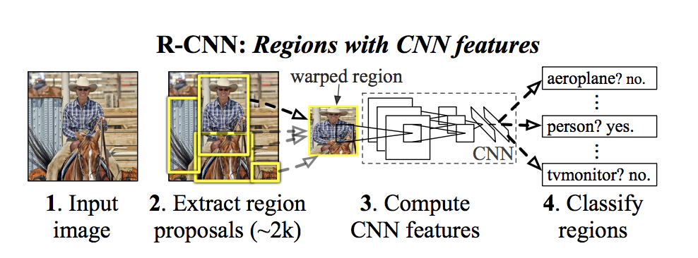
R-CNN
Extract 2000 regions from the image "region proposals."
Feature Extraction CNN produces a 4096-dimensional feature vector in an output dense layer
SVM classify the presence of the object within that candidate region proposal.
1. Generate initial sub-segmentation, we generate many candidate     regions
2. Use greedy algorithm to recursively combine similar regions into larger ones
3. Use the generated regions to produce the final candidate region proposals
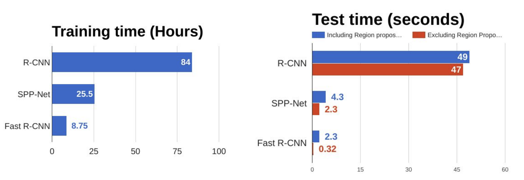
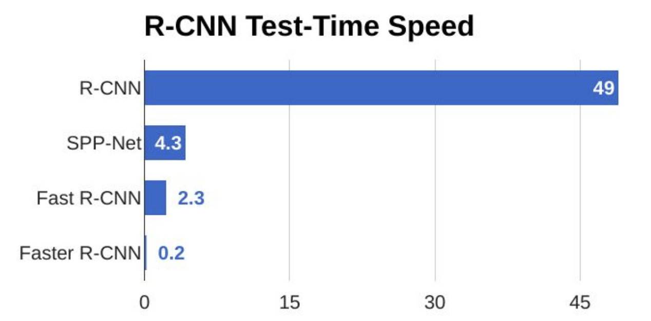
TOO SLOW (47 sec to test 1 image)
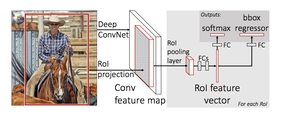
Fast R-CNN
Use a CNN to generate convolutional feature maps
Use Selective Search Algorithm to tdentify the RPs and warp them into squares
Using an RoI pooling layer to reshape them into a fixed size so that it can be fed into a fully connected layer - predict box offset
Softmax layer to predict the class of the proposed
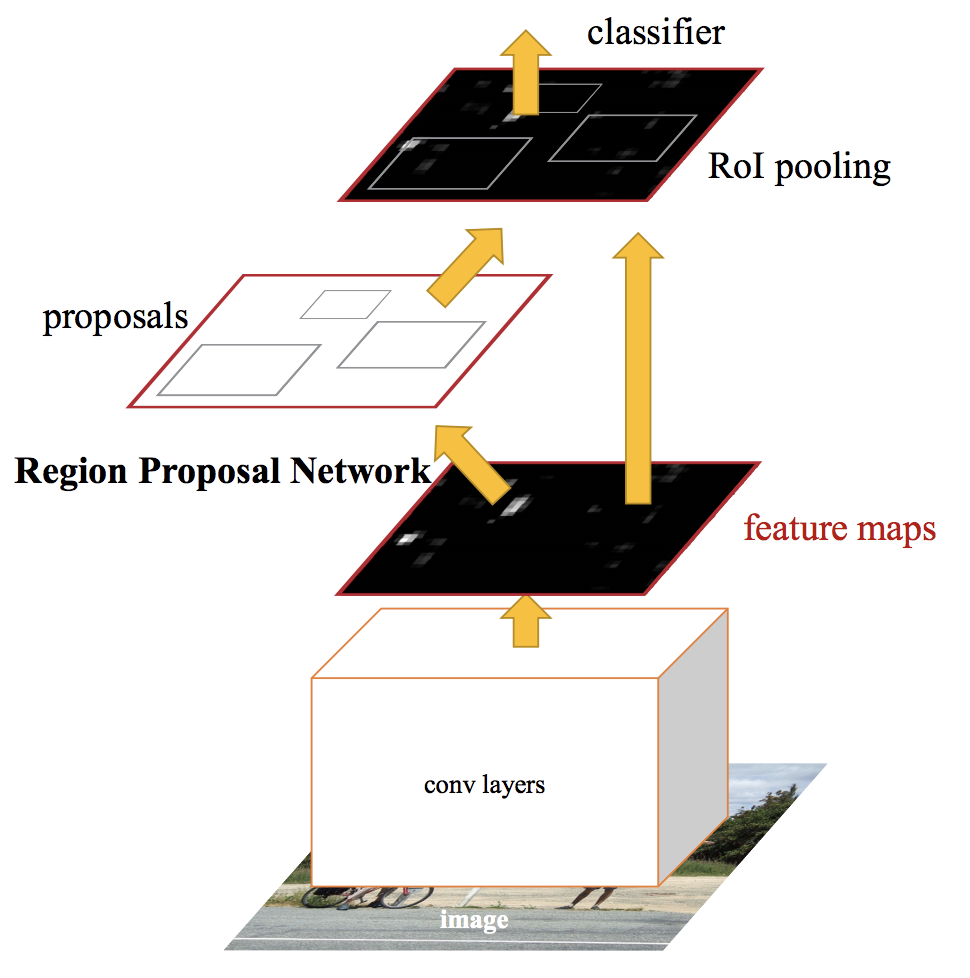
Faster R-CNN
Use a CNN to generate convolutional feature maps
Use CNN to predict RPs and warp them into squares
Using an RoI pooling layer to reshape them into a fixed size so that it can be fed into a fully connected layer - predict box offset
Softmax layer to predict the class of the proposed
Faster R-CNN
Ren et al. 2015
Use a CNN to generate convolutional feature maps
Use CNN to predict RPs and warp them into squares
Using an RoI pooling layer to reshape them into a fixed size so that it can be fed into a fully connected layer - predict box offset
Softmax layer to predict the class of the proposed
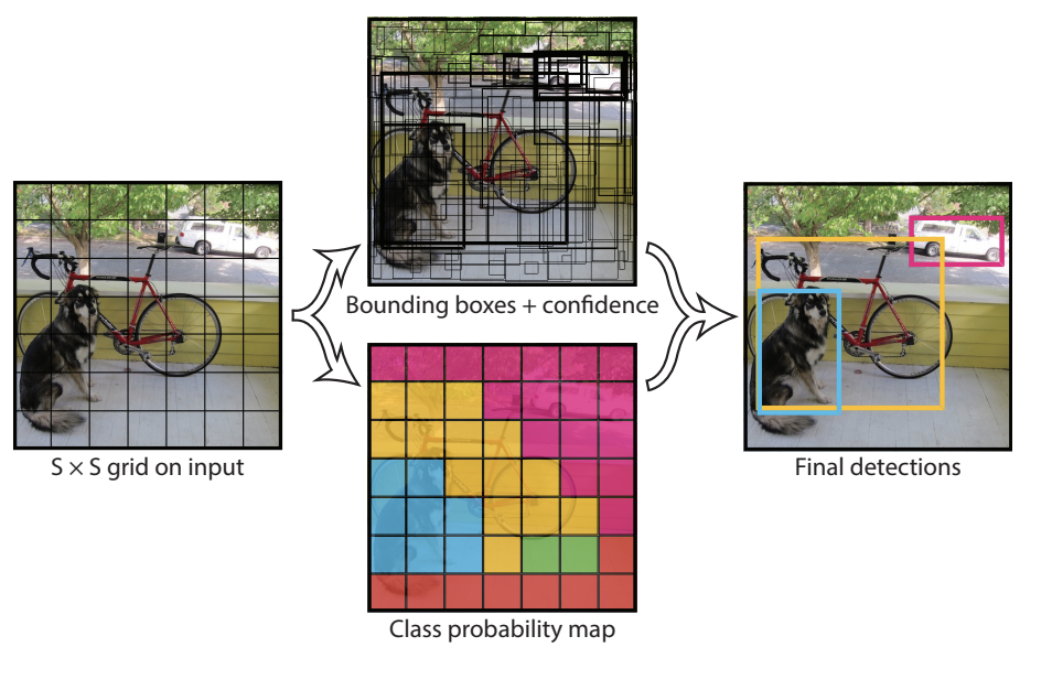
Yolo
What if you looked at the whole image instead of RoIs in the image??
Split an image into a SxS grid
For each grid cell predicts B bounding boxes, confidence for those boxes, and C class probabilities.
CNN outputs probability that BB has an object (+ offset)
High prob BBs are classified
Labling tools
Neural Network and Deep Learning
an excellent and free book on NN and DL
http://neuralnetworksanddeeplearning.com/index.html
History of NN
https://cs.stanford.edu/people/eroberts/courses/soco/projects/neural-networks/History/history2.html
Gradient Descent
https://ml-cheatsheet.readthedocs.io/en/latest/gradient_descent.html
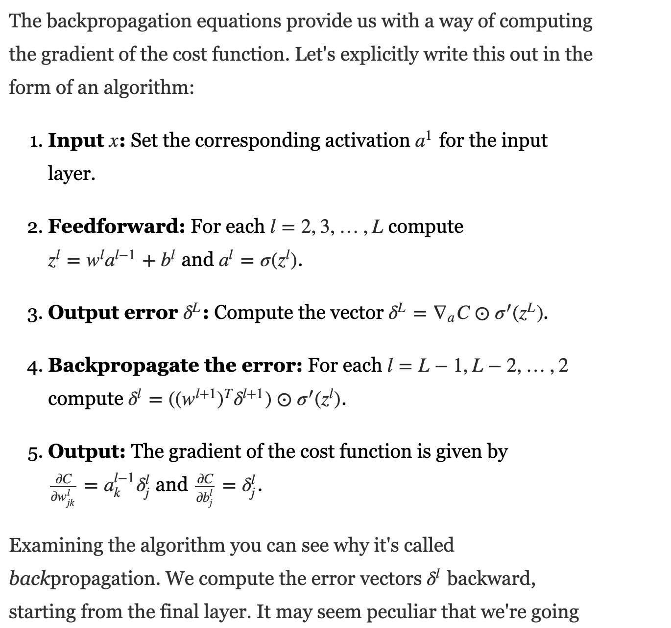
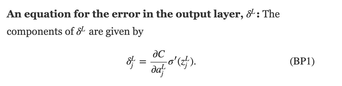
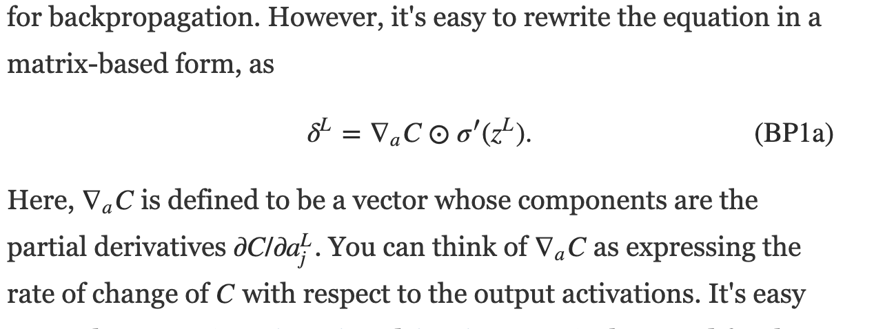
Backpropagation
http://colah.github.io/posts/2015-08-Backprop/
Physics Informed NN
Application regime:
-infinity - 1950's
theory driven: little data, mostly theory, falsifiability and all that...
Application regime:
-infinity - 1950's
theory driven: little data, mostly theory, falsifiability and all that...
-1980's - today
data driven: lots of data, drop theory and use associations, black-box modles
Application regime:
-infinity - 1950's
theory driven: little data, mostly theory, falsifiability and all that...
-1980's - today
data driven: lots of data, drop theory and use associations, black-box modles
lots of data yet not enough for entirely automated decision making
complex theory that cannot be solved analytically
combine it with some theory
General conservation law
e.g. flux function (linear)
Burgers eq (non-linear)
is a nonlinear differential operator
Non Linear PDEs are hard to solve!
A fundamental question for any PDE is the existence and uniqueness of a solution for given boundary conditions. open problem of existence (and smoothness) of solutions to the Navier–Stokes equations is one of the seven Millennium Prize problems in mathematics.
Non Linear PDEs are hard to solve!
The solutions in a neighborhood of a known solution can sometimes be studied by linearizing the PDE around the solution. This corresponds to studying the tangent space of a point of the moduli space of all solutions.
Non Linear PDEs are hard to solve!
It is often possible to write down some special solutions explicitly in terms of elementary functions (though it is rarely possible to describe all solutions like this). One way of finding such explicit solutions is to reduce the equations to equations of lower dimension, preferably ordinary differential equations, which can often be solved exactly.
Non Linear PDEs are hard to solve!
Numerical solution on a computer is almost the only method that can be used for getting information about arbitrary systems of PDEs. There has been a lot of work done, but a lot of work still remains on solving certain systems numerically, especially for the Navier–Stokes and other equations related to weather prediction.
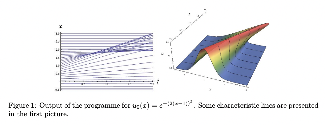
Burgers equation:
second order non-linear PDE
spatial coordinate
temporal coordinate
speef of fluid at x,t
viscosity
Applications of Burgers eq:
shock weave formation, turbulence, the weather problem, traffic flow and acoustic transmission
Domain
Boundary Conditions
How to solve analytically
https://www.youtube.com/watch?v=5ZrwxQr6aV4
Burgers equation:
second order non-linear PDE
How to solve analytically
https://www.youtube.com/watch?v=5ZrwxQr6aV4
Burgers equation:
second order non-linear PDE
input layer
???
via a modified loss function that includes residuals of the prediction and residual of the PDE
via a modified loss function that includes residuals of the prediction and residual of the PDE
via a modified loss function that includes residuals of the prediction and residual of the PDE
By federica bianco
convolutinl NN


