


federica bianco PRO
astro | data science | data for good
Linear Regression and Decomposition
Spring 2025 - UDel PHYS 664
dr. federica bianco
@fedhere
this slide deck:
python github google-colab stackoverflow
1
Reproducible research means:
all numbers in a data analysis can be recalculated exactly (down to stochastic variables!) using the code and raw data provided by the analyst.
Claerbout, J. 1990,
Active Documents and Reproducible Results, Stanford Exploration Project Report, 67, 139
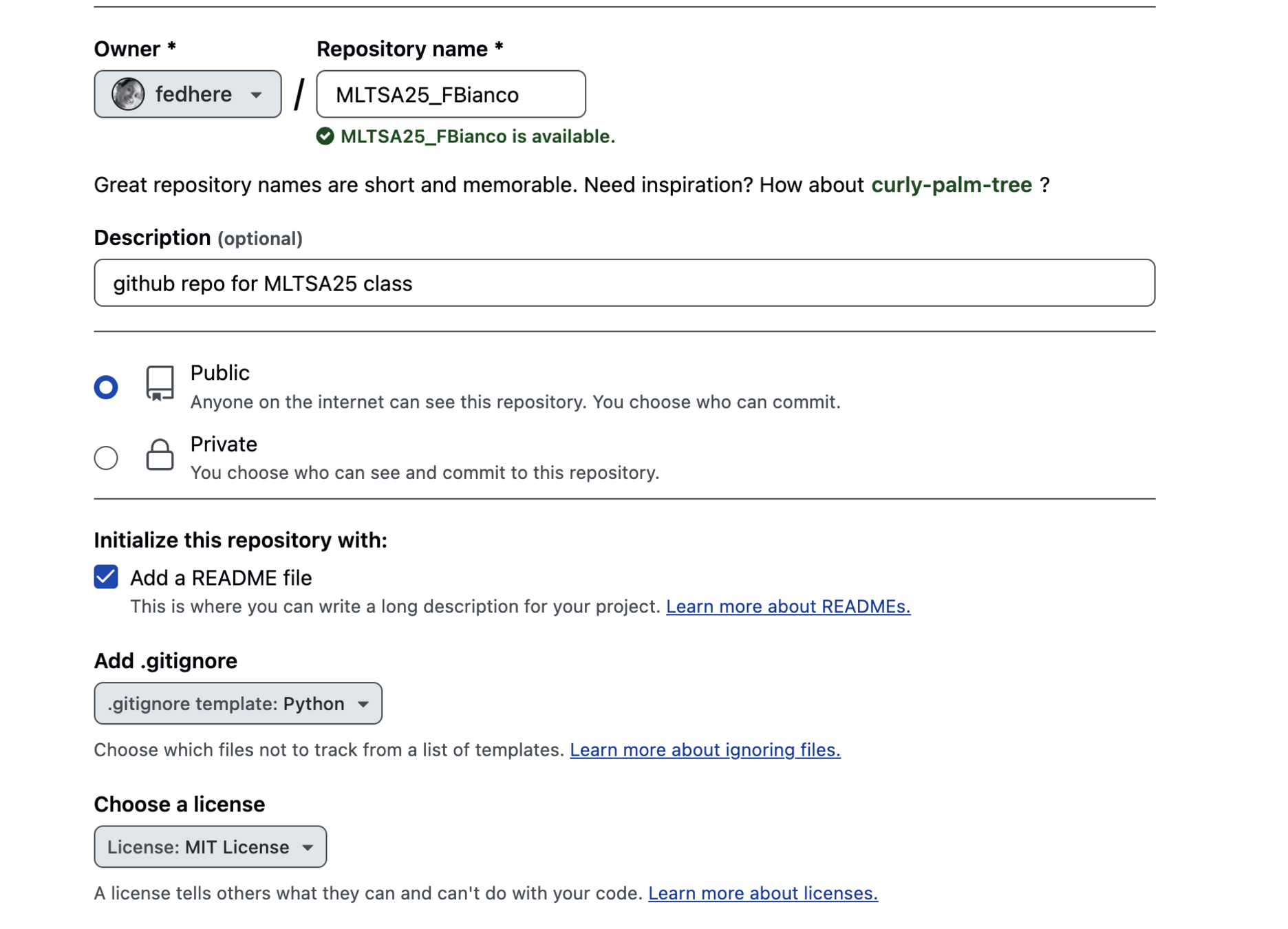
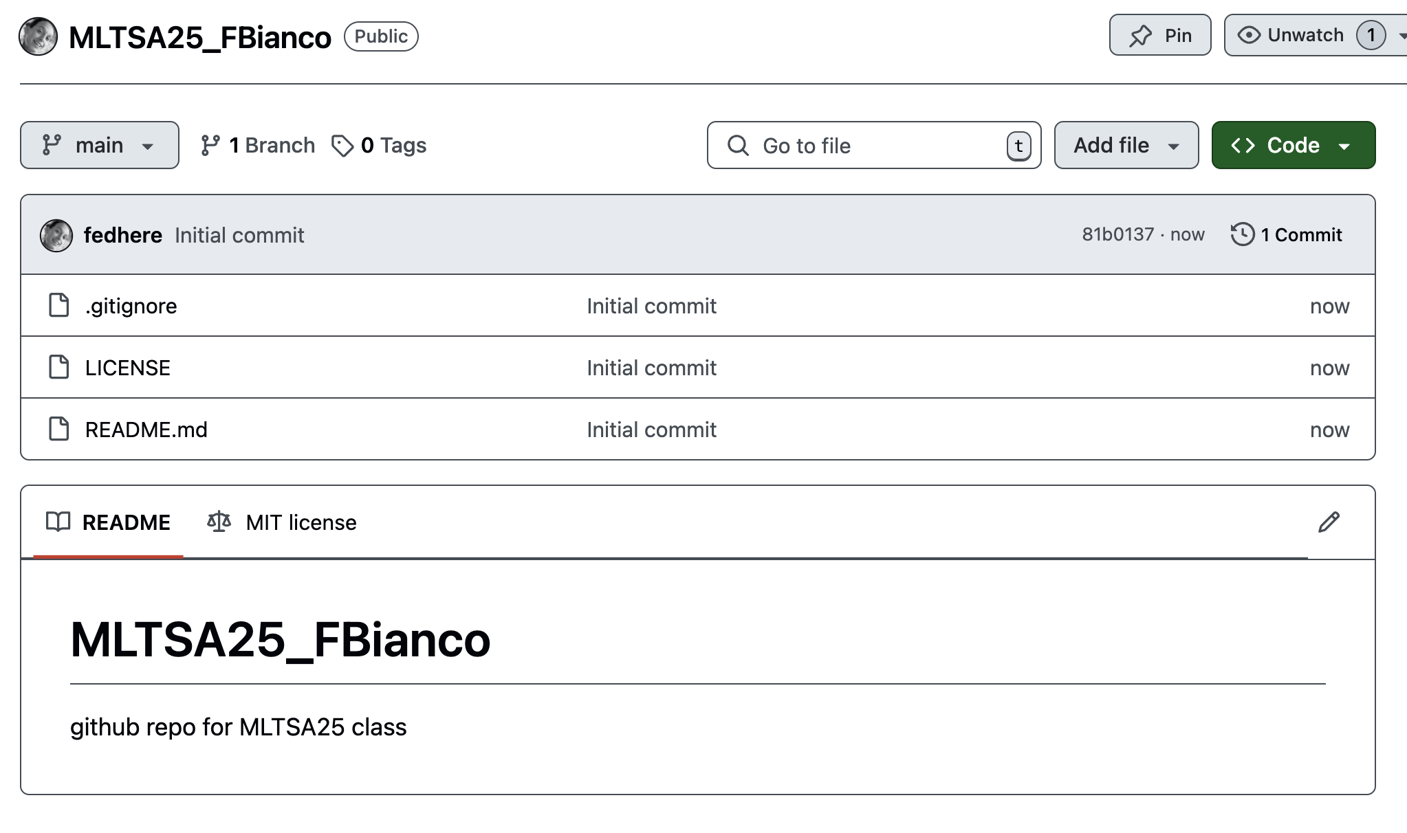
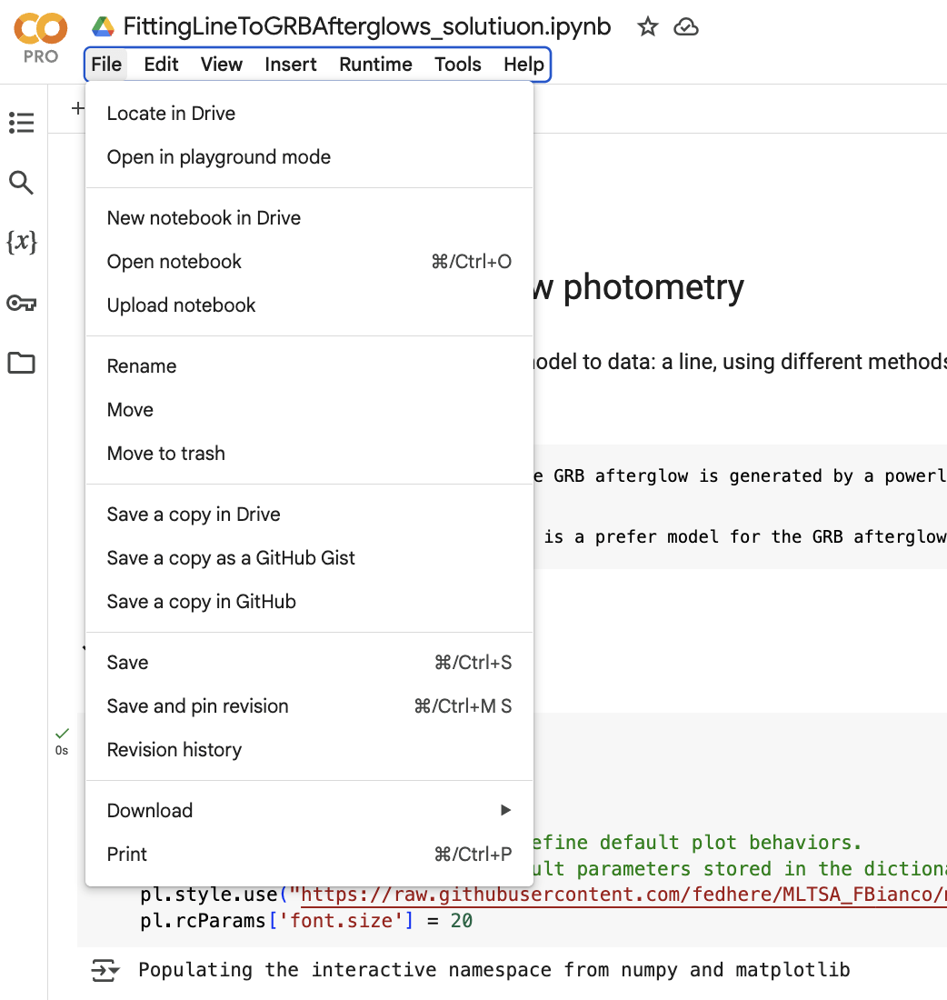
allows reproducibility through code distribution
the Git software
is a distributed version control system:
a version of the files on your local computer is made also available at a central server.
The history of the files is saved remotely so that any version (that was checked in) is retrievable.
allows version control
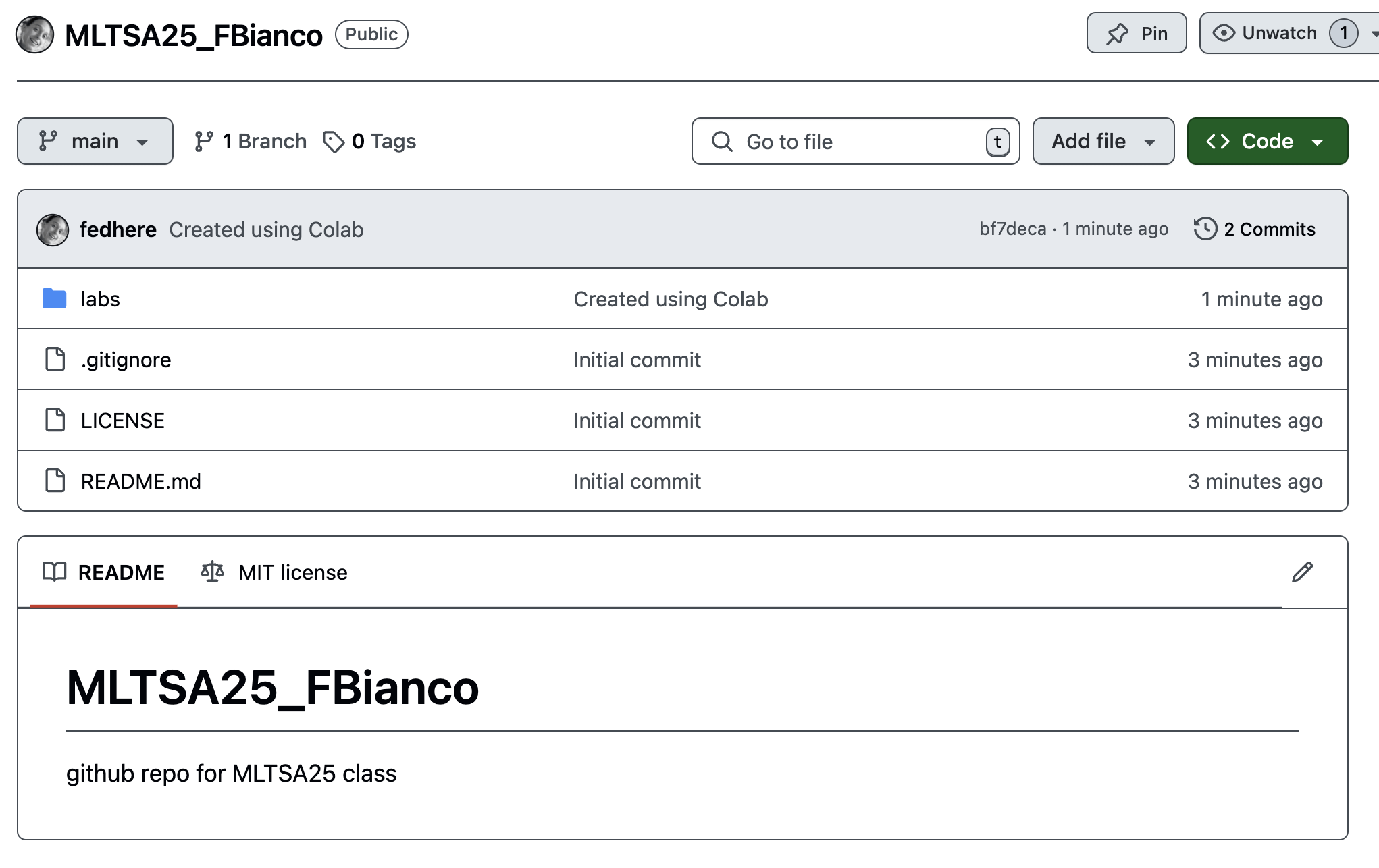
collaboration tool
by fork, fork and pull request, or by working directly as a collaborator
allows effective collaboration
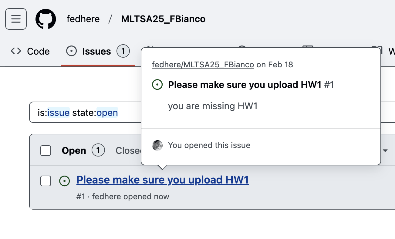
If something is wrong with your repo I will communicate that with an Issue - please attend to your issues promptly
Science Guiding Principles
2
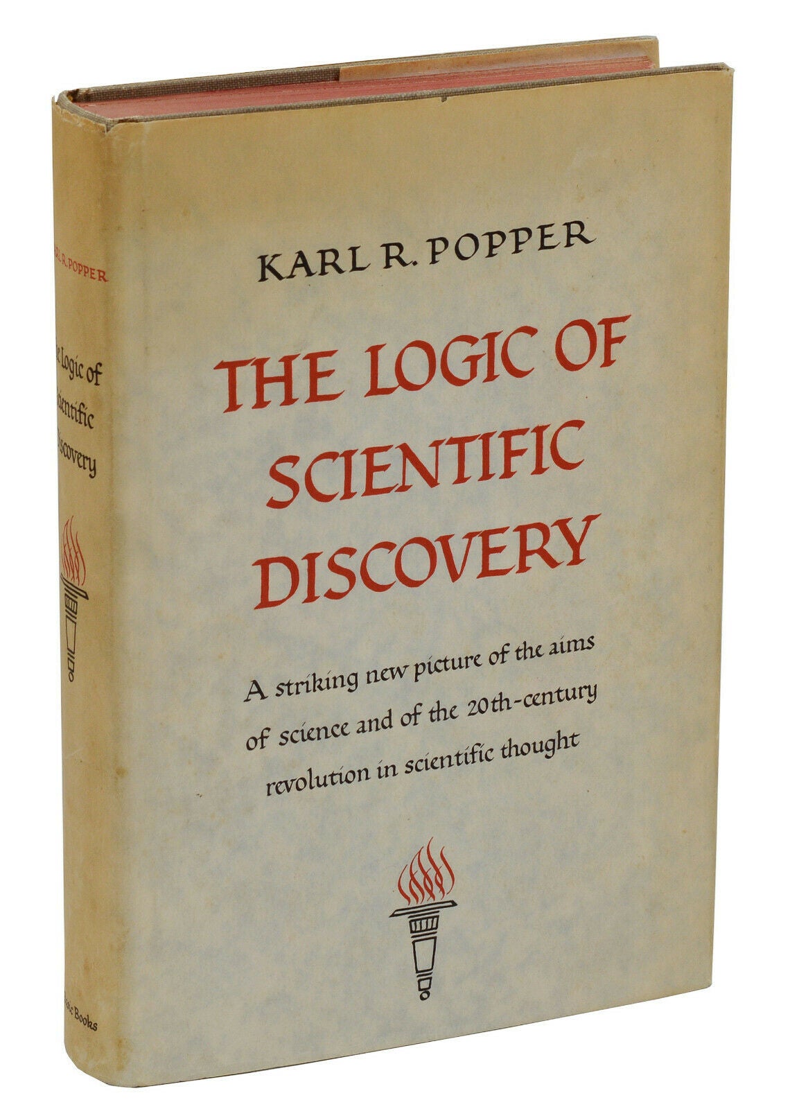
My proposal is based upon an asymmetry between verifiability and falsifiability; an asymmetry which results from the logical form of universal statements. For these are never derivable from singular statements, but can be contradicted by singular statements.
—Karl Popper, The Logic of Scientific Discovery
the demarcation problem:
what is science? what is not?
a scientific theory must be falsifiable
My proposal is based upon an asymmetry between verifiability and falsifiability; an asymmetry which results from the logical form of universal statements. For these are never derivable from singular statements, but can be contradicted by singular statements.
—Karl Popper, The Logic of Scientific Discovery
the demarcation problem:
what is science? what is not?
model
prediction
the demarcation problem
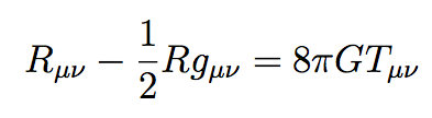
Einstein GR
the demarcation problem
model
prediction
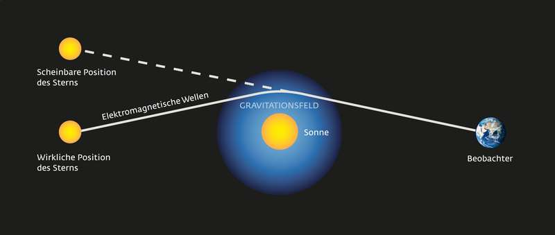
Light rays are deflected by mass
model
prediction
data
does not falsify
falsifies
GR
still holds
GR
rejected
the demarcation problem
position of star changes during eclipse
position of star does not change during eclipse
is astrology a science?
the demarcation problem
DISCUSS!
the demarcation problem
things can get more complicated though:
most scientific theories are actually based largely on probabilistic induction and
modern inductive inference (Solomonoff, frequentist vs Bayesian methods...)
the demarcation problem
A theory can be said to be scientific if it makes falsifiable predictions
Experiments should be designed to falsify the predictions
Key Concept
Reproducible research means:
the ability of a researcher to duplicate the results of a prior study using the same materials as were used by the original investigator. That is, a second researcher might use the same raw data to build the same analysis files and implement the same statistical analysis in an attempt to yield the same results.
assures a result is grounded in evidence
1
#openscience
#opendata
Reproducible research means:
the ability of a researcher to duplicate the results of a prior study using the same materials as were used by the original investigator. That is, a second researcher might use the same raw data to build the same analysis files and implement the same statistical analysis in an attempt to yield the same results.
facilitates scientific progress by avoiding the need to duplicate unoriginal research
2
Reproducible research means:
the ability of a researcher to duplicate the results of a prior study using the same materials as were used by the original investigator. That is, a second researcher might use the same raw data to build the same analysis files and implement the same statistical analysis in an attempt to yield the same results.
facilitate collaboration and teamwork
3
Reproducible research in practice:
using the code and raw data provided by the analyst.
Claerbout, J. 1990,
Active Documents and Reproducible Results, Stanford Exploration Project Report, 67, 139
Reproducible research means:
the ability of a researcher to duplicate the results of a prior study using the same materials as were used by the original investigator. That is, a second researcher might use the same raw data to build the same analysis files and implement the same statistical analysis in an attempt to yield the same results.
all numbers in a data analysis can be recalculated exactly (down to stochastic variables!)
Reproducible research means:
the ability of a researcher to duplicate the results of a prior study using the same materials as were used by the original investigator. That is, a second researcher might use the same raw data to build the same analysis files and implement the same statistical analysis in an attempt to yield the same results.
Reproducible research in practice:
using the code and raw data provided by the analyst.
all numbers in a data analysis can be recalculated exactly (down to stochastic variables!)
A research product is reproducible if all numbers can be reproduced exactly be applying the same code to the same raw data.
It is the responsibility of the researcher to provide the data and code that make a research product reproducible
Key Concept
Recap
3
Linear Regression
WHY?
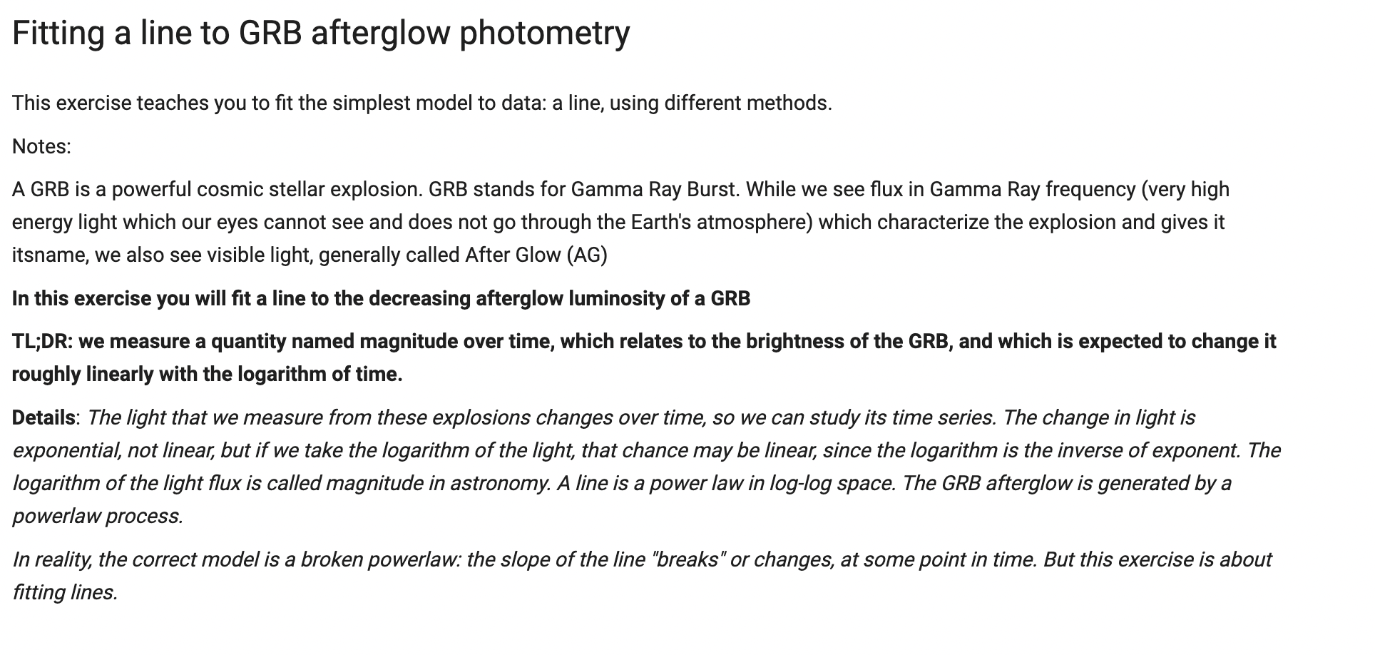
Fitting a line
ax+b
to data y
WHY?
Fitting a line
ax+b
to data y
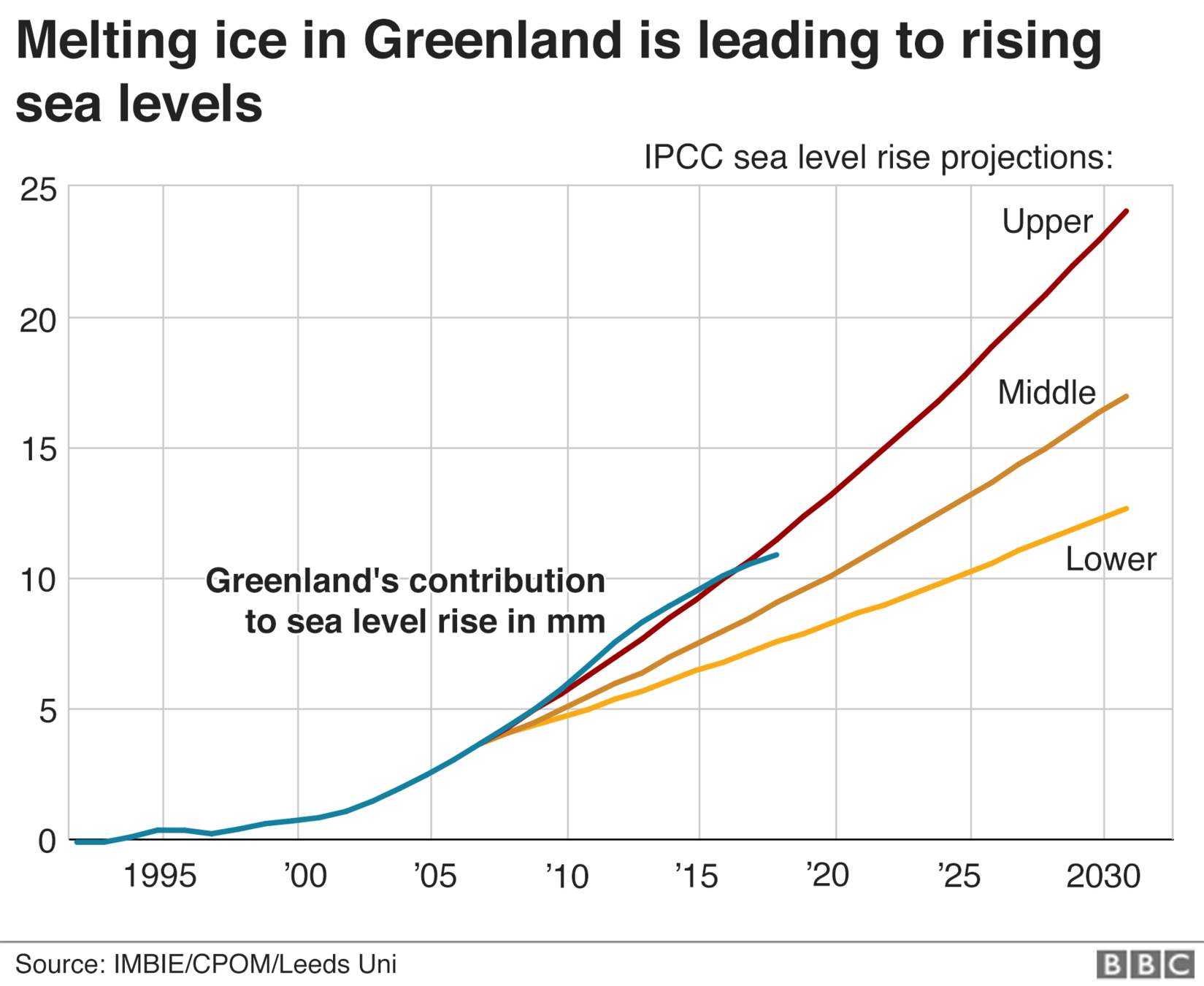
To predict and forecast
time (year)
See level contribution (mm)
Linear Regression
To explain
distance / age of the Universe
Universe's expansion rate
supernova (stellar explosion)
measure the expansion rate at the Universe as a function of time.
Deviation from linear falsify an adiabatically expanding Universe
time (year)
WHY?
Fitting a line
ax+b
to data y
To predict and forecast
See level contribution (mm)
Linear Regression
Key Concept
Model Fitting
We fit models to data in order to:
Predict and forecast: predict the value of the endogenous (dependent) variable at locations of the exogenous (independent, time) variable where we have no observations. This can be within the observed range, or outside of the range, which in time-series means predict the future (forecast)
Explain: relate observed behavior to first principles or behavior of possibly variables to explain the evolution and assess causality.
E.g. fitting a parabola to a bouncing ball demonstrates that gravity (and initial velocity) explains the behavior
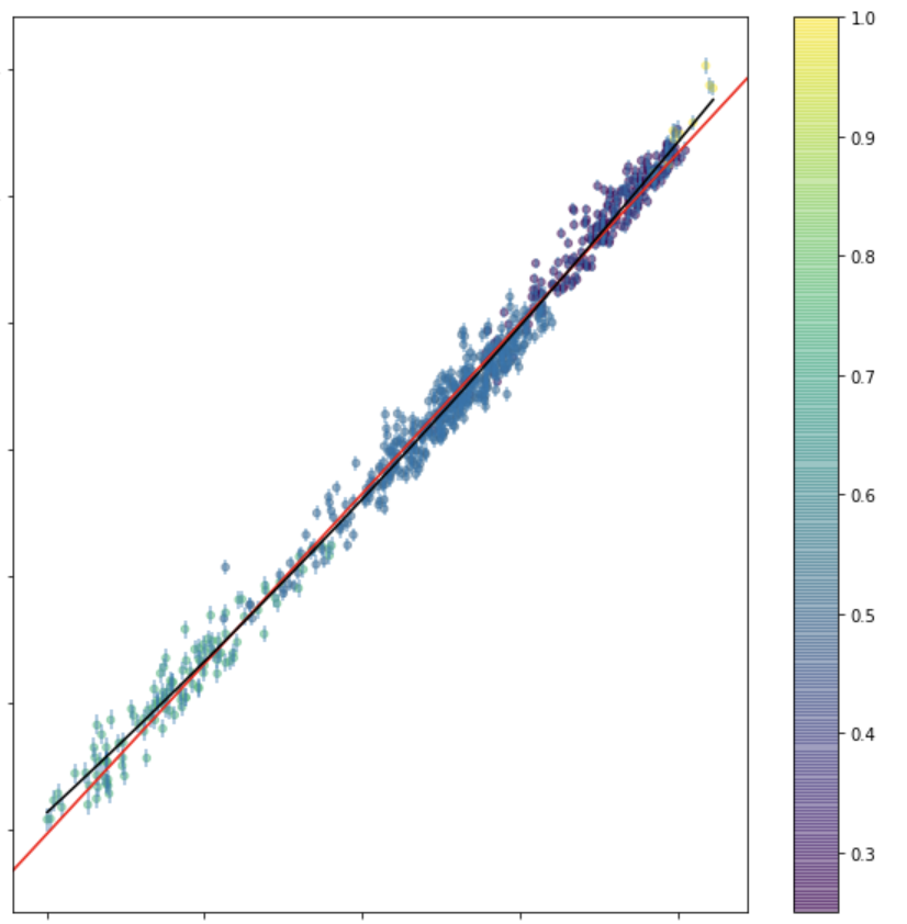
analytical solution
3.0
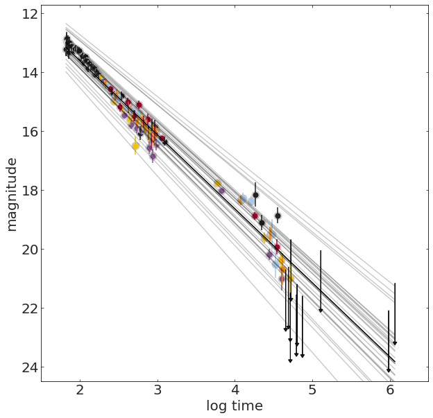
It can be shown that the optimal parameters for a line fit to data without uncertainties is:
X = np.c_[np.ones((len(grbAG) - grbAG.upperlimit.sum(), 1)),
	grbAG[grbAG.upperlimit == 0].logtime]
y = grbAG.loc[grbAG.upperlimit == 0].mag

theta_best = np.linalg.inv(X.T.dot(X)).dot(X.T).dot(y)It can be shown that the optimal parameters for a line fit to data without uncertainties is:
2xN Nx2 2xN Nx1
X = np.c_[np.ones((len(grbAG) - grbAG.upperlimit.sum(), 1)),
	grbAG[grbAG.upperlimit == 0].logtime]
y = grbAG.loc[grbAG.upperlimit == 0].mag

theta_best = np.linalg.inv(X.T.dot(X)).dot(X.T).dot(y)
It can be shown that the optimal parameters for a line fit to data without uncertainties is:
from sklearn.linear_model import LinearRegression
lr = LinearRegression()

X = np.c_[np.ones((len(grbAG) -
	grbAG.upperlimit.sum(), 1)),
	grbAG[grbAG.upperlimit == 0].logtime]
y = grbAG.loc[grbAG.upperlimit == 0].mag
lr.fit(X, y)
lr.coef_, lr.intercept_
We can let sklearn solve the equation for us:
2x1
2xN Nx2 2xN Nx1
X = np.c_[np.ones((len(grbAG) - grbAG.upperlimit.sum(), 1)),
	grbAG[grbAG.upperlimit == 0].logtime]
y = grbAG.loc[grbAG.upperlimit == 0].mag

theta_best = np.linalg.inv(X.T.dot(X)).dot(X.T).dot(y)Linear Correlation
3.1
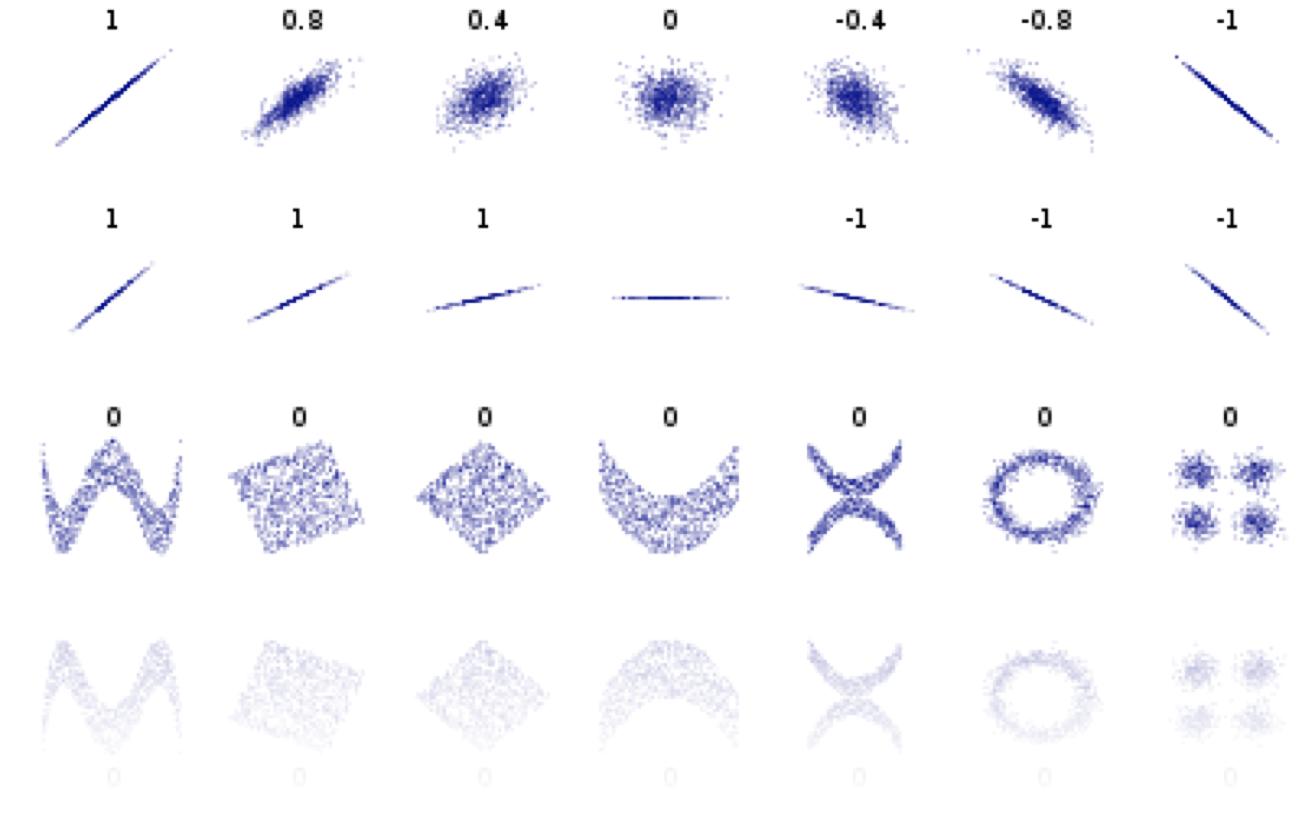
Pearson's correlation
Pearson's correlation measures linear correlation
Pearson's correlation
Pearson's correlation measures linear correlation
correlated
"positively" correlated
Pearson's correlation
Pearson's correlation measures linear correlation
correlated
"positively" correlated
Pearson's correlation
Pearson's correlation measures linear correlation
anticorrelated
"negatively" correlated
Pearson's correlation
Pearson's correlation measures linear correlation
anticorrelated
"negatively" correlated
Pearson's correlation
Pearson's correlation measures linear correlation
not linearly correlated
Pearson's coefficient = 0
does not mean that x and y are independent!
Pearson's correlation
Spearman's test
(Pearson's for ranked values)
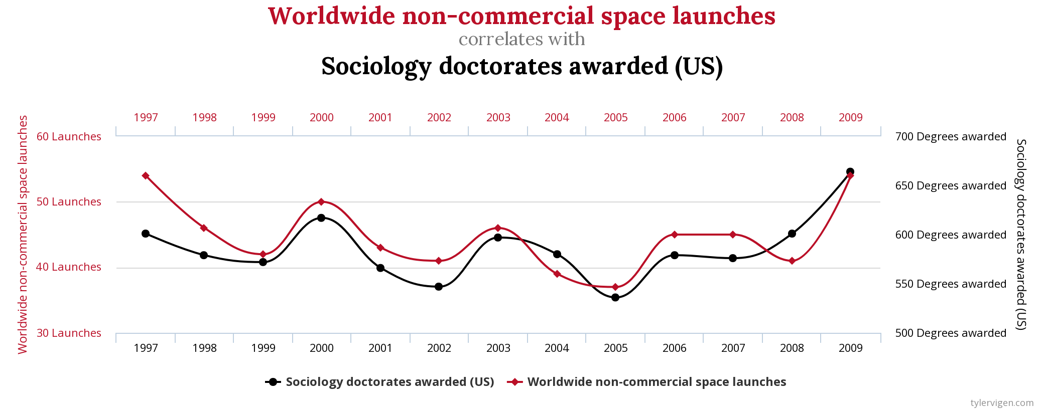
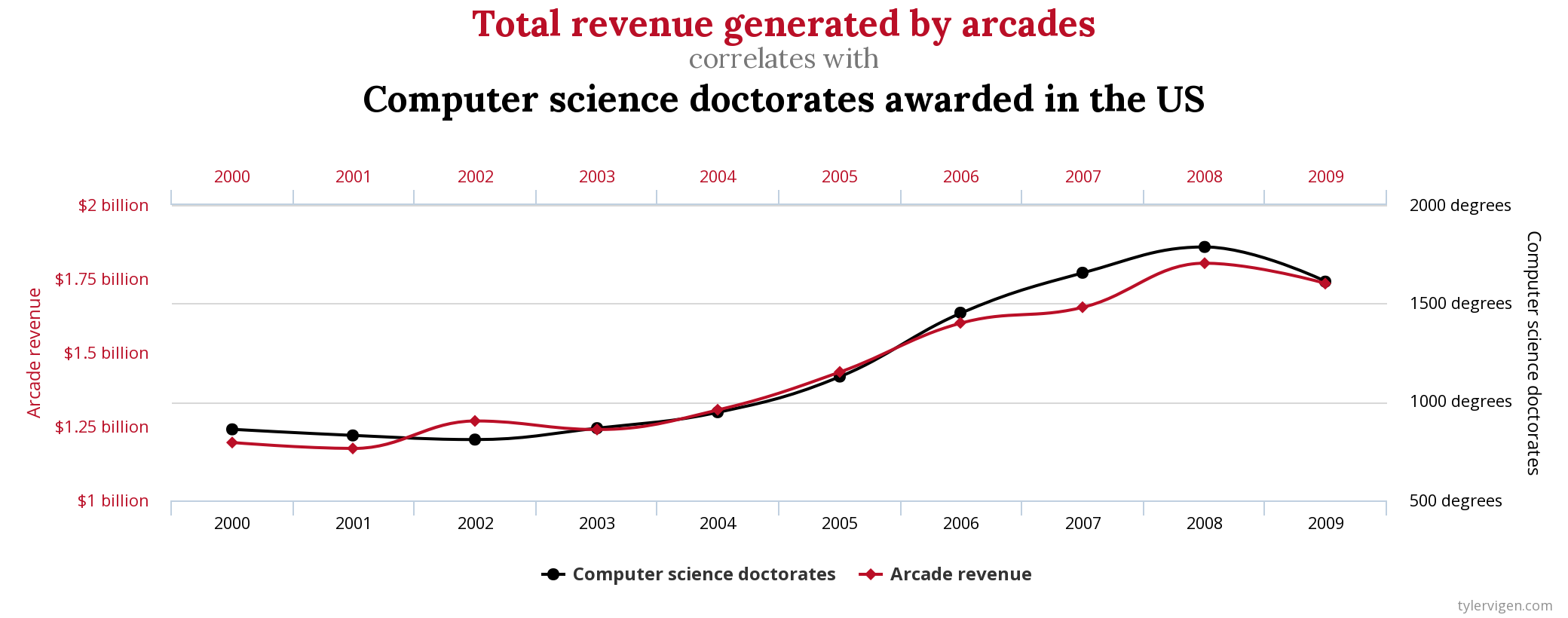
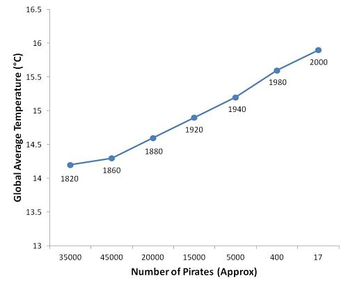
Correlation does not imply causality!!
2 things may be related because they share a cause but not cause each other:
icecream sales with temperature |death by drowning
with temperature
In the era of big data you may encounter truly spurious correlations
divorce rate in Maine | consumption of Margarine
Pearson's correlation
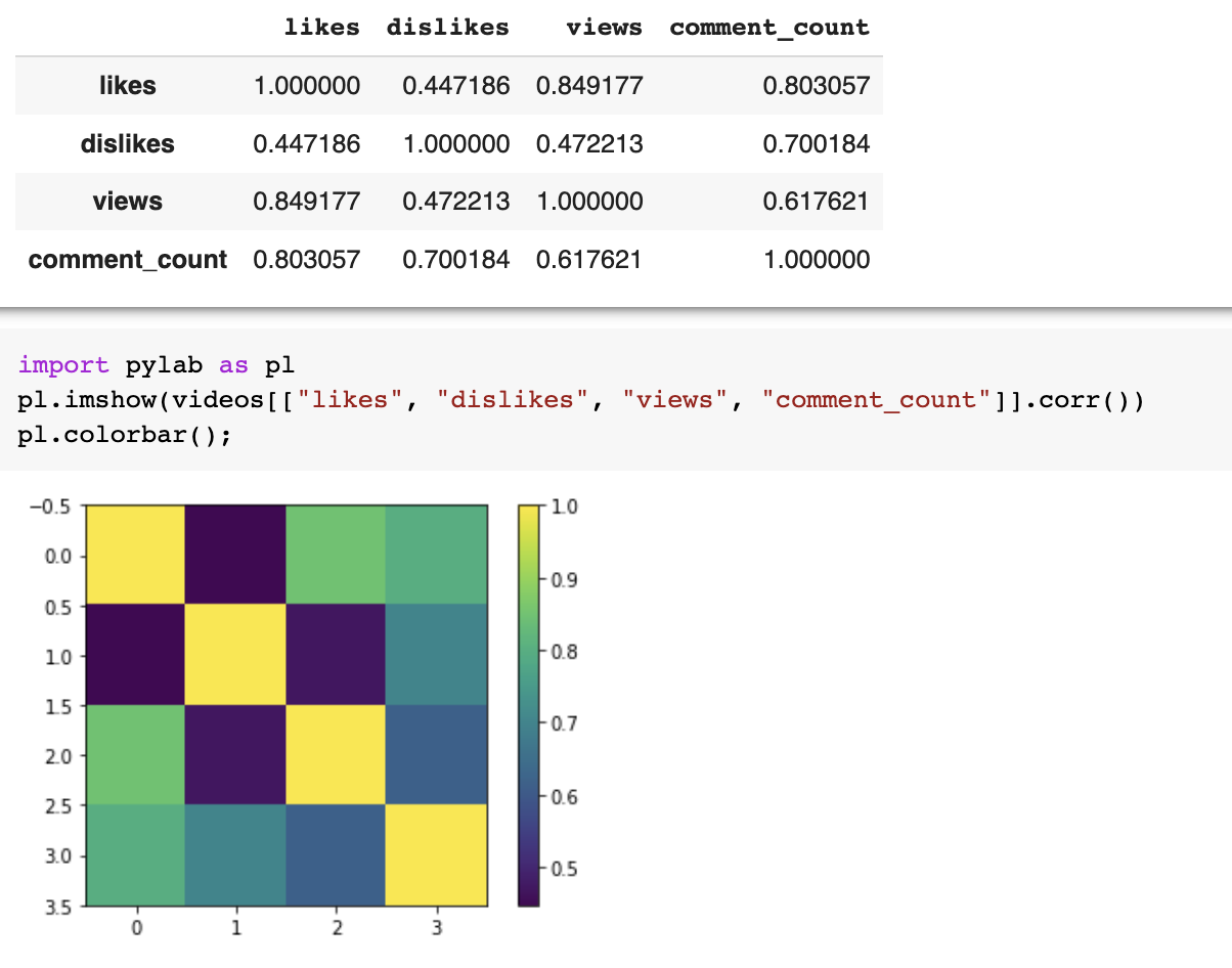
import pandas as pd
df = pd.read_csv(file_name)
df.corr()import pandas as pd
df = pd.read_csv(file_name)
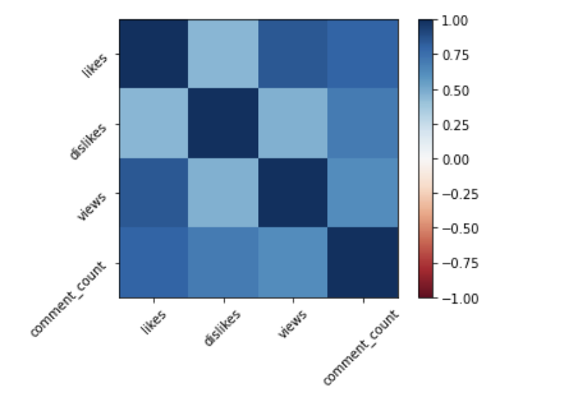
df.corr()pl.imshow(vdf.corr(), clim=(-1,1), cmap='RdBu')
pl.xticks(list(range(len(df.corr()))),
df.columns, rotation=45)
pl.yticks(list(range(len(df.corr()))),
df.columns, rotation=45)
pl.colorbar();<- anticorrelated | correlated ->
Pearson's correlation
import pandas as pd
df = pd.read_csv(file_name)
df.corr()import pandas as pd
df = pd.read_csv(file_name)
df.corr()pl.imshow(vdf.corr(), clim=(-1,1), cmap='RdBu')
pl.xticks(list(range(len(df.corr()))),
df.columns, rotation=45)
pl.yticks(list(range(len(df.corr()))),
df.columns, rotation=45)
pl.colorbar();objective function
3.2
time
time
time
time
time
time
which is the "best fit" line? A , B, C, D?
A
B
C
D
time
time
time
which is the "best fit" line? A , B, C, D?
A
B
C
D
time
time
time
which is the "best fit" line? A , B, C, D?
A
B
C
D
time
time
time
which is the "best fit" line? A , B, C, D?
A
B
C
D
time
time
time
which is the "best fit" line? A , B, C, D?
A
B
C
D
time
time
time
chi square: relates to the likelihood if the distribution is Gaussian
from scipy.optimize import minimize
def line(x, b, a):
    return a * x + b
def fitfunc(args, x, y):
    a, b = args
    return sum((y - line(a, b, x))**2)

x = grbAG.logtime.values
y = grbAG.mag.values
initialGuess = (10, 1)

fitfunc(initialGuess, x, y)
solution = minimize(fitfunc, initialGuess, args=(x, y))from scipy.optimize import minimize
def line(x, b, a):
return a * x + b
def chi2(args, x, y, s):
a, b = args
return sum((y - line(x, b, a))**2 / s)
x = grbAG.logtime.values
y = grbAG.mag.values
s = grbAG.magerr.values
initialGuess = (10, 1)
fitfunc(initialGuess, x, y)
solution = minimize(chi2, initialGuess, args=(x, y, s))
solutionOptimizing the Objective Function
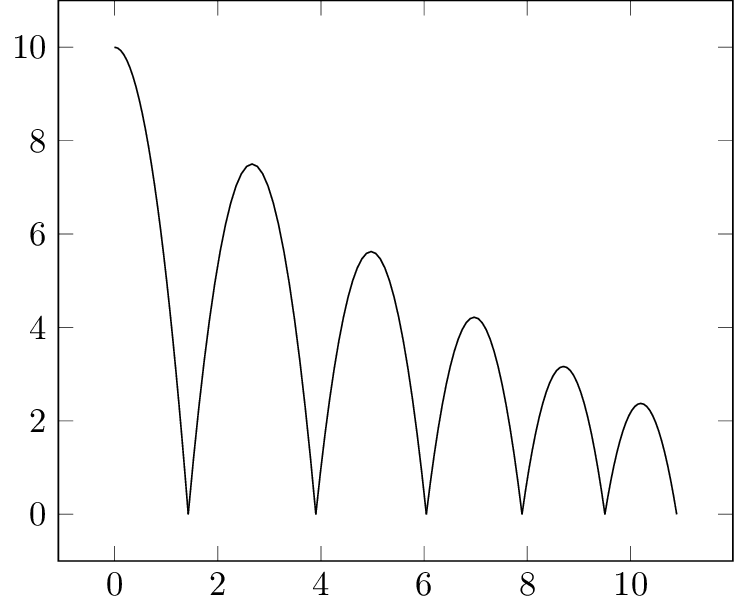
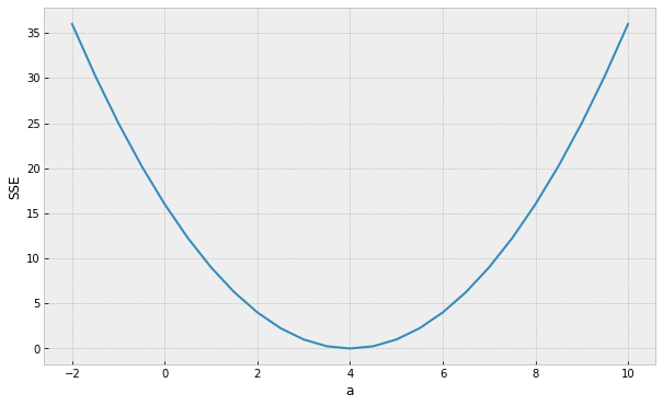
assume a simpler line model y = ax
(b = 0) so we only need to find the "best" parameter a
loss
assume a simpler line model y = ax
(b = 0) so we only need to find the "best" parameter a
Minimum (optimal) loss
a = 4
Optimizing the Objective Function
loss
assume a simpler line model y = ax
(b = 0) so we only need to find the "best" parameter a
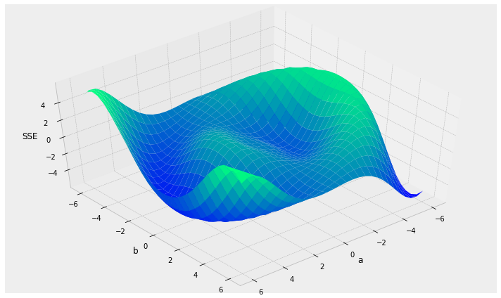
How do we find the minimum if we do not know beforehand how the SSE curve looks like?
Optimizing the Objective Function
Minimum (optimal) loss
a = 4
loss
3.1
stochastic gradient descent (SGD)
what is a machine learning?
1
2
3
4
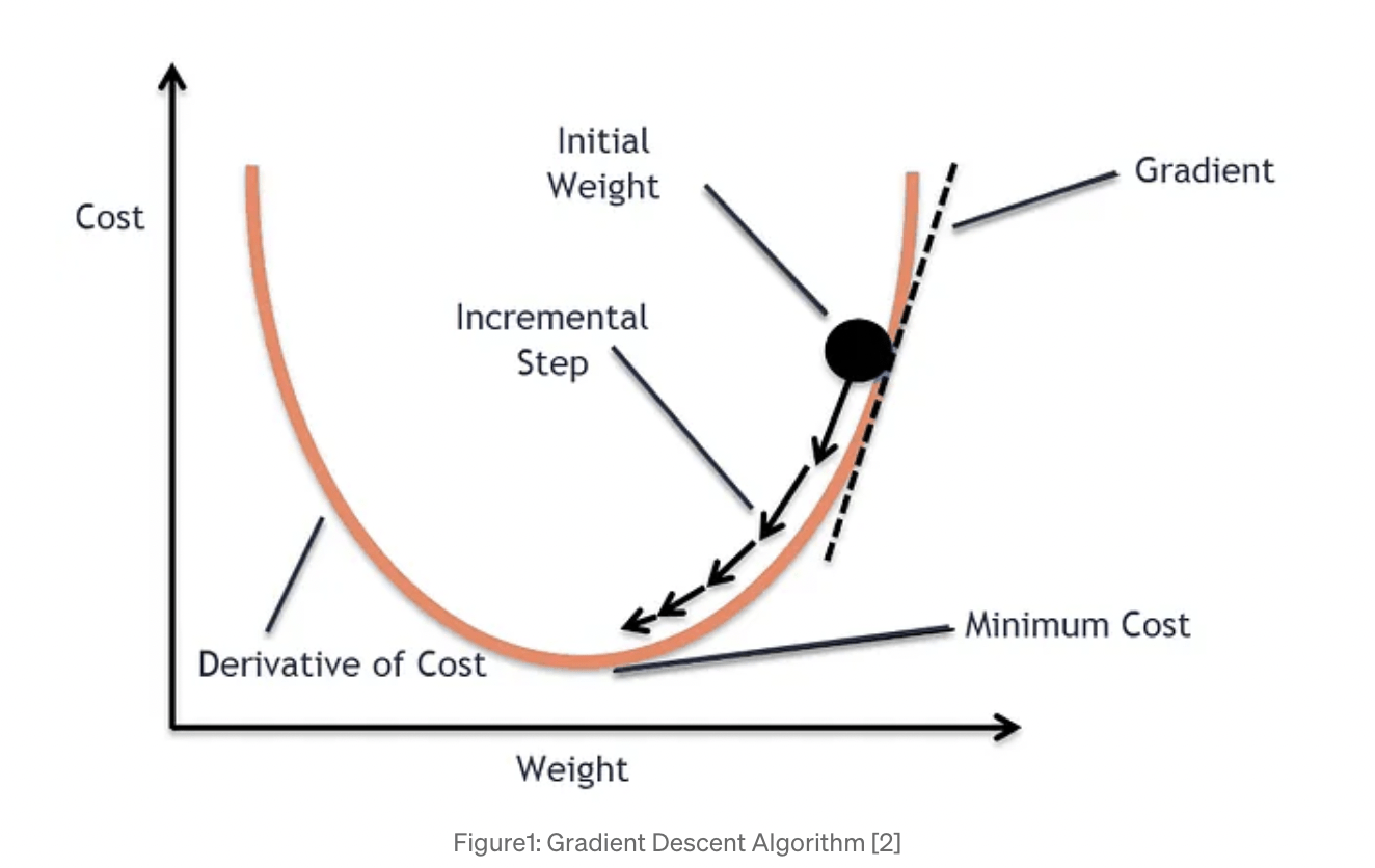
the algorithm: Stochastic Gradient Descent (SGD)
assume a simpler line model y = ax
(b = 0) so we only need to find the "best" parameter a
Minimum (optimal) loss
a = 4
loss
the algorithm: Stochastic Gradient Descent
assume a simpler line model y = ax
(b = 0) so we only need to find the "best" parameter a
1. choose initial value for a
-1
loss
the algorithm: Stochastic Gradient Descent
assume a simpler line model y = ax
(b = 0) so we only need to find the "best" parameter a
1. choose initial value for a=a0
2. calculate the loss at a0 : SSE(a0)
loss
the algorithm: Stochastic Gradient Descent
assume a simpler line model y = ax
(b = 0) so we only need to find the "best" parameter a
1. choose initial value for a=a0
2. calculate the loss at a0 : SSE(a0)
3. calculate best direction to go to decrease the SSE
loss
the algorithm: Stochastic Gradient Descent
assume a simpler line model y = ax
(b = 0) so we only need to find the "best" parameter a
1. choose initial value for a=a0
2. calculate the loss at a0 : SSE(a0)
3. calculate best direction to go to decrease the SSE
loss
the algorithm: Stochastic Gradient Descent
assume a simpler line model y = ax
(b = 0) so we only need to find the "best" parameter a
1. choose initial value for a=a0
2. calculate the loss at a0 : SSE(a0)
3. calculate best direction to go to decrease the SSE
loss
the algorithm: Stochastic Gradient Descent
assume a simpler line model y = ax
(b = 0) so we only need to find the "best" parameter a
1. choose initial value for a=a0
2. calculate the loss at a0 : SSE(a0)
3. calculate best direction to go to decrease the SSE
4. step in that direction
loss
the algorithm: Stochastic Gradient Descent
assume a simpler line model y = ax
(b = 0) so we only need to find the "best" parameter a
1. choose initial value for a=a0
2. calculate the loss at a0 : SSE(a0)
3. calculate best direction to go to decrease the SSE
4. step in that direction
5. go back to step 2 and repeat
loss
the algorithm: Stochastic Gradient Descent
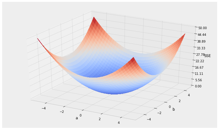
for a line model y = ax + b
we need to find the "best" parameters a and b
1. choose initial value for a & b
2. calculate the SSE(a0,b0)
3. calculate best direction to go to decrease the SSE
4. step in that direction
5. go back to step 2 and repeat
the algorithm: Stochastic Gradient Descent
for a line model y = ax + b
we need to find the "best" parameters a and b
1. choose initial value for a & b
2. calculate the SSE(a0,b0)
3. calculate best direction to go to decrease the SSE
4. step in that direction
5. go back to step 2 and repeat
the algorithm: Stochastic Gradient Descent
Things to consider:
loss
the algorithm: Stochastic Gradient Descent
Things to consider:
- local vs. global minima
local minima
global minimum
loss
the algorithm: Stochastic Gradient Descent
Things to consider:
- local vs. global minima
- initialization: choosing starting spot?
global minimum
local minima
loss
the algorithm: Stochastic Gradient Descent
Things to consider:
- local vs. global minima
- initialization: choosing starting spot?
- stopping criterion: when to stop?
loss
the algorithm: Stochastic Gradient Descent
Things to consider:
- local vs. global minima
Stochastic Gradient Descent (SGD): use a different (random) sub-sample of the data at each iteration
also: try different starting points and do multiple minimization (computationally expensive)
also: sometimes also go uphill (MonteCarlo methods)
loss
the algorithm: Stochastic Gradient Descent
Things to consider:
- local vs. global minima
- initialization: choosing starting spot?
- stopping criterion: when to stop?
- learning rate: how far to step?
loss
the algorithm: Stochastic Gradient Descent
Things to consider:
- local vs. global minima
- initialization: choosing starting spot?
- stopping criterion: when to stop?
- learning rate: how far to step?
the algorithm: Stochastic Gradient Descent
Things to consider:
- local vs. global minima
- initialization: choosing starting spot?
- stopping criterion: when to stop?
- learning rate: how far to step?
the algorithm: Stochastic Gradient Descent
Things to consider:
- local vs. global minima
- initialization: choosing starting spot?
- stopping criterion: when to stop?
- learning rate: how far to step?
the algorithm: Stochastic Gradient Descent
Things to consider:
- local vs. global minima
- initialization: choosing starting spot?
- stopping criterion: when to stop?
- learning rate: how far to step?
the algorithm: Stochastic Gradient Descent
assume a simpler line model y = ax
(b = 0) so we only need to find the "best" parameter a
1. choose initial value for a
2. calculate the SSE
3. take the gradient of the SSE and step in proportion
: the gradient is the slope of a line tangential to a point on a curve
the algorithm: Stochastic Gradient Descent
Things to consider:
- local vs. global minima
- initialization: choosing starting spot?
- stopping criterion: when to stop?
- learning rate: how far to step?
Adaptive learning rate: fast early on, slow later. Very common with Neural Networks
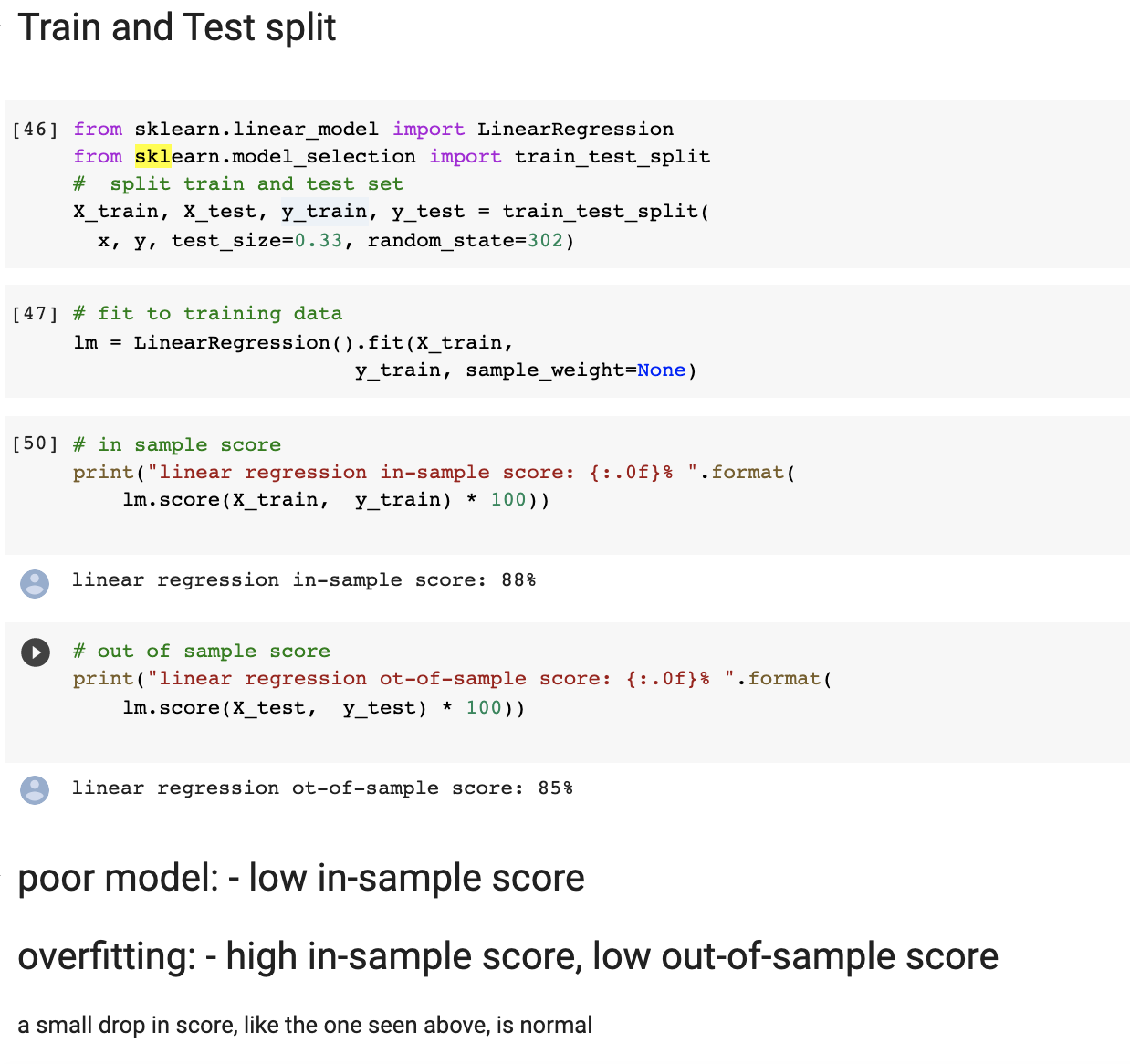
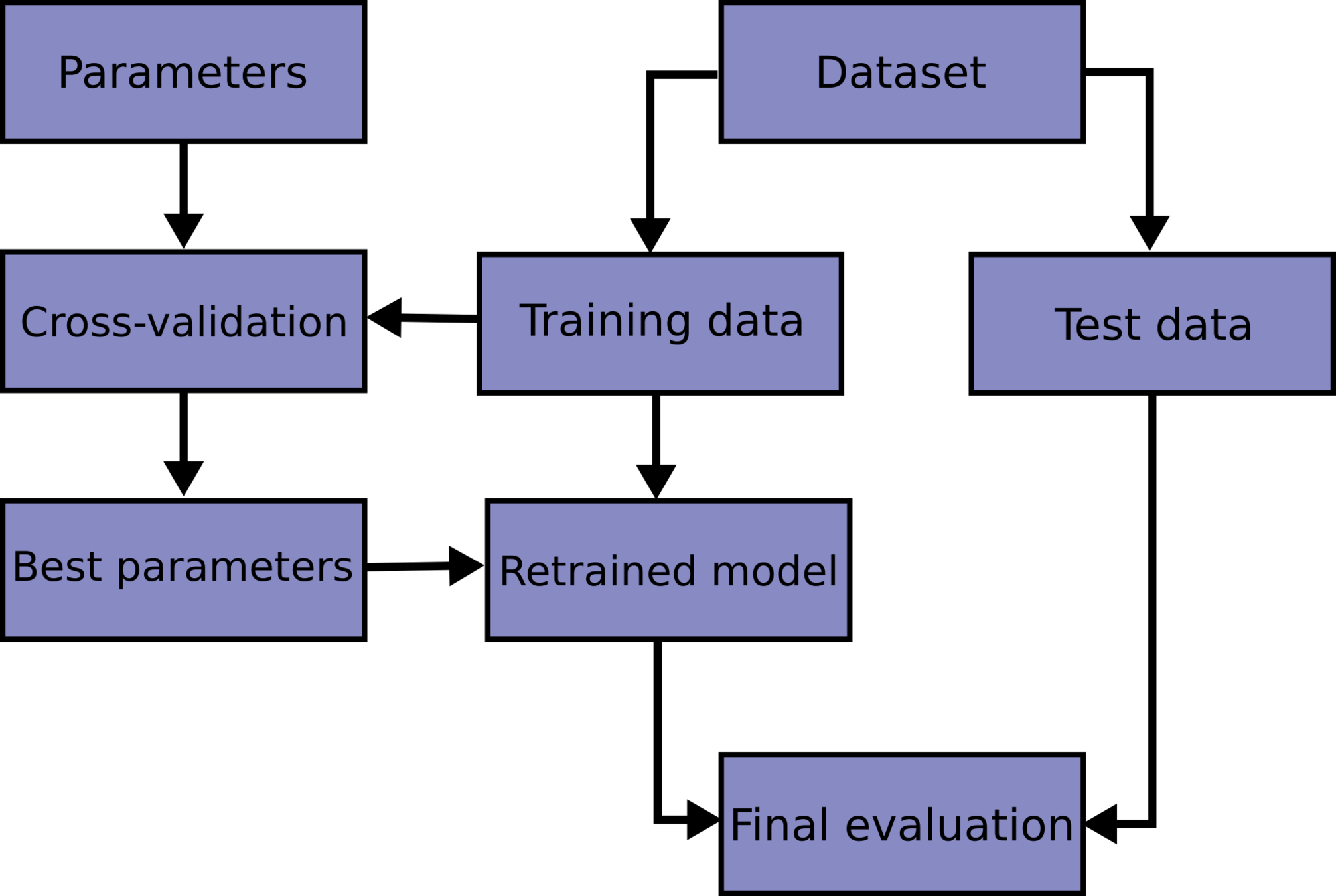
test train validation
train parameters on training set
run only once on the test set to assess the model performance
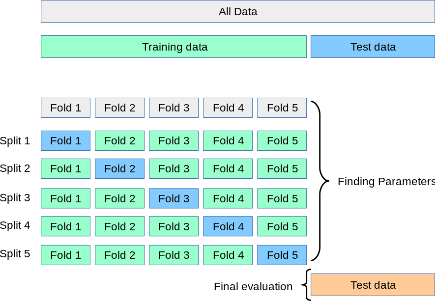
test + train + validation
train parameters on training set
adjust parameters on validation set
run only once on the test set to assess the model performance
k-fold cross validation
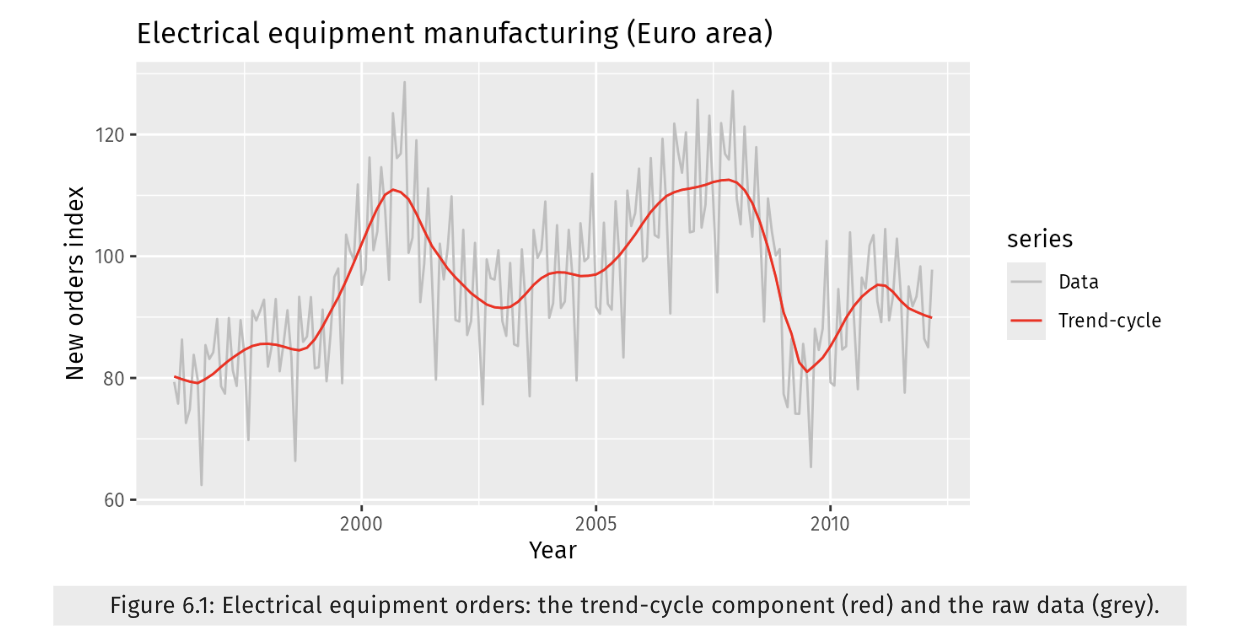
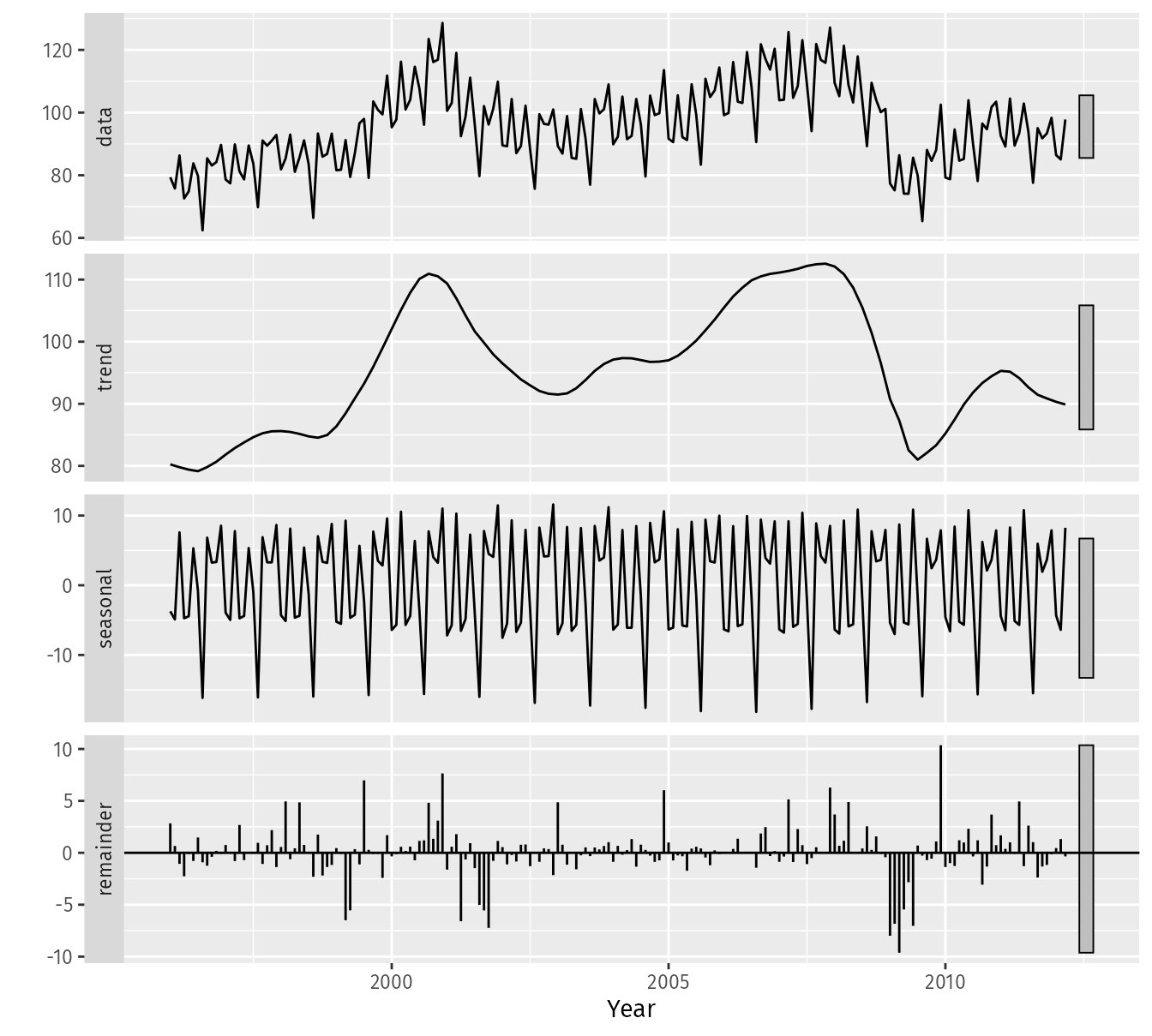
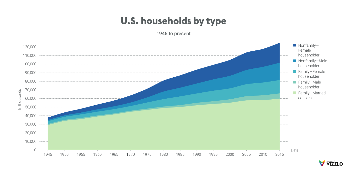
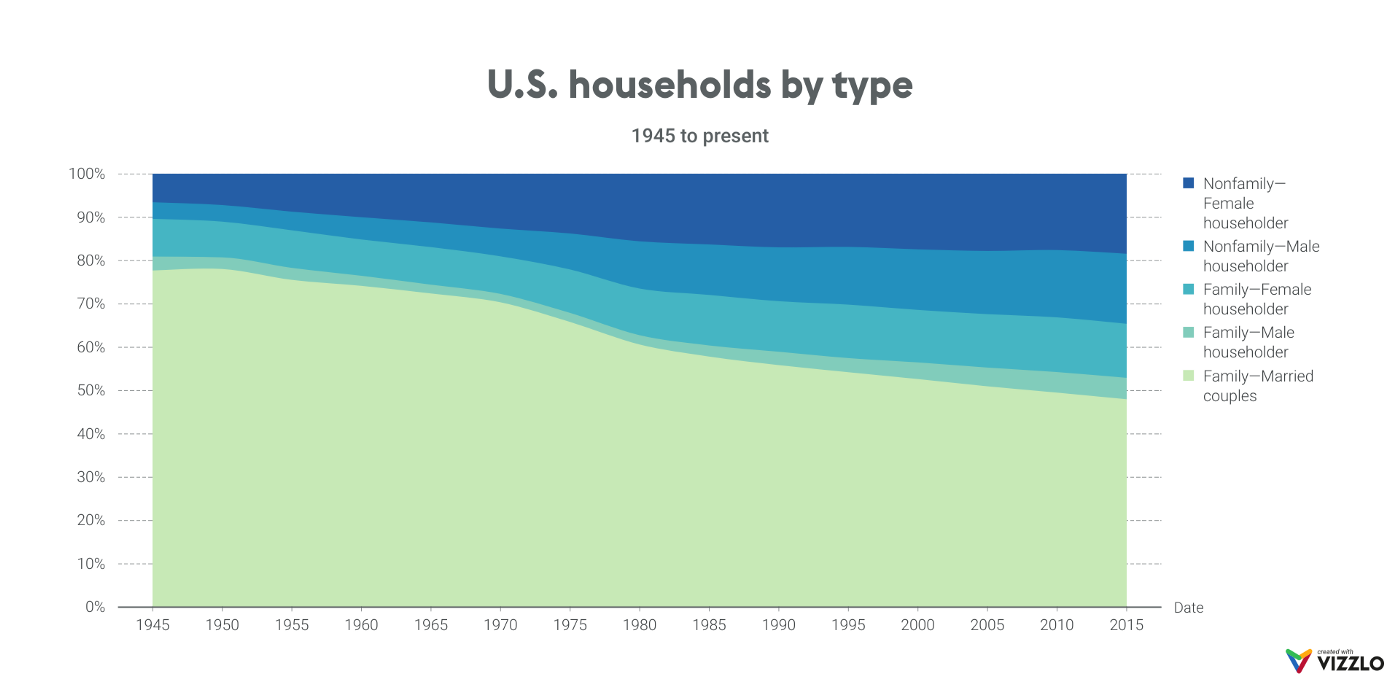
Time Series Components
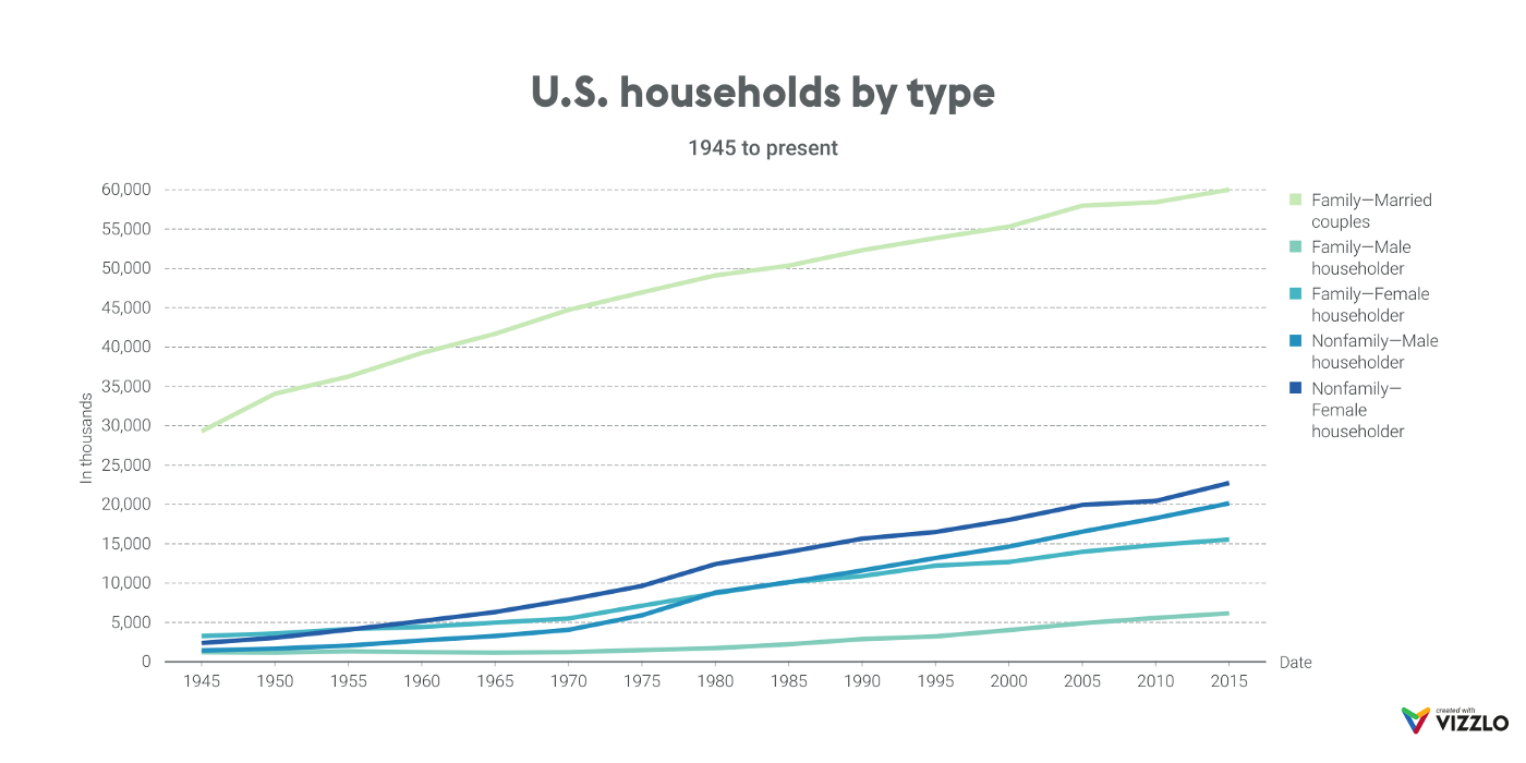
stacked area chart
Reproduciblity: A research product is reproducible if all numbers can be reproduced exactly be applying the same code to the same raw data. It is the responsibility of the researcher to provide the data and code that make a research product reproducible
What is Machine Learning? Machine Learning models are parametrized representations of "reality" where the parameters are learned from finite sets of realizations of that reality. Machine Learning is the discipline that conceptualizes, studies, and applies those models.
Model selection: Choosing a model i.e. a mathematical formula which we expect to be a simplified representation of our observations.
Objective Functions and optimization: To find the best model parameters we define a function of the data and parameters f(data, parameters) to be minimized or maximized.
Model fitting: Determining the best set of parameters to fit the observations within a chosen model.
Linear Regression as your ML first step: fitting a linear model (line or polynomial) to data is an approachable data analysis method that reveals _trends_ .
https://www.chi2innovations.com/blog/discover-stats-blog-series/graphs-prove-correlation-not-causation/
Correlation is not Causation
D. Hogg et al. https://arxiv.org/abs/1008.4686 - lots of details about how to properly treat outliers, uncertainties, assumptions in fitting a line to data. Witty comments make it entertaining. Exercise it make it very helpful
AstroML Chapter 10 - Intro
HOMLwSKLKerasTF Chapter 4 pages 111-117
Elements of Statistical Learning Chapter 3 Section 1 and 2
Intro and Chapter 1; pages 1-8
D. Hogg et al. https://arxiv.org/abs/1008.4686
Lots of details about how to properly treat outliers, uncertainties, assumptions in fitting a line to data. Witty comments make it entertaining. Exercise it make it very helpful
Falisifiability: A theory can be said to be scientific if it makes falsifiable predictions. Experiments should be designed to falsify the predictions
Reproduciblity: A research product is reproducible if all numbers can be reproduced exactly be applying the same code to the same raw data. It is the responsibility of the researcher to provide the data and code that make a research product reproducible
What is special about time series? Time series are series of exogenous-endogenous variable pairs where the exogenous variable is time, and therefore it is a sequential quantity with a specific direction of evolution.
What is Machine Learning? Machine Learning models are parametrized representations of "reality" where the parameters are learned from finite sets of realizations of that reality. Machine Learning is the discipline that conceptualizes, studies, and applies those models.
Objective Functions and optimization: To find the best model parameters we define a function of the data and parameters f(data, parameters) to be minimized or maximized.
Model fitting: Determining the best set of parameters to fit the observations within a chosen model.
D. Hogg et al. https://arxiv.org/abs/1008.4686 - lots of details about how to properly treat outliers, uncertainties, assumptions in fitting a line to data. Witty comments make it entertaining. Exercise it make it very helpful
AstroML Chapter 10 - Intro
HOMLwSKLKerasTF Chapter 4 pages 111-117
Elements of Statistical Learning Chapter 3 Section 1 and 2
By federica bianco
Linear Regression and Decomposition


