Fast computations of Wasserstein gradient flows
Joint works with Matt Jacobs and Wonjun Lee
Flavien Léger (inria)
Outline
1. Optimal transport
2. Wasserstein gradient flows
3. Numerical method
4. Movies
1. Optimal transport
2. Wasserstein gradient flows
3. Numerical method
4. Movies
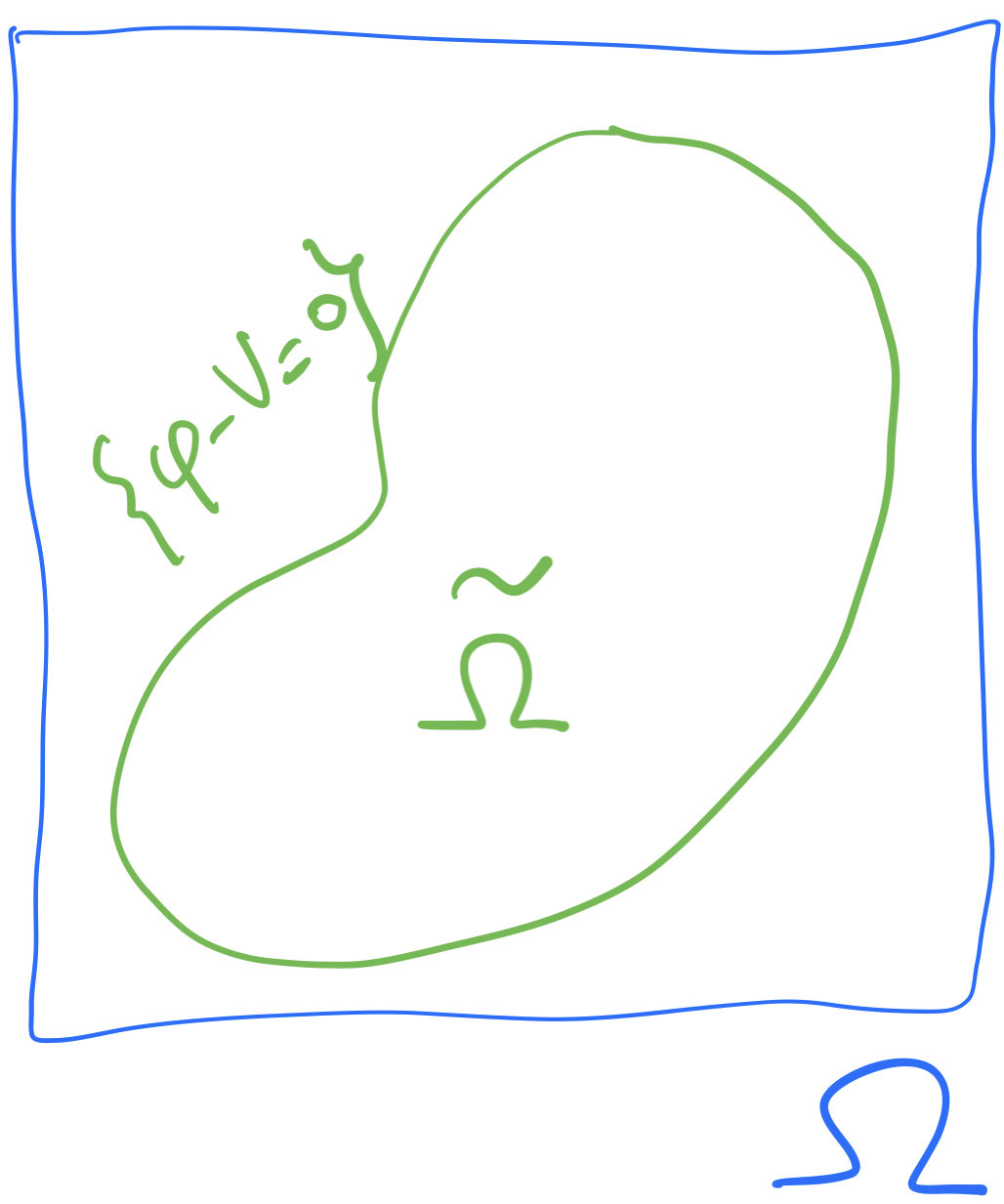
Setting
Two mass densities over \(\Omega\subset\mathbb{R}^d\), with same total mass,
\[\int_\Omega \mu(x)dx=\int_\Omega\nu(y)dy\]

\(\mu\)
\(\nu\)
How to optimally transport \(\mu\) to \(\nu\)?
Map \(T\colon\Omega\to\Omega\), measure \(\mu\)
Pushforward: \((T_{\#}\mu)(A)=\mu(T^{-1}(A))\)
D E F I N I T I O N
\(\mu\)
\(T_{\#}\mu\)
\(T(x)\)
$$\inf_{T}\int_\Omega |T(x)-x|^2 \,\mu(dx)=:W_2^2(\mu,\nu)$$
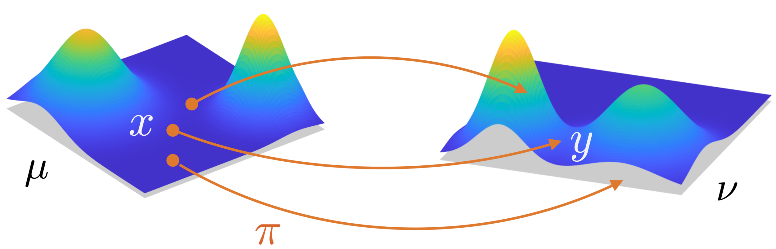
subject to: \(T_{\#}\mu=\nu\)
Cost to move mass \(\mu(dx)\) from \(x\) to \(T(x)\) is
\[|T(x)-x|^2 \,\mu(dx)\]
\(T(x)\)
$$\inf_{T}\int_\Omega |T(x)-x|^2 \,\mu(dx)=:W_2^2(\mu,\nu)$$
subject to: \(T_{\#}\mu=\nu\)
Features:
1) A distance between \(\mu\) and \(\nu\)
2) An optimal map \(T\)
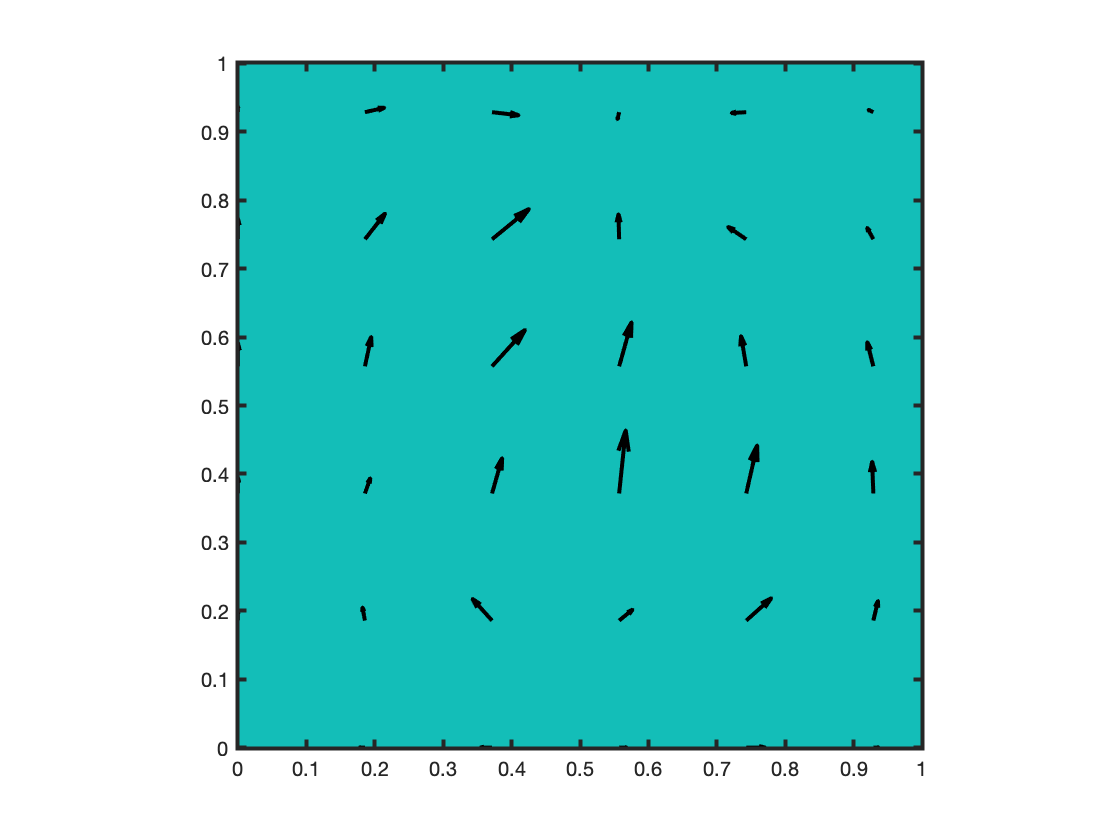
3) Formally a Riemannian metric on the manifold of measures with geodesics \[\rho_t = ((1-t)x+tT(x))_{\#}\mu\]
Numerically: not easy to solve
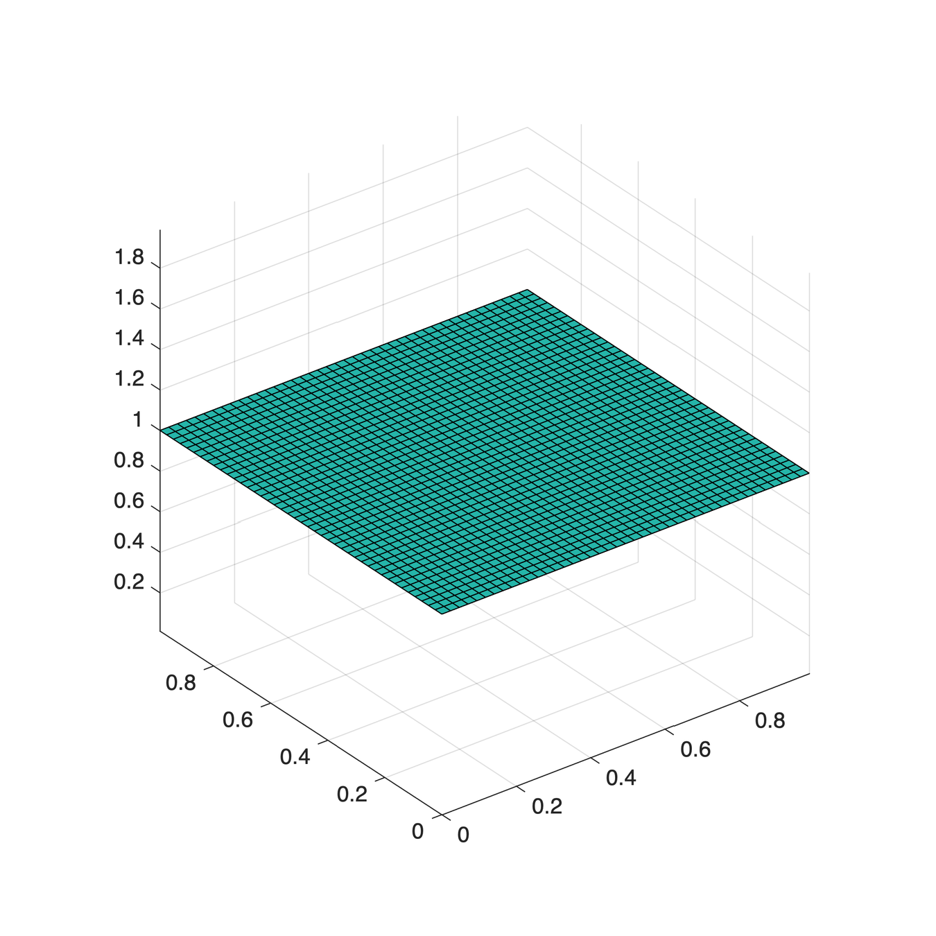
Example 1
\(2048\times 2048\) points
Example 2
Caffarelli's counterexample
\(2048\times 2048\) points
Summary
A distance \(W_2\) over measures, with “Riemannian” structure
1. Optimal transport
2. Wasserstein gradient flows
3. Numerical method
4. Movies
“\(\dot\rho_t = -\mathrm{grad}_{W_2}U(\rho_t)\)”
Functional \(U(\rho)\), want to make sense of
\[\rho(t+\tau)=\argmin_\rho U(\rho)+\frac{1}{2\tau}W_2^2(\rho(t),\rho)\]
Look at ”implicit Euler”
(JKO)
The right approach, theoretically and numerically
The PDEs
\[\partial_t\rho+\mathrm{div}(\rho\, v)=0,\]
\[v =-\nabla\phi,\]
\[\phi=\delta U(\rho)\]
on domain \(\Omega\subset\mathbb{R}^d\), no flux out and with initial condition \(\rho(t=0)=\rho_0\).
When \(\tau\to 0\),
Slow diffusion
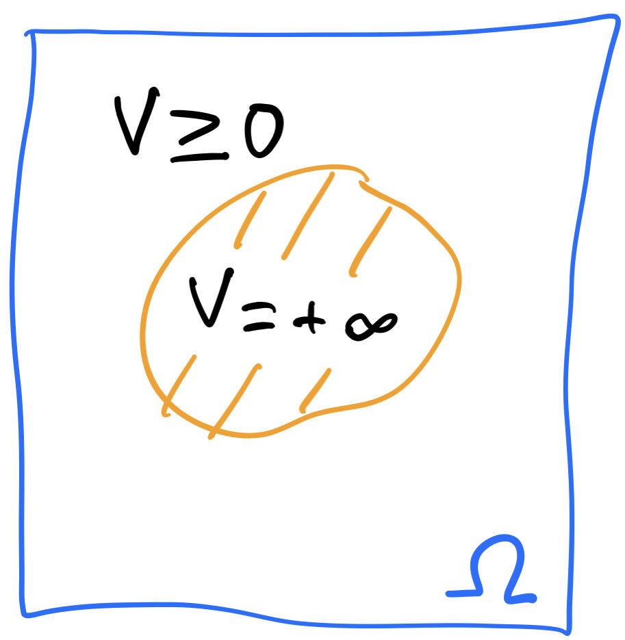
\[U(\rho)=\int_\Omega \frac{1}{m-1}\rho(x)^m+V(x)\rho(x)\,dx,\]
\(m > 1\). \(V(x)\) can be \(+\infty\).
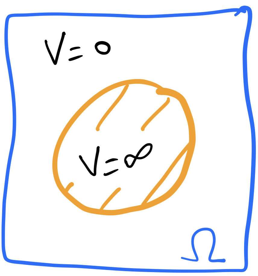
Incompressible energy
\[U(\rho)=\int_\Omega u_\infty(\rho(x))+V(x)\rho(x)\,dx,\]
Aggregation-diffusion
\[U(\rho)=\int_\Omega \rho(x)^m\,dx + \iint_\Omega |x-y|^2\rho(x)\rho(y)\,dxdy\]
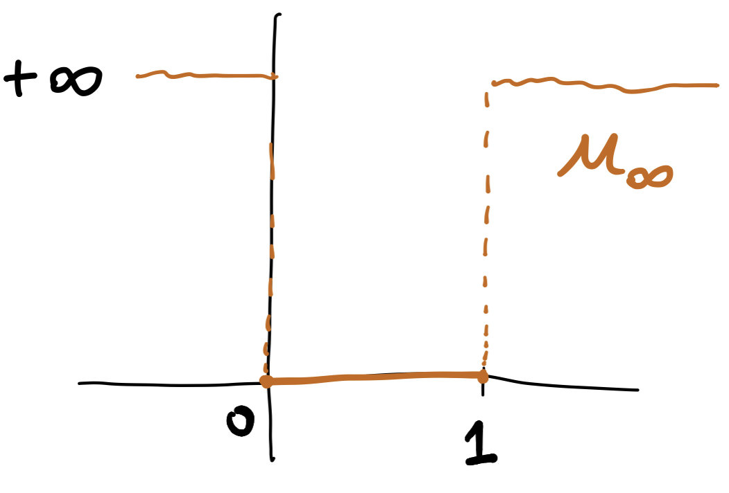
u_\infty(\rho)=\begin{cases}
0\quad\text{if } 0\le \rho\le 1\\
+\infty\quad\text{otherwise}
\end{cases}
porous medium equation
\(\partial_t\rho=\Delta\rho^m\).
\(m\to 1: U(\rho) = \int_\Omega \rho\log\rho + V\rho\)
Dual formulation
Primal, numerically difficult:
\[\sup_{\phi,\psi}\,\langle\psi,\mu\rangle - U^*(\phi)\]
over \((\phi,\psi)\) s.t.
\[\psi(x)-\phi(y)\le\frac{|x-y|^2}{2\tau}.\]
\[\inf_\rho U(\rho)+\frac{1}{2\tau}W_2^2(\mu,\rho).\]
Dual:
Dual formulations
\displaystyle\sup_{\psi(x)-\phi(y)\le\frac{|x-y|^2}{2\tau}}\langle\psi,\mu\rangle - U^*(\phi)
with \(\phi^c(x)=\inf_y\phi(y)+\frac{|x-y|^2}{2\tau}\),
\(\psi^c(y)=\sup_x\psi(x)-\frac{|x-y|^2}{2\tau}\).
☇
\[\sup_\phi\langle\phi^c,\mu\rangle-U^*(\phi)=:J(\phi)\]
\[\sup_\psi\langle\psi,\mu\rangle-U^*(\psi^c)=:I(\psi)\]
Dual formulations
→ unconstrained concave maximization problems
→ Recover \(\rho^*\) from \(\phi^*\) by
\[\rho^*=\delta U^*(\phi^*)\]
\[\sup_\phi\langle\phi^c,\mu\rangle-U^*(\phi)=:J(\phi)\]
\[\sup_\psi\langle\psi,\mu\rangle-U^*(\psi^c)=:I(\psi)\]
The power of duality
\[U(\rho)=\int_\Omega u_\infty(\rho(x))+V(x)\rho(x)\,dx.\]
\(\rho(x)=(u^*_\infty)'(\phi(x)-V(x))\) guaranteed to be \(0\) on obstacle.
Remark
\[U^*(\phi)=\int_\Omega u^*_\infty(\phi(x)-V(x))\,dx\]
☇
Summary
- Wasserstein gradient flow: \[\inf_\rho U(\rho)+\frac{1}{2\tau}W_2^2(\mu,\rho)\]
- Dual problem is better behaved: \[\sup_\phi J(\phi)\] or \[\sup_\psi I(\psi)\]
1. Optimal transport
2. Wasserstein gradient flows
3. Numerical method
4. Movies
Back-and-forth algorithm
\(H\) is the Sobolev space
\[\|h\|_H^2=\int_\Omega \alpha_1|\nabla h(x)|^2+\alpha_2|h(x)|^2\,dx\]
\begin{aligned}
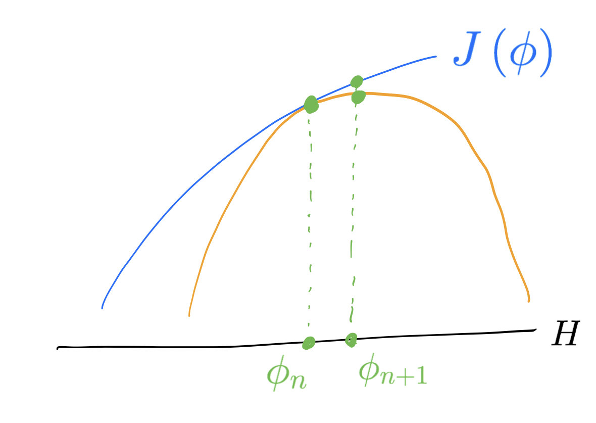
\phi_{k+\frac 1 2}&=\phi_k+\nabla_{\!H}J(\phi_k),\\
\psi_{k+\frac 1 2}&=(\phi_{k+\frac 1 2})^c,\\
\psi_{k+1}&=\psi_{k+\frac 1 2}+\nabla_{\!H}I(\psi_{k+\frac 1 2}),\\
\phi_{k+1} &= (\psi_{k+1})^c
\end{aligned}
\[J(\phi)=\langle\phi^c,\mu\rangle-U^*(\phi)\]
\[I(\psi)=\langle\psi,\mu\rangle-U^*(\psi^c)\]
Recall
Jacobs, Lee, L. (’21)
A L G O R I T H M
Why \(H\) ?
Assume that
$$0\le -\delta^2\!J(\phi)(h,h) \le \lVert h\rVert_H^2$$
for any \(\phi,h\in H\). Then the iterations
$$\phi_{k+1}=\phi_k+\nabla_{\!H} J(\phi_k)$$
converge to the supremum of \(J\).
Fundamental lemma in optimization:
Why \(H\) ?
Want Hessian bound
\[0\le -\delta^2\!J(\phi)(h,h)\le \|h\|_H^2\]
\(J=F-U^*\) with \(F(\phi)=\int_\Omega\phi^c\,d\mu\).
$$ -\delta^2\!F(\phi)(h,h)=\tau\int_\Omega |\nabla h(x)|^2_{g(\phi)}\,(T_{\phi\#}\mu)(dx) $$
Why \(H\) ?
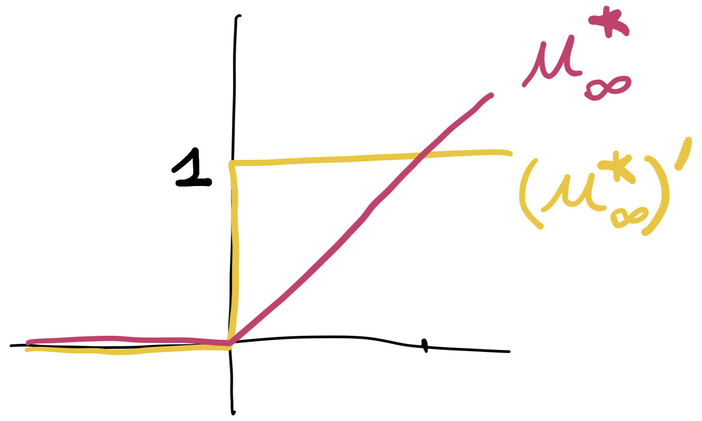
\[U^*(\phi)=\int_\Omega u^*_\infty(\phi(x))\,dx\]

\[\delta^2\!U^*(\phi)(h,h)\le C_\textrm{trace} \int_{\tilde\Omega} |\nabla h(x)|^2+|h(x)|^2\,dx\]
\[\delta^2U^*(\phi)(h,h)=\int_{\{\phi=0\}} |h(z)|^2\,d\sigma(z)\]
Back-and-forth is fast
\begin{aligned}
\phi_{k+\frac{1}{2}}&=\phi_k+(\Theta_1 - \Theta_2\Delta)^{-1}(T_{\phi_k\#}\mu - \delta U^*(\phi_k)) \\
\psi_{k+\frac{1}{2}}&=(\phi_{k+\frac{1}{2}})^c
\end{aligned}
Operations on a grid with \(N\) points:
- \(c\)-transform: \(O(N)\)
- \(T_{\phi_n} : O(N) \)
- \(\Delta^{-1}:O(N\ln N)\)
Summary
Novelty of the approach:
1) a careful analysis of the Hessian of the objective function
2) the back-and-forth scheme which boosts the convergence
4. Movies!
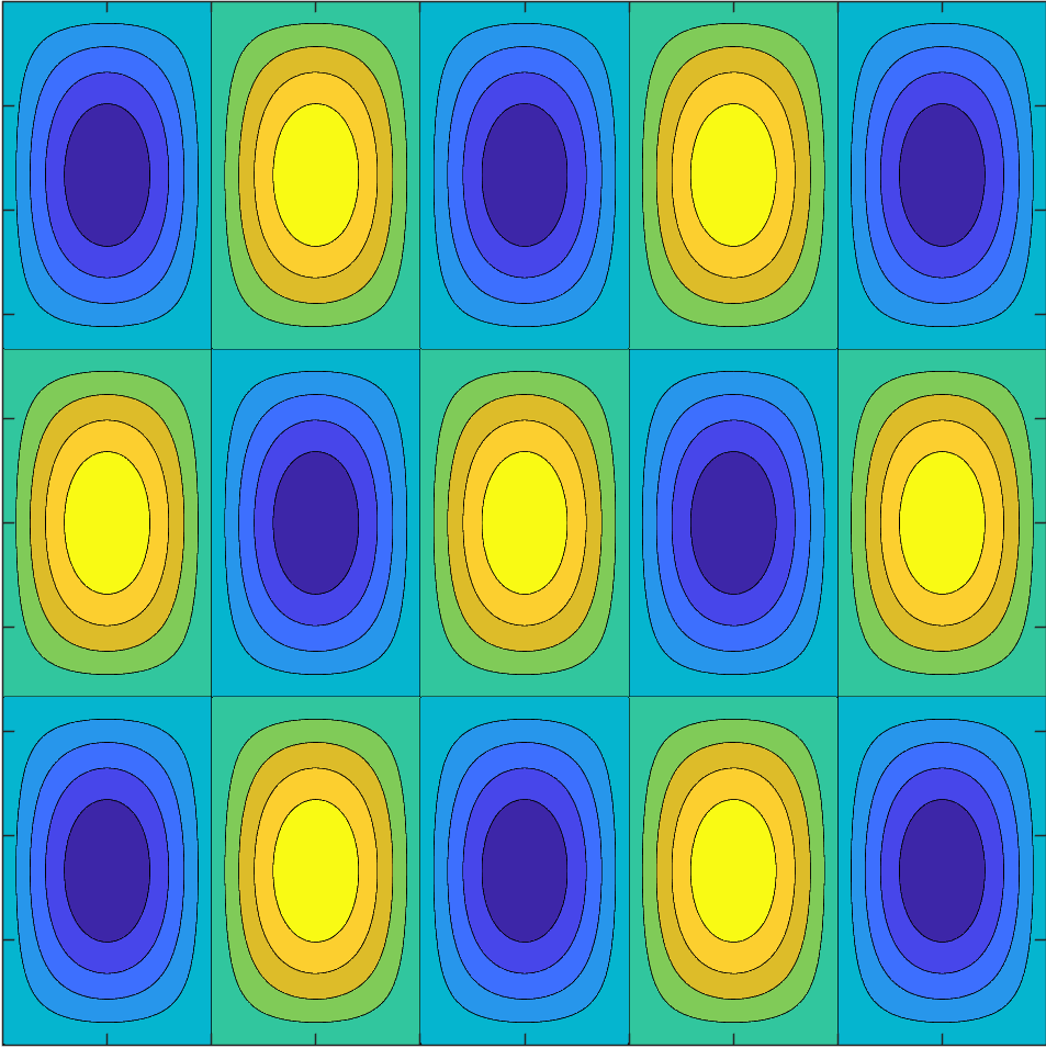
Slow diffusion (porous medium eq)
\(V(x)=-\sin(5\pi x_1)\sin(3\pi x_2)\)
\(512\times 512\) points
\(m=2\)
\(m=4\)
Slow diffusion
\(m=4\)
\(V(x)=\|x-a\|^2\)
\(512\times 512\) points
Incompressible
\(V(x)=\|x-a\|^2\)
\(1024\times 1024\) points
Aggregation-diffusion
\[U(\rho)=\int \rho(x)^3dx+\iint |x-y|^2\rho(x)\rho(y)\,dxdy\]
Thanks!
(inria-ljll 2021-12-06) Fast computations of Wasserstein gradient flows
By Flavien Léger


