Taylor expansions for entropic transport
Flavien Léger
joint work with:
Pierre Roussillon, François-Xavier Vialard and Gabriel Peyré
Background on optimal transport
$$\mathrm{OT}_0(\mu,\nu)=\inf_{\pi\in\Pi(\mu,\nu)}\iint c(x,y)d\pi(x,y)$$
Primal formulation
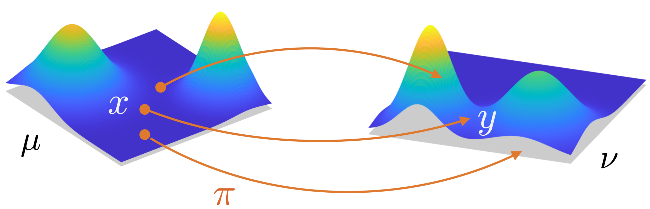
Optimal transport
\(\Pi(\mu,\nu)\): probability measures with marginals \(\mu\) and \(\nu\).
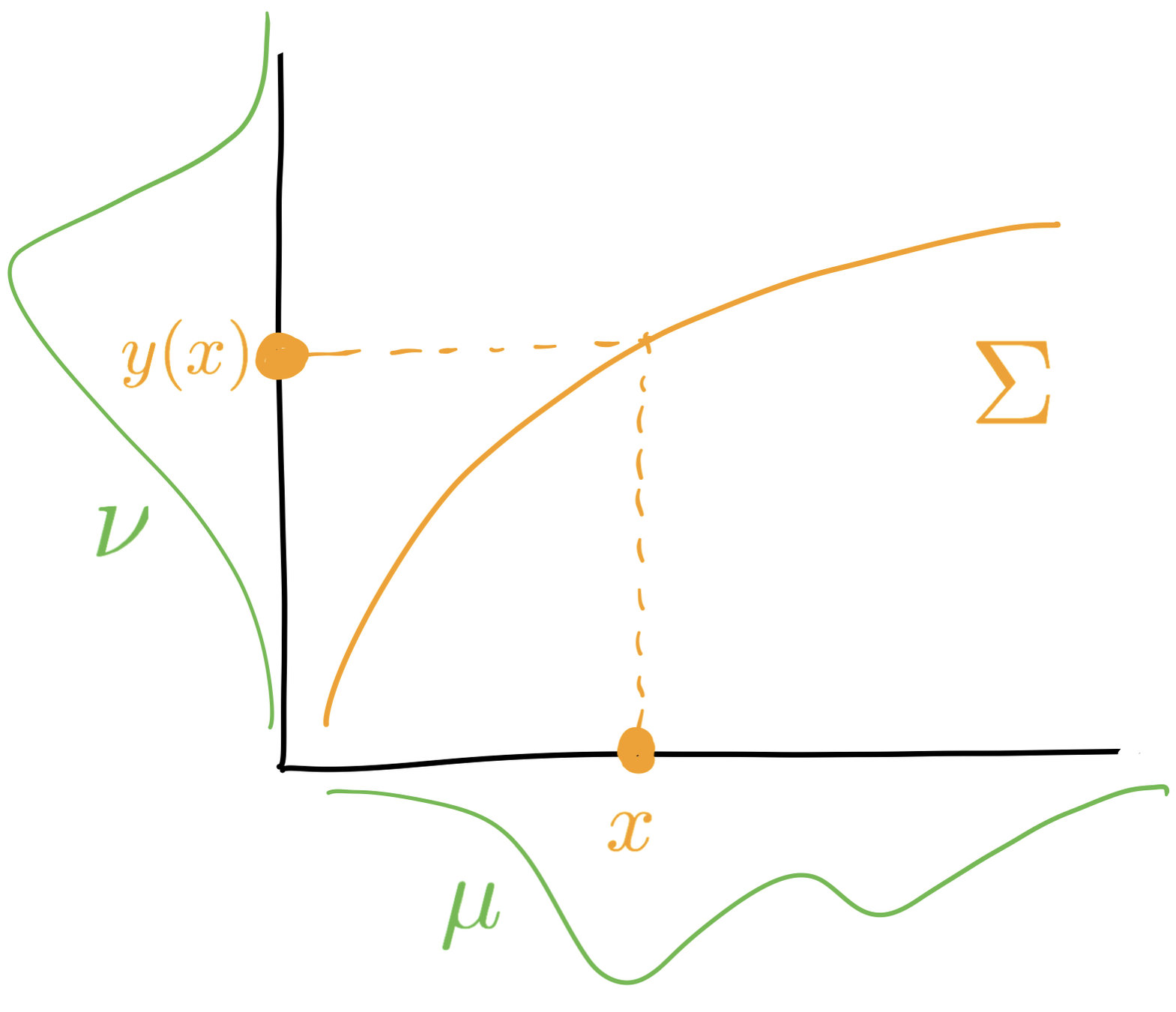
We assume that
$$\Sigma:=\mathrm{supp}\,\pi=\{(x,y(x)),x\in X\}$$
Optimal transport
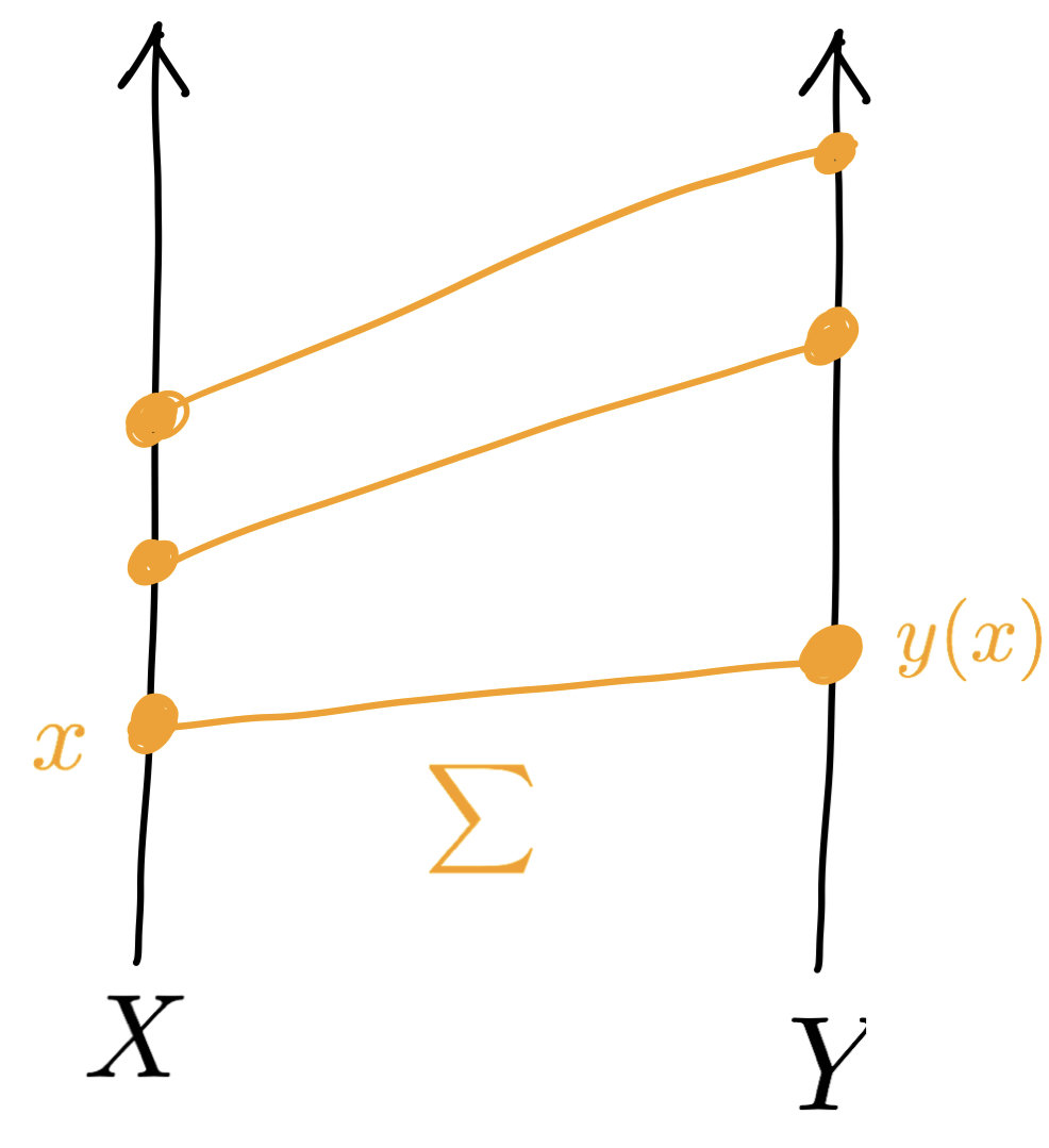
$$X$$
$$Y$$
Optimal transport
Dual formulation
$$\mathrm{OT}_0(\mu,\nu) = \sup_{\phi,\psi}\int\phi\,d\nu - \int\psi\,d\mu$$
s.t.
$$u(x,y):=c(x,y)+\psi(x)-\phi(y)\ge 0$$

The \(c\)-divergence
$$u(x,y)=c(x,y)+\psi(x)-\phi(y)\ge 0$$
$$\Sigma = \{(x,y) : u(x,y) = 0\}$$
Example: \(c(x,y)=-x\cdot y\)
$$u(x,y)=\psi(x)-\phi(y)-x\cdot y$$
$$=\psi(x|x(y))$$
Bregman divergence
$$\mathrm{OT}_\varepsilon(\mu,\nu)=\inf_{\pi\in\Pi(\mu,\nu)}\iint c(x,y)d\pi(x,y) + \varepsilon H(\pi|\mu\otimes\nu)$$
Entropic transport
Primal formulation
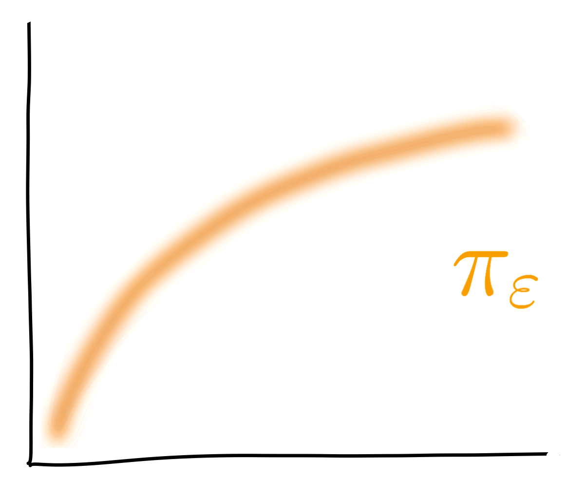
\(\pi_\varepsilon\) vs \(\pi_0\)?
Q U E S T I O N
$$X$$
$$Y$$
$$\mathrm{OT}_\varepsilon(\mu,\nu)=\sup_{\phi,\psi}\int\phi\,d\nu-\int\psi\,d\mu-\varepsilon\ln\Big(\iint e^{-\frac1\varepsilon (c+\psi-\phi)}d\mu d\nu\Big)$$
Dual formulation
Entropic transport
$$\longrightarrow \pi_\varepsilon(x,y) = e^{-\frac1\varepsilon(c(x,y)+\psi_\varepsilon(x)-\phi_\varepsilon(y))}\mu(x)\nu(y)$$
Solve with Sinkhorn: \(\phi^n \to \psi^n\to\phi^{n+1}\to\dots\)
Our question
\(\pi_0\) singular measure supported on \(\Sigma\)
\(\pi_\varepsilon\) smooth measure supported on \(X\times Y\)
$$\mathrm{OT}_0(\mu,\nu)$$
$$\mathrm{OT}_\varepsilon(\mu,\nu)$$


What's known
- In general $$\phi_\varepsilon\to\phi_0\quad\text{as }\varepsilon\to 0$$ (Nutz & Wiesel ’21, Berman ’21, N Gigli & L Tamanini ’18)
- For general costs $$\mathrm{OT}_\varepsilon(\mu,\nu)\approx\mathrm{OT}_0(\mu,\nu)-\varepsilon\ln(2\pi\varepsilon)^{d/2}-\varepsilon H(\nu|m)$$ (S Pal ’19)
- For quadratic costs (Schrödinger problems )$$\mathrm{OT}_\varepsilon(\mu,\nu)\approx\mathrm{OT}_0(\mu,\nu)-\varepsilon\ln(2\pi\varepsilon)^{d/2}-\frac\varepsilon 2(H(\mu)+H(\nu))$$ $$+\frac{\varepsilon^2}{8} \int_0^1 \mathrm{FI}(\rho_t)\,dt$$ (G Conforti & L Tamanini ’21)
Background on the Kim–McCann geometry
(YH Kim & RJ McCann ’10)
Riemannian metric \(g\) on \(\Sigma\)
$$c(x,y)+c(x+\xi,y+\eta) \le c(x+\xi,y)+c(x,y+\eta)$$
\(\lvert\xi\vert,\lvert\eta\rvert\ll 1\) yields
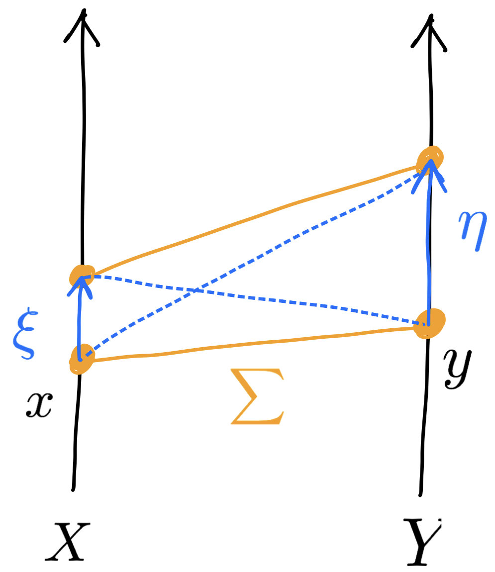
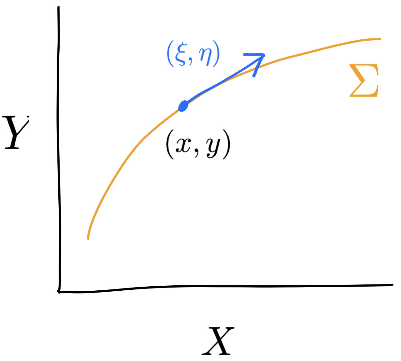
$$-D_{xy}^2c(x,y)(\xi,\eta)\ge 0$$
Quantifying a matching's stability
Kim and McCann's idea:
consider $$\hat g = -D^2_{xy}c$$ as a semi-metric over all \(X\times Y\)
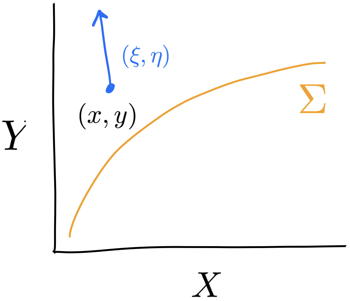
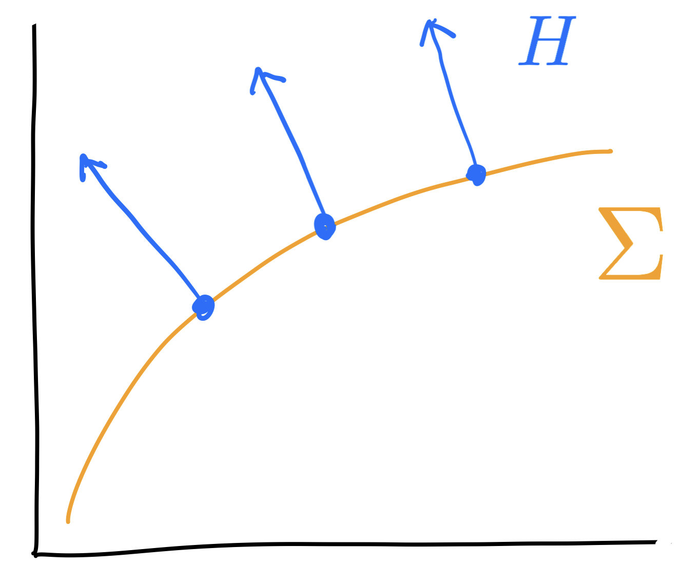
Second fundamental form
$$h(U,V)=(\hat\nabla_UV)^\perp$$
Mean curvature \(H=\mathrm{tr}(h)\) (a normal vector field)
$$(T\Sigma\times T\Sigma\to T^\perp\Sigma)$$
Additional structure: para-Kähler manifold
\((\cdot)^\perp\) maps \(T^\perp\Sigma\) to \(T\Sigma\)

Example: \(c(x,y)=-x\cdot y\)
$$\hat g=\begin{pmatrix}0&I_d\\I_d&0\end{pmatrix}$$
$$u(x,y)=\psi(x)-\phi(y)-x\cdot y$$
$$=\psi(x|x(y))$$
Bregman divergence
$$g=D^2\psi$$
Hessian metric
flat metric
In summary, we have
On \(X\times Y\)
On \(\Sigma\)
Extrinsic curvatures
\(\hat g\) semi-metric
\(\hat m\) volume form
\(\hat \nabla\) Levi-Civita connection
\(\hat R\) scalar curvature
\(g\) metric
\(m\) volume form
\(\nabla\) Levi-Civita connection
\(R\) scalar curvature
\(h\) second fundamental form
\(H\) mean curvature
A new Laplace formula
$$\iint_{X\times Y}\frac{e^{-u(x,y)/\varepsilon}}{(2\pi\varepsilon)^{d/2}}f(x,y)\,d\hat m(x,y) = \int_\Sigma fdm\,+$$
$$\varepsilon\int_\Sigma \bigg[-\frac 18\hat\Delta f+ \frac 14 \hat\nabla_{\!H} f+ \frac{1}{16}\Big( |H|^2 - \frac{5}{3}|h|^2 -R + \frac{3}{4}\hat R\Big)f\bigg] \,dm + \varepsilon^2\mathcal{R}(\varepsilon)$$
T H E O R E M
\(u\) vanishes on \(\Sigma\)
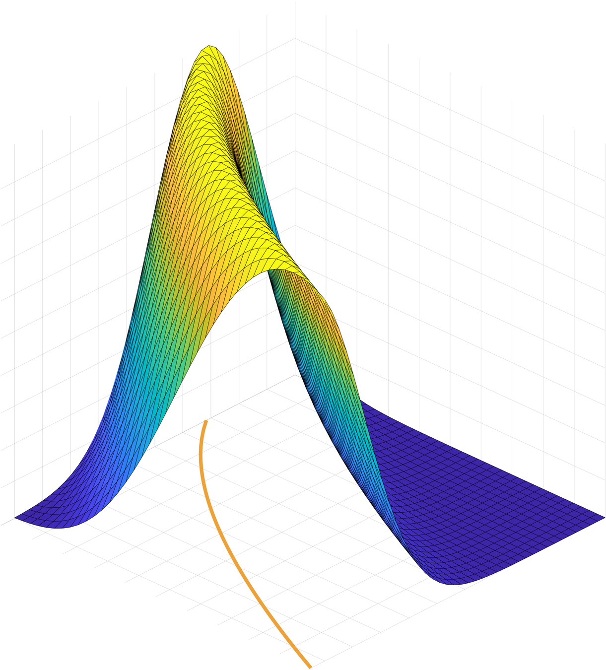
$$\Sigma$$
$$e^{-u(x,y)/\varepsilon}$$
$$X$$
$$Y$$
Assumptions:
$$X=Y=\mathbb{R}^d$$
$$0<\lambda\le D^2u\le\Lambda$$
$$f\textrm{ and } D^2u \in W^{4,\infty}$$
Novelties:
1. Geometric expression
2. Quantitative remainder bound
$$\lvert\mathcal{R}(\varepsilon) \rvert \le C \lVert D^2u\rVert_{W^{4,\infty}}^4 \iint_{X\times Y} \frac{e^{-\lambda\lvert y-y(x)\rvert^2/2\varepsilon}}{(2\pi\varepsilon/\lambda)^{d/2}} \lvert D_{\le 4}f\rvert (x,y)\,d\hat{m}(x,y)$$
Taylor expansion of the potentials
$$\mathrm{div}_\pi(\nabla V)=\mathrm{div}_\pi(H^\perp)$$
\(H\) : mean curvature, \(H^\perp\) tangent to \(\Sigma\)
Solve for \(V\) on \(\Sigma\)
\(\pi\) : optimal transport plan
(supported on \(\Sigma\))
$$\int_\Sigma \mathrm{div}_\pi(\xi) f\,d\pi = -\int_\Sigma\xi\cdot\nabla f\,d\pi$$
D E F I N I T I O N
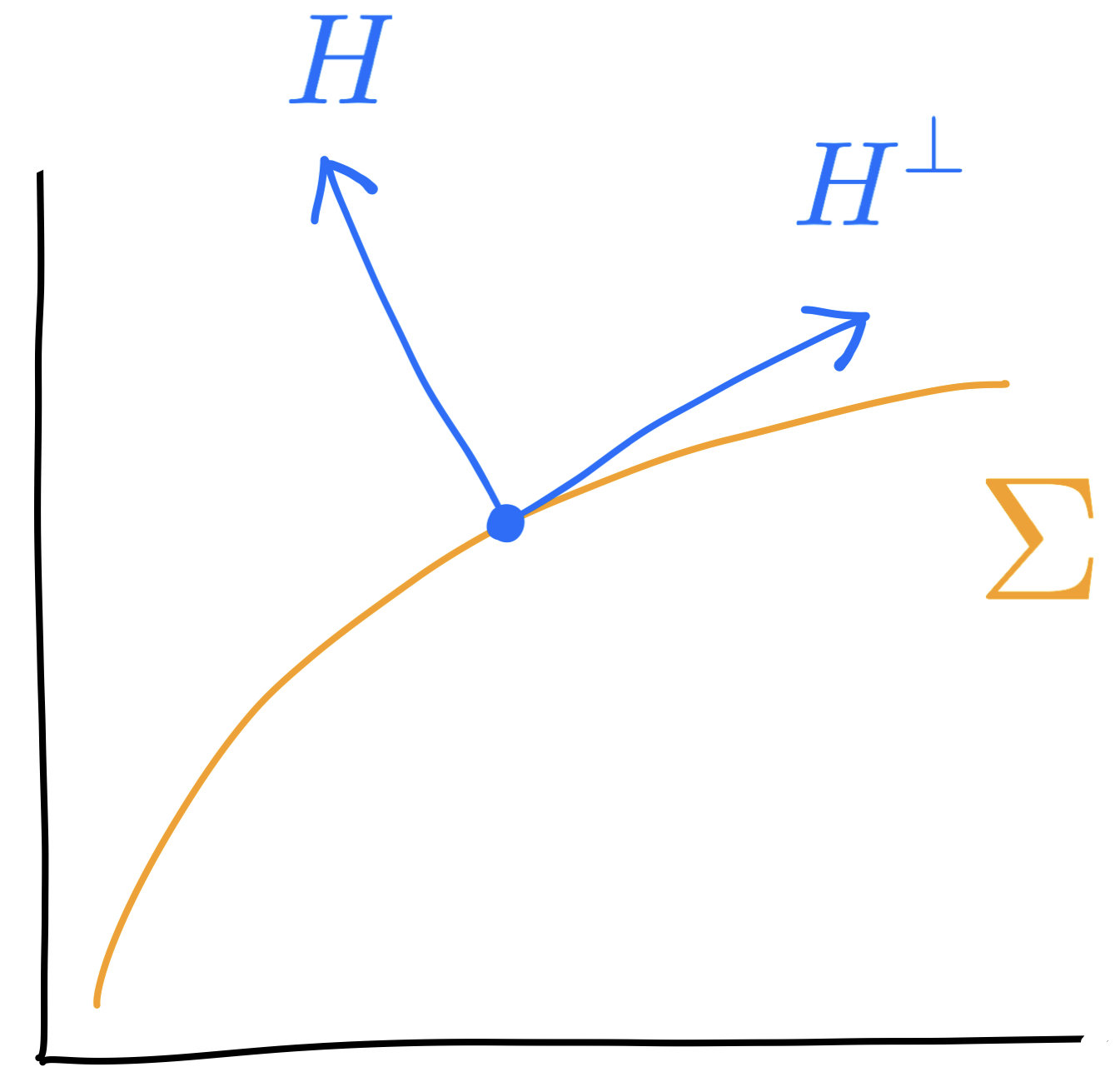
$$\mathrm{div}_\pi(\nabla V)=\mathrm{div}_\pi(H^\perp)$$
$$\psi_\varepsilon=\psi_0+\frac\varepsilon 2\ln\Big(\frac{m}{e^{-V}\mu}\Big) + o(\varepsilon)$$
T H E O R E M
$$u(x,y)\approx -\varepsilon \ln\bigg(\frac{\sqrt{e^{-V(x)}e^{-V(y)}}\,\pi_\varepsilon(x,y)}{\sqrt{m(x)\mu(x) m(y)\nu(y)}}\bigg)$$
Assumptions:
$$X=Y=\mathbb{R}^d$$
$$0<\lambda\le D^2u\le\Lambda$$
Log-concavity control over \(\mu\) and \(\nu\)
\((\psi_\varepsilon)_\varepsilon\) uniformly bounded in \(H^5\)
Taylor expansion of the transport value
$$\mathrm{OT}_\varepsilon(\mu,\nu)=\mathrm{OT}_0(\mu,\nu) - \varepsilon\ln(2\pi\varepsilon)^{d/2}-\varepsilon H(\pi|m)$$
$$+\frac{\varepsilon^2}{8} \int_\Sigma \Big[\lvert\nabla\ln(\pi/m)\rvert^2+\frac 14 \hat{R}+R+\frac{5}{3}|h|^2 -|\nabla V|^2\Big]d\pi + o(\varepsilon^2)$$
T H E O R E M
Example: Quadratic cost \(c(x,y)=|x-y|^2\)
\(\varepsilon^2\) term was known (Conforti–Tamanini):
$$\frac{\varepsilon^2}{8} \int_0^1 \mathrm{FI}(\rho_t)\,dt$$
$$\frac{\varepsilon^2}{8} \int_\Sigma \Big[\lvert\nabla\ln(\pi/m)\rvert^2+R+\frac{5}{3}|h|^2 -|H|^2\Big]d\pi$$
We found:
Strategy of proof
\(\psi_\varepsilon\) : solution to dual problem $$\displaystyle\max_\psi J_\varepsilon(\psi)$$ \(\widetilde\psi_\varepsilon\) : competitor
Proof strategy
Step one
$$c\lVert \nabla h\rVert^2_{L^2}-\varepsilon\,c \lVert \nabla h\rVert_{H^3}^2 \le -\delta^2\!J_\varepsilon(\psi)(h,h)$$
Step two
Choose competitor \(\widetilde\psi_\varepsilon\) such that
$$\delta J_\varepsilon(\widetilde\psi_{\varepsilon})h \le C \varepsilon^2 \lVert \nabla h\rVert_{H^3}$$
Implies
$$c\lVert \nabla \psi_\varepsilon - \nabla\widetilde\psi_\varepsilon \rVert^2_{L^2}-\varepsilon\,c \lVert \nabla \psi_\varepsilon - \nabla\widetilde\psi_\varepsilon\rVert_{H^3}^2 \le -\langle\delta J_\varepsilon(\psi_\varepsilon) - \delta J_\varepsilon(\widetilde\psi_\varepsilon), \psi_\varepsilon - \widetilde\psi_\varepsilon \rangle$$
Thanks!
The research leading to these results has received funding from the European Research Council under the European Union’s Horizon 2020 research and innovation programme (Grant Agreement no. 866274)
(gt CalVa 2021-09-27) Taylor expansion entropic transport
By Flavien Léger


