Analysis and Visualization of Large Complex Data with Tessera
Short Course
QUT, Brisbane, Australia
February 17, 2016
Sponsored by the ARC Centre of excellence for Mathematical and Statistical Frontiers
Instructor: Ryan Hafen (@hafenstats)
Schedule
| Activity | Time |
|---|---|
| Tessera Overview | 09:00 - 10:30 |
| Break (morning tea) | 10:30 - 10:45 |
| Hands-on examples with small data | 10:45 - 12:00 |
| Break (lunch) | 12:00 - 13:00 |
| Hands-on examples with small and medium data | 13:00 - 15:15 |
| Break (afternoon tea) | 15:15 - 15:30 |
| Hands-on examples with medium data | 15:30 - 16:30 |
| Large scale setup overview and demonstration | 16:30 - 17:00 |
Installation Check
- Install R 3.2.x
- Make sure you have a recent version of Chrome or Firefox installed
- Install RStudio (optional)
- Download course data and code and unzip:
- Install R packages
setwd("path/to/course/material/download")

options(repos = c(tessera = "http://packages.tessera.io",
  getOption("repos")))

install.packages(c("datadr", "trelliscope", "rbokeh",
"housingData", "lubridate"))Installation Check
# make sure you have set your working directory correctly
list.files()

# [1] "housing.R" "taxi.R"    "taxidata"


# test installed packages with a simple example
library(trelliscope)
library(rbokeh)
library(housingData)
panel <- function(x)
  figure() %>% ly_points(time, medListPriceSqft, data = x)
housing %>%
  qtrellis(by = c("county", "state"), panel, layout = c(2, 4))

# note: this will open up a web browser with a shiny app running
# use ctrl-c or esc to get back to your R prompt
Test Installation:
What is Tessera?
- A high level R interface for analyzing complex data large and small
- Code is simple and consistent regardless of size
- Powered by statistical methodology Divide and Recombine (D&R)
- Provides access to 1000s of statistical, machine learning, and visualization methods
- Detailed, flexible, scalable visualization with Trelliscope
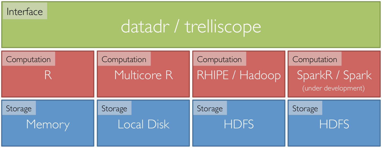
Tessera Environment
- Front end: two R packages, datadr & trelliscope
- Back ends: R, Hadoop, Spark, etc.
- R <-> backend bridges: RHIPE, SparkR, etc.
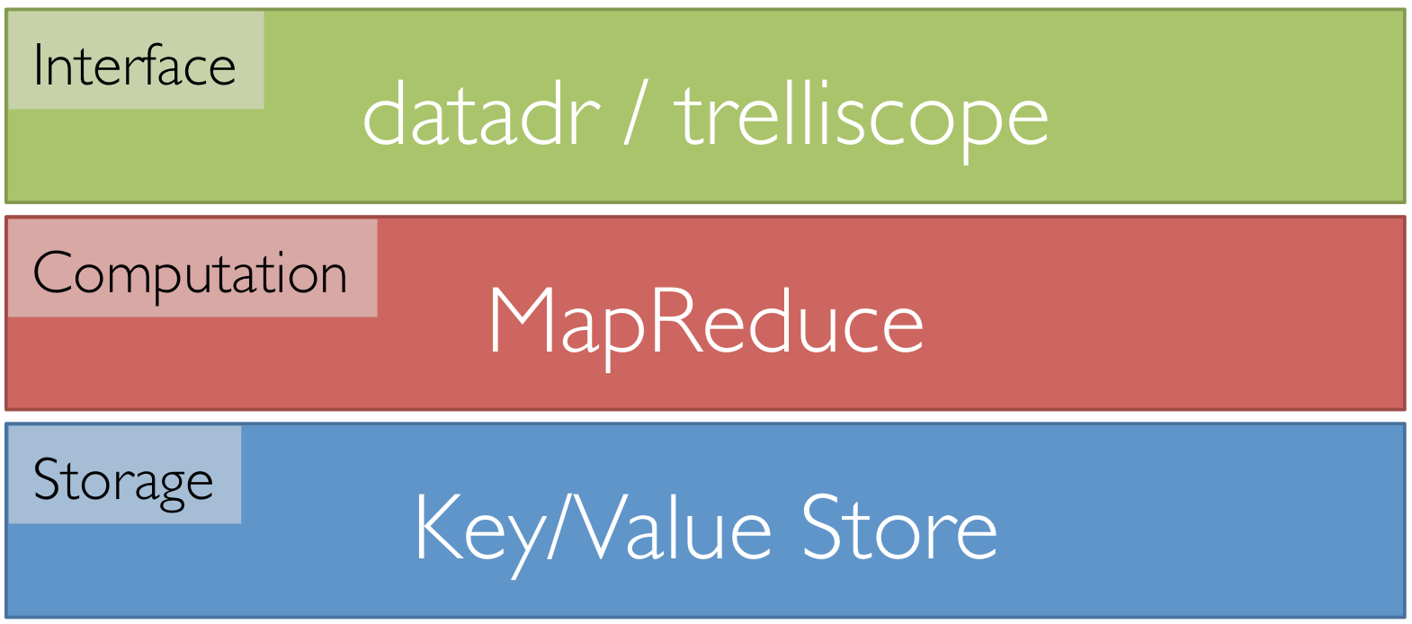
Back End Agnostic Interface
Trelliscope
-
Extension of multi-panel display systems, e.g. Trellis Display or faceting in ggplot
-
Number of panels can be very large (in the millions)
-
Panels can be interactively navigated through the use of cognostics
-
Provides flexible, scalable, detailed visualization of large, complex data

trelliscope example
Trelliscope is Scalable
- 6 months of high frequency trading data
- Hundreds of gigabytes of data
- Split by stock symbol and day
- Nearly 1 million subsets
Deep Analysis of
Large Complex Data
-
Data most often does not come with a model
-
If we already (think we) know the algorithm / model to apply and simply apply it to the data and do nothing else to assess validity, we are not doing analysis, we are processing
-
Deep analysis means detailed, comprehensive analysis that does not lose important information in the data
-
It means trial and error, an iterative process of hypothesizing, fitting, validating, learning
-
It means a lot of visualization
-
It means access to 1000s of statistical, machine learning, and visualization methods, regardless of data size
-
It means access to a high-level language to make iteration efficient
Deep Analysis of
Large Complex Data
Any or all of the following:
- Large number of records
- Many variables
- Complex data structures not readily put into tabular form of cases by variables
- Intricate patterns and dependencies that require complex models and methods of analysis
- Not i.i.d.!
Often complex data is more of a challenge than large data, but most large data sets are also complex
Goals
- Work in familiar high-level statistical programming environment
- Have access to the 1000s of statistical, ML, and vis methods
- Minimize time thinking about code or distributed systems
- Maximize time thinking about the data
- Be able to analyze large complex data with nearly as much flexibility and ease as small data
Divide and Recombine
- Specify meaningful, persistent divisions of the data
- Analytic or visual methods are applied independently to each subset of the divided data in embarrassingly parallel fashion
- Results are recombined to yield a statistically valid D&R result for the analytic method
Simple Idea
Divide and Recombine
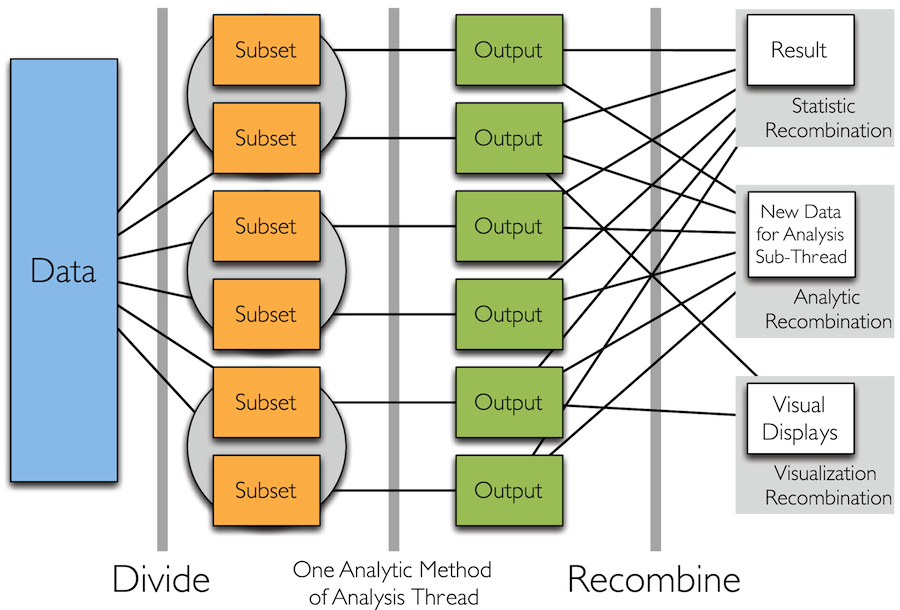
How to Divide the Data?
- Typically "big data" is big because it is made up of collections of smaller data from many subjects, sensors, locations, time periods, etc.
- It is therefore natural to break the data up based on these dimensions and apply visual or analytical methods to the subsets individually
- We call this conditioning variable division
- It is in practice by far the most common thing we do (and it's nothing new)
- Another option is random replicate division
Analytic Recombination
- Analytic recombination begins with applying an analytic method independently to each subset
- The beauty of this is that we can use any of the small-data methods we have available (think of the 1000s of methods in R)
- For conditioning-variable division:
- Typically the recombination depends on the subject matter
- Example: apply the same model to each subset and combine the subset estimated coefficients and build a statistical model or visually study the resulting collection of coefficients
Analytic Recombination
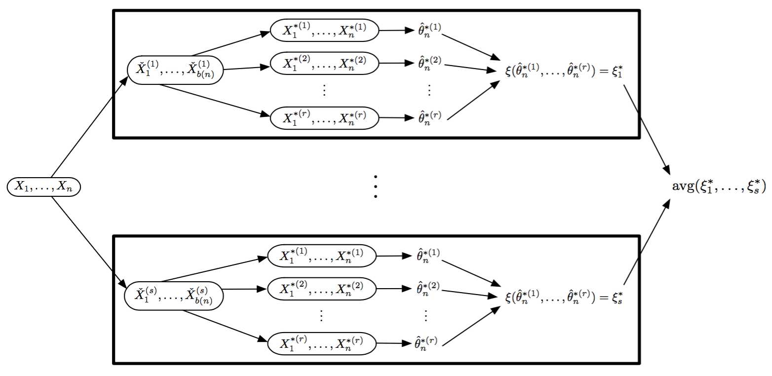
- For random replicate division:
- Observations are seen as exchangeable, with no conditioning variables considered
- Division methods are based on statistical matters, not the subject matter as in conditioning-variable division
- Results are often approximations
- Approaches that fit this paradigm
- Coefficient averaging
- Subset likelihood modeling
- Bag of little bootstraps
- Consensus MCMC
- Alternating direction method of multipliers (ADMM)
Visual Recombination: Trelliscope
-
Most tools and approaches for big data either
- Summarize lot of data and make a single plot
- Are very specialized for a particular domain
- Summaries are critical
- But we must be able to visualize complex data in detail even when they are large!
- Trelliscope does this by building on Trellis Display
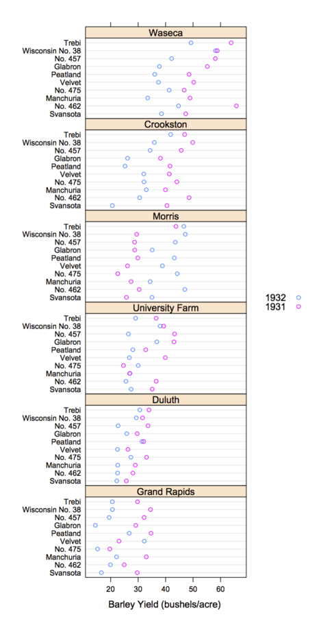
Trellis Display
- Data are split into meaningful subsets, usually conditioning on variables of the dataset
- A visualization method is applied to each subset
- The image for each subset is called a "panel"
- Panels are arranged in an array of rows, columns, and pages, resembling a garden trellis
Why Trellis is Effective
- Easy and effective to create
- Data complexity can be parametrized into how the data is split up and plotted
- We have a great deal of freedom with what we plot inside each panel
- Easy and effective to consume
- Edward Tufte’s term for panels in Trellis Display is
small multiples:
- Once a viewer understands one panel, they have immediate access to the data in all other panels
- Small multiples directly depict comparisons to reveal repetition and change, pattern and surprise
- Edward Tufte’s term for panels in Trellis Display is
small multiples:

Scaling Trellis
- Big data lends itself nicely to the idea of small multiples
- Typically "big data" is big because it is made up of collections of smaller data from many subjects, sensors, locations, time periods, etc.
- It is natural to break the data up based on these dimensions and plot it
- But this means Trellis displays with potentially thousands or millions of panels
- We can create millions of plots, but we will never be able to (or want to) view all of them!
Scaling Trellis
-
To scale, we can apply the same steps as in Trellis display, with one extra step:
- Data are split into meaningful subsets, usually conditioning on variables of the dataset
- A visualization method is applied to each subset
- A set of cognostic metrics is computed for each subset
- Panels are arranged in an array of rows, columns, and pages, resembling a garden trellis, with the arrangement being specified through interactions with the cognostics
We will see examples of creating Trelliscope displays in the following hands-on section
Tessera
Tessera is an implementation of D&R built on R
- Front end R packages that can tie to scalable back ends:
- datadr: provides an interface to data operations, division, and analytical recombination methods
- trelliscope: visual recombination through interactive multipanel exploration with cognostics

Data Structures in datadr
-
Must be able to break data down into pieces for independent storage / computation
-
Recall the potential for: “Complex data structures not readily put into tabular form of cases by variables”
-
Key-value pairs: a flexible storage paradigm for partitioned, distributed data
-
each subset of a division is an R list with two elements: key, value
-
keys and values can be any R object
-
[[1]]
$key
  [1] "setosa"

$value
  Sepal.Length Sepal.Width Petal.Length Petal.Width
           5.1         3.5          1.4         0.2
           4.9         3.0          1.4         0.2
           4.7         3.2          1.3         0.2
           4.6         3.1          1.5         0.2
           5.0         3.6          1.4         0.2
  ...


[[2]]
$key
  [1] "versicolor"

$value
   Sepal.Length Sepal.Width Petal.Length Petal.Width
            7.0         3.2          4.7         1.4
            6.4         3.2          4.5         1.5
            6.9         3.1          4.9         1.5
            5.5         2.3          4.0         1.3
            6.5         2.8          4.6         1.5
  ...

[[3]]
$key
  [1] "virginica"

$value
  Sepal.Length Sepal.Width Petal.Length Petal.Width
           6.3         3.3          6.0         2.5
           5.8         2.7          5.1         1.9
           7.1         3.0          5.9         2.1
           6.3         2.9          5.6         1.8
           6.5         3.0          5.8         2.2
  ...
Example: Fisher's iris data
We can represent the data divided by species as a collection of key-value pairs
- Key is species name
- Value is a data frame of measurements for that species
Measurements in centimeters of the variables sepal length and width and petal length and width for 50 flowers from each of 3 species of iris: "setosa", "versicolor", and "virginica"
Each key-value pair is an independent unit and can be stored across disks, machines, etc.
[[1]]
$key
  [1] "setosa"

$value
  Sepal.Length Sepal.Width Petal.Length Petal.Width
           5.1         3.5          1.4         0.2
           4.9         3.0          1.4         0.2
           4.7         3.2          1.3         0.2
           4.6         3.1          1.5         0.2
           5.0         3.6          1.4         0.2
  ...


[[2]]
$key
  [1] "versicolor"

$value
   Sepal.Length Sepal.Width Petal.Length Petal.Width
            7.0         3.2          4.7         1.4
            6.4         3.2          4.5         1.5
            6.9         3.1          4.9         1.5
            5.5         2.3          4.0         1.3
            6.5         2.8          4.6         1.5
  ...

[[3]]
$key
  [1] "virginica"

$value
  Sepal.Length Sepal.Width Petal.Length Petal.Width
           6.3         3.3          6.0         2.5
           5.8         2.7          5.1         1.9
           7.1         3.0          5.9         2.1
           6.3         2.9          5.6         1.8
           6.5         3.0          5.8         2.2
  ...
Distributed Data Objects &
Distributed Data Frames
A collection of key-value pairs that forms a data set is called a distributed data object (ddo) and is the fundamental data type that is passed to and returned from most of the functions in datadr.
A ddo for which every value in each key value pair is a data frame of the same schema is called a distributed data frame (ddf)
This is a ddf (and a ddo)
[[1]]
$key
  [1] "setosa"

$value
  Call:
  loess(formula = Sepal.Length ~ Sepal.Width, data = x)

  Number of Observations: 50
  Equivalent Number of Parameters: 5.53
  Residual Standard Error: 0.2437

[[2]]
$key
  [1] "versicolor"

$value
  Call:
  loess(formula = Sepal.Length ~ Sepal.Width, data = x)

  Number of Observations: 50
  Equivalent Number of Parameters: 5
  Residual Standard Error: 0.4483

[[3]]
$key
  [1] "virginica"

$value
  Call:
  loess(formula = Sepal.Length ~ Sepal.Width, data = x)

  Number of Observations: 50
  Equivalent Number of Parameters: 5.59
  Residual Standard Error: 0.5683
Distributed Data Objects &
Distributed Data Frames
Suppose we fit a loess model to each subset and store the result in a new collection of key-value pairs.
This is a ddo but not a ddf
datadr Data Connections
-
Distributed data types / backend connections
-
localDiskConn(), hdfsConn(), sparkDataConn() connections to ddo / ddf objects persisted on a backend storage system
-
ddo(): instantiate a ddo from a backend connection
-
ddf(): instantiate a ddf from a backend connection
-
-
Conversion methods between data stored on different backends
Computation in datadr
MapReduce
-
A general-purpose paradigm for processing big data sets
-
The standard processing paradigm in Hadoop
MapReduce
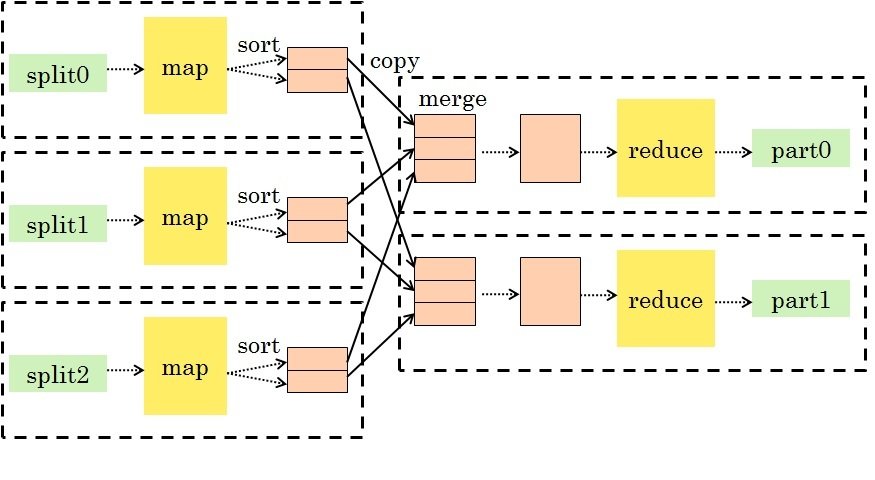
- Map: take input key-value pairs and apply a map function, emitting intermediate transformed key-value pairs
-
Shuffle: group map outputs by intermediate key
-
Reduce: for each unique intermediate key, gather all values and process with a reduce function

This is a very general and scalable approach to processing data.
MapReduce Example
- Map: for each species in the input key-value pair, emit the species as the key and the max as the value
- Reduce: for each grouped intermediate species key, compute the maximum of the values
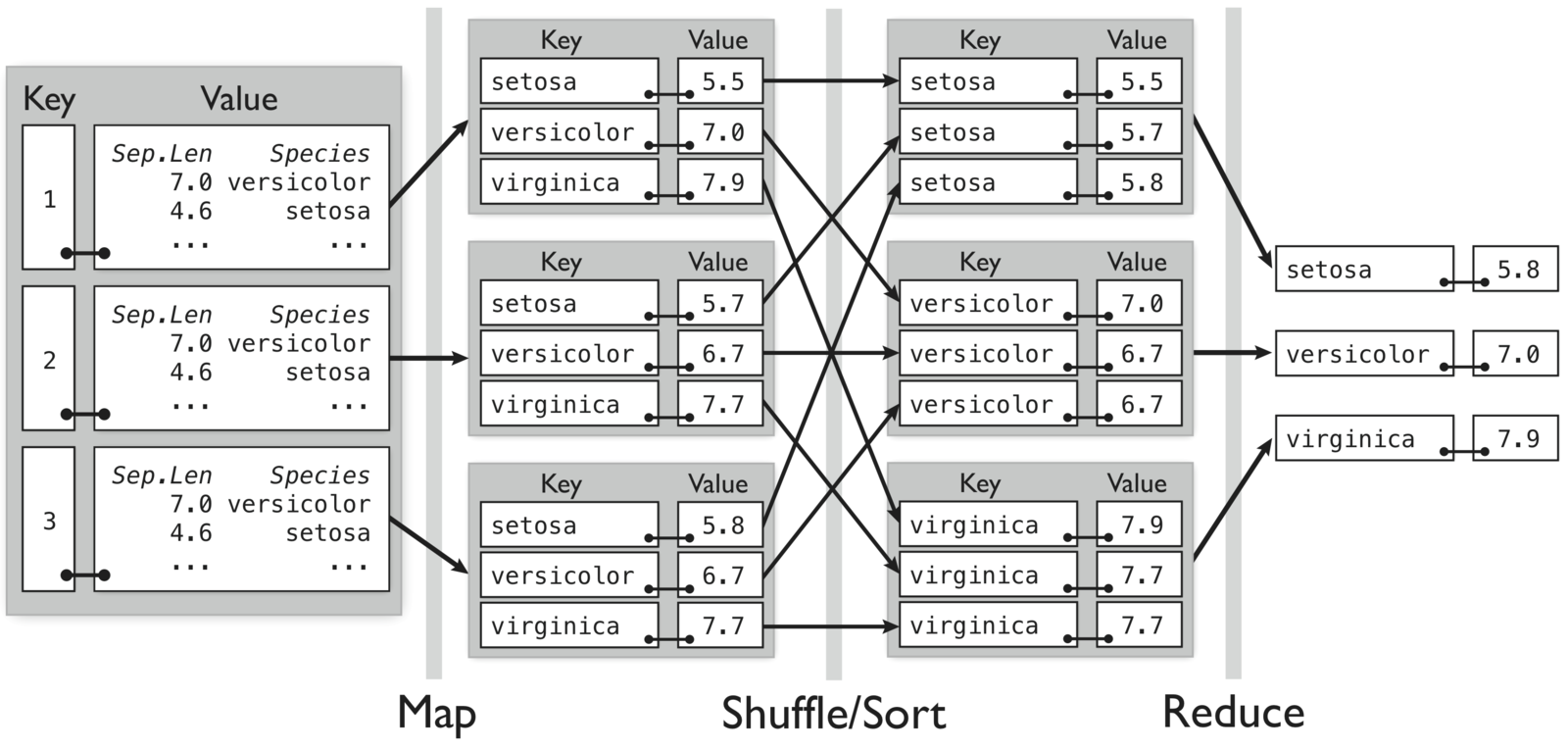
Compute maximum sepal length by species for randomly divided iris data
MapReduce Example
maxMap <- expression({
  # map.values: list of input values
  for(v in map.values) {
    # v is a data.frame
    # for each species, "collect" a
    # k/v pair to be sent to reduce
    by(v, v$Species, function(x) {
      collect(
        x$Species[1],       # key
        max(x$Sepal.Length) # value
      )
    })
  }
})
Map
# reduce is called for unique intermediate key
# "pre" is an initialization called once
# "reduce" is called for batches of reduce.values
# "post" runs after processing all reduce.values
maxReduce <- expression(
  pre={
    speciesMax <- NULL
  },
  reduce={
    curValues <- do.call(c, reduce.values)
    speciesMax <- max(c(speciesMax, curValues))
  },
  post={
    collect(reduce.key, speciesMax)
  }
)
Reduce
That's not very intuitive
But could be run on hundreds of terabytes of data
And it's much easier than what you'd write in Java
Computation in datadr
- Everything uses MapReduce under the hood
-
As often as possible, functions exist in datadr to shield the analyst from having to write MapReduce code
MapReduce is sufficient
for all D&R operations
D&R methods in datadr
-
A divide() function takes a ddf and splits it using conditioning or random replicate division
-
Analytic methods are applied to a ddo/ddf with the addTransform() function
-
Recombinations are specified with recombine(), which provides some standard combiner methods, such as combRbind(), which binds transformed results into single data frame
-
Division of ddos with arbitrary data structures must typically be done with custom MapReduce code (unless data can be temporarily transformed into a ddf)
datadr Other Data Operations
-
drLapply(): apply a function to each subset of a ddo/ddf and obtain a new ddo/ddf
-
drJoin(): join multiple ddo/ddf objects by key
-
drSample(): take a random sample of subsets of a ddo/ddf
-
drFilter(): filter out subsets of a ddo/ddf that do not meet a specified criteria
-
drSubset(): return a subset data frame of a ddf
-
drRead.table() and friends
-
mrExec(): run a traditional MapReduce job on a ddo/ddf
datadr Division Independent Methods
-
drQuantile(): estimate all-data quantiles, optionally by a grouping variable
-
drAggregate(): all-data tabulation
-
drHexbin(): all-data hexagonal binning aggregation
-
summary() method computes numerically stable moments, other summary stats (freq table, range, #NA, etc.)
-
More to come
datadr vs. dplyr
- dplyr
- "A fast, consistent tool for working with data frame like objects, both in memory and out of memory"
- Provides a simple interface for quickly performing a wide variety of operations on data frames
- Often datadr is confused as a dplyr alternative or competitor
- There are some similarities:
- Both are extensible interfaces for data anlaysis / manipulation
- Both have a flavor of split-apply-combine
datadr vs. dplyr
-
Back end architecture:
- dplyr ties to SQL-like back ends
- datadr ties to key-value stores
-
Scalability:
- At scale, dplyr is a glorified SQL wrapper (all computations must be translatable to SQL operations - no R code)
- datadr's fundamental algorithm is MapReduce, which scales to extremely large volumes and allows ad hoc R code to be applied
- Flexibility: dplyr data must be tabular while datadr data can be any conceivable R data structure
- Speed: dplyr will probably always be faster because its focused set of operations are optimized and usually applied against indexed databases whereas MapReduce always processes the entire data set
Differences
dplyr is great for subsetting, aggregating large tabular data
datadr is great for scalable deep analysis of large, complex data
For more information (docs, code, papers, user group, blog, etc.): http://tessera.io
Small Data Examples:
Home Prices from Zillow
Zillow Housing Data
- Housing sales and listing data in the United States
- Between 2008-10-01 and 2014-03-01
- Aggregated to the county level
- Zillow.com data provided by Quandl
library(housingData)

head(housing)

#    fips         county state       time nSold medListPriceSqft medSoldPriceSqft
# 1 06001 Alameda County    CA 2008-10-01    NA         307.9787         325.8118
# 2 06001 Alameda County    CA 2008-11-01    NA         299.1667               NA
# 3 06001 Alameda County    CA 2008-11-01    NA               NA         318.1150
# 4 06001 Alameda County    CA 2008-12-01    NA         289.8815         305.7878
# 5 06001 Alameda County    CA 2009-01-01    NA         288.5000         291.5977
# 6 06001 Alameda County CA 2009-02-01 NA 287.0370 NAHousing Data Variables
| Variable | Description |
|---|---|
| fips | Federal Information Processing Standard - a 5 digit county code |
| county | US county name |
| state | US state name |
| time | date (the data is aggregated monthly) |
| nSold | number sold this month |
| medListPriceSqft | median list price per square foot (USD) |
| medSoldPriceSqft | median sold price per square foot (USD) |
Data Ingest
- When working with any data set, the first thing to do is create a ddo/ddf from the data
- Examples:
## these are examples - don't run this code

# get data from a text file on HDFS and save to ddf on hdfs
myData1 <- drRead.table(
  hdfsConn("/home/input_text_files", header = TRUE, sep = "\t"),
  output = hdfsConn("/home/data_ddf")
)

# read from a csv file on disk and save ddf to disk
myData2 <- drRead.csv(
  localDiskConn("c:/my/local/data.csv"),
  output = localDiskConn("c:/my/local/data_ddf")
)

# convert in memory data frame to ddf:
myData3 <- ddf(some_data_frame)You Try It
Our housing data is already in memory, so we can use the simple approach of casting the data frame as a ddf:
library(datadr)
library(housingData)

housingDdf <- ddf(housing)
# print result to see what it looks like
housingDdf
# Distributed data frame backed by 'kvMemory' connection
#
# attribute | value
# ----------------+----------------------------------------------------------------
# names | fips(fac), county(fac), state(fac), time(Dat), and 3 more
# nrow | 224369
# size (stored) | 10.58 MB
# size (object) | 10.58 MB
# # subsets | 1
#
# * Other attributes: getKeys()
# * Missing attributes: splitSizeDistn, splitRowDistn, summaryDivide by county and state
One useful way to look at the data is divided by county and state
byCounty <- divide(housingDdf,
    by = c("county", "state"), update = TRUE)
* update = TRUE tells datadr to compute and update the attributes of the ddf (seen in printout)
byCounty

# Distributed data frame backed by 'kvMemory' connection
#
#  attribute      | value
# ----------------+----------------------------------------------------------------
#  names          | fips(cha), time(Dat), nSold(num), and 2 more
#  nrow           | 224369
#  size (stored)  | 15.73 MB
#  size (object)  | 15.73 MB
#  # subsets      | 2883
#
# * Other attributes: getKeys(), splitSizeDistn(), splitRowDistn(), summary()
# * Conditioning variables: county, stateInvestigating the ddf
Recall that a ddf is a collection of key-value pairs
# look at first key-value pair
byCounty[[1]]

# $key
# [1] "county=Abbeville County|state=SC"
#
# $value
#    fips       time nSold medListPriceSqft medSoldPriceSqft
# 1 45001 2008-10-01    NA         73.06226               NA
# 2 45001 2008-11-01    NA         70.71429               NA
# 3 45001 2008-12-01    NA         70.71429               NA
# 4 45001 2009-01-01    NA         73.43750               NA
# 5 45001 2009-02-01    NA         78.69565               NA
# ...
Investigating the ddf
# look at first two key-value pairs
byCounty[1:2]

# [[1]]
# $key
# [1] "county=Abbeville County|state=SC"#
#
# $value
#    fips       time nSold medListPriceSqft medSoldPriceSqft
# 1 45001 2008-10-01    NA         73.06226               NA
# 2 45001 2008-11-01    NA         70.71429               NA
# 3 45001 2008-12-01    NA         70.71429               NA
# 4 45001 2009-01-01    NA         73.43750               NA
# 5 45001 2009-02-01    NA         78.69565               NA
# ...#
#
#
# [[2]]
# $key
# [1] "county=Acadia Parish|state=LA"#
#
# $value
#    fips       time nSold medListPriceSqft medSoldPriceSqft
# 1 22001 2008-10-01    NA         67.77494               NA
# 2 22001 2008-11-01    NA         67.16418               NA
# 3 22001 2008-12-01    NA         63.59129               NA
# 4 22001 2009-01-01    NA         65.78947               NA
# 5 22001 2009-02-01    NA         65.78947               NA
# ...Investigating the ddf
# lookup by key
byCounty[["county=Benton County|state=WA"]]

# $key
# [1] "county=Benton County|state=WA"
#
# $value
#    fips       time nSold medListPriceSqft medSoldPriceSqft
# 1 53005 2008-10-01   137         106.6351         106.2179
# 2 53005 2008-11-01    80         106.9650               NA
# 3 53005 2008-11-01    NA               NA         105.2370
# 4 53005 2008-12-01    95         107.6642         105.6311
# 5 53005 2009-01-01    73         107.6868         105.8892
# ...You Try It
Try using the divide statement to divide on one or more variables
press down arrow key for solution when you're ready
Possible Solutions
byState <- divide(housing, by="state")

byMonth <- divide(housing, by="time")ddf Attributes
summary(byCounty)

#         fips                 time                nSold
#  -------------------  ------------------  -------------------
#        levels : 2883  missing :        0   missing :   164370
#       missing : 0         min : 08-10-01       min :       11
#  > freqTable head <       max : 14-03-01       max :    35619
#  26077 : 140                                  mean : 274.6582
#  51069 : 140                               std dev : 732.2429
#  08019 : 139                              skewness :   10.338
#  13311 : 139                              kurtosis : 222.8995
#  -------------------  ------------------  -------------------
# ...

names(byCounty)

# [1] "fips"             "time"             "nSold"            "medListPriceSqft"
# [5] "medSoldPriceSqft"

length(byCounty)

# [1] 2883

getKeys(byCounty)

# [[1]]
# [1] "county=Abbeville County|state=SC"
# ...Transformations
-
addTransform(data, fun) applies a function fun to each value of a key-value pair in the input ddo/ddf data
-
e.g. calculate a summary statistic for each subset
-
-
The transformation is not applied immediately, it is deferred until:
-
A function that kicks off a MapReduce job is called, e.g. recombine()
-
A subset of the data is requested (e.g. byCounty[[1]])
-
The drPersist() function explicitly forces transformation computation to persist
-
Transformation Example
Compute the slope of a simple linear regression of list price vs. time
# function to calculate a linear model and extract the slope parameter
lmCoef <- function(x) {
  coef(lm(medListPriceSqft ~ time, data = x))[2]
}

# best practice tip: test transformation function on one subset
lmCoef(byCounty[[1]]$value)

#          time
# -0.0002323686

# apply the transformation function to the ddf
byCountySlope <- addTransform(byCounty, lmCoef)Transformation example
# look at first key-value pair
byCountySlope[[1]]

# $key
# [1] "county=Abbeville County|state=SC"
#
# $value
#          time
# -0.0002323686

# what does this object look like?
byCountySlope

# Transformed distributed data object backed by 'kvMemory' connection
#
#  attribute      | value
# ----------------+----------------------------------------------------------------
#  size (stored)  | 15.73 MB (before transformation)
#  size (object)  | 15.73 MB (before transformation)
#  # subsets      | 2883
#
# * Other attributes: getKeys()
# * Conditioning variables: county, state
*note: this is a ddo (value isn't a data frame) but it is still pointing to byCounty's data
Exercise: create a transformation function
Create a new transformed data set using addTransform()
- Add/remove/modify variables
- Compute a summary (# rows, #NA, etc.)
- etc.
# get a subset
x <- byCounty[[1]]$value

# now experiment with x and stick resulting code into a transformation function

# some scaffolding for your solution:
transformFn <- function(x) {
  ## you fill in here
}

xformedData <- addTransform(byCounty, transformFn)
Hint: it is helpful to grab a subset and experiment with it and then stick that code into a function:
Possible Solutions
# example 1 - total sold over time for the county
totalSold <- function(x) {
   sum(x$nSold, na.rm=TRUE)
}
byCountySold <- addTransform(byCounty, totalSold)

# example 2 - range of time for which data exists for county
timeRange <- function(x) {
   range(x$time)
}
byCountyTime <- addTransform(byCounty, timeRange)

# example 3 - convert usd/sqft to aud/metre
us2aus <- function(x)
  x * 15.2453603

byCountyAus <- addTransform(byCounty, function(x) {
  x$medListPriceMetre <- us2aus(x$medListPriceSqft)
  x$medSoldPriceMetre <- us2aus(x$medSoldPriceSqft)
  x
})
Note that the us2aus function was detected - this becomes useful in distributed computing when shipping code across many computers
Recombination
countySlopes <- recombine(byCountySlope, combine = combRbind)
Let's recombine the slopes of list price vs. time into a data frame.
This is an example of statistic recombination where the result is small and is pulled back into R for further investigation.
head(countySlopes)

#           county state           val
# Abbeville County    SC -0.0002323686
#    Acadia Parish    LA  0.0019518441
#  Accomack County    VA -0.0092717711
#       Ada County    ID -0.0030197554
#     Adair County    IA -0.0308381951
# Adair County KY 0.0034399585Recombination Options
-
combine parameter controls the form of the result
-
combine=combRbind: rbind is used to combine all of the transformed key-value pairs into a local data frame in your R session - this is a frequently used option
-
combine=combCollect: transformed key-value pairs are collected into a local list in your R session
-
combine=combDdo: results are combined into a new ddo object
-
Others can be written for more sophisticated goals such as model coefficient averaging, etc.
-
Persisting a Transformation
us2aus <- function(x)
  x * 15.2453603

byCountyAus <- addTransform(byCounty, function(x) {
  x$medListPriceMetre <- us2aus(x$medListPriceSqft)
  x$medSoldPriceMetre <- us2aus(x$medSoldPriceSqft)
  x
})

byCountyAus <- drPersist(byCountyAus)
Often we want to persist a transformation, creating a new ddo or ddf that contains the transformed data. Transforming and persisting a transformation is an analytic recombination.
Let's persist our US to Australian transformation using drPersist():
*note we can also use recombine(combine = combDdf) - drPersist() is for convenience
Joining Multiple Datasets
We have a few additional data sets we'd like to join with our home price data divided by county
head(geoCounty)

#    fips         county state       lon      lat rMapState rMapCounty
# 1 01001 Autauga County    AL -86.64565 32.54009   alabama    autauga
# 2 01003 Baldwin County    AL -87.72627 30.73831   alabama    baldwin
# 3 01005 Barbour County    AL -85.39733 31.87403   alabama    barbour
# 4 01007    Bibb County    AL -87.12526 32.99902   alabama       bibb
# 5 01009  Blount County    AL -86.56271 33.99044   alabama     blount
# 6 01011 Bullock County    AL -85.71680 32.10634   alabama    bullock

head(wikiCounty)

#    fips         county state pop2013                                                 href
# 1 01001 Autauga County    AL   55246 http://en.wikipedia.org/wiki/Autauga_County,_Alabama
# 2 01003 Baldwin County    AL  195540 http://en.wikipedia.org/wiki/Baldwin_County,_Alabama
# 3 01005 Barbour County    AL   27076 http://en.wikipedia.org/wiki/Barbour_County,_Alabama
# 4 01007    Bibb County    AL   22512    http://en.wikipedia.org/wiki/Bibb_County,_Alabama
# 5 01009  Blount County    AL   57872  http://en.wikipedia.org/wiki/Blount_County,_Alabama
# 6 01011 Bullock County AL 10639 http://en.wikipedia.org/wiki/Bullock_County,_AlabamaExercise: Divide by County and State
- To join these with our byCounty data set, we first must divide them by county and state
- Give it a try:
byCountyGeo <- # ...

byCountyWiki <- # ...Exercise: Divide by County and State
byCountyGeo <- divide(geoCounty,
  by=c("county", "state"))

byCountyWiki <- divide(wikiCounty,
  by=c("county", "state"))
byCountyGeo
# Distributed data frame backed by 'kvMemory' connection
#
# attribute | value
# ----------------+----------------------------------------------------------------
# names | fips(cha), lon(num), lat(num), rMapState(cha), rMapCounty(cha)
# nrow | 3075
# size (stored) | 8.14 MB
# size (object) | 8.14 MB
# # subsets | 3075
# ...byCountyGeo[[1]]
# $key
# [1] "county=Abbeville County|state=SC"
#
# $value
# fips lon lat rMapState rMapCounty
# 1 45001 -82.45851 34.23021 south carolina abbevilleJoining the Data
drJoin() takes any number of named parameters specifying ddo/ddf objects and returns a ddo of the objects joined by key
joinedData <- drJoin(
  housing = byCountyAus,
  slope   = byCountySlope,
  geo     = byCountyGeo,
  wiki    = byCountyWiki)
joinedData
# Distributed data object backed by 'kvMemory' connection
#
# attribute | value
# ----------------+----------------------------------------------------------------
# size (stored) | 29.23 MB
# size (object) | 29.23 MB
# # subsets | 3144
Joining the Data
What does this object look like?
str(joinedData[[1]])

# List of 2
#  $ key  : chr "county=Abbeville County|state=SC"
#  $ value:List of 4
#   ..$ housing:'data.frame': 66 obs. of  7 variables:
#   .. ..$ fips             : chr [1:66] "45001" "45001" "45001" "45001" ...
#   .. ..$ time             : Date[1:66], format: "2008-10-01" "2008-11-01" ...
#   .. ..$ nSold            : num [1:66] NA NA NA NA NA NA NA NA NA NA ...
#   .. ..$ medListPriceSqft : num [1:66] 73.1 70.7 70.7 73.4 78.7 ...
#   .. ..$ medSoldPriceSqft : num [1:66] NA NA NA NA NA NA NA NA NA NA ...
#   .. ..$ medListPriceMetre: num [1:66] 1114 1078 1078 1120 1200 ...
#   .. ..$ medSoldPriceMetre: num [1:66] NA NA NA NA NA NA NA NA NA NA ...
#   ..$ slope  : Named num -0.000232
#   ..$ geo    :'data.frame': 1 obs. of  5 variables:
#   .. ..$ fips      : chr "45001"
#   .. ..$ lon       : num -82.5
#   .. ..$ lat       : num 34.2
#   .. ..$ rMapState : chr "south carolina"
#   .. ..$ rMapCounty: chr "abbeville"
#   ..$ wiki   :'data.frame': 1 obs. of  3 variables:
#   .. ..$ fips   : chr "45001"
#   .. ..$ pop2013: int 25007
#   .. ..$ href   : chr "http://en.wikipedia.org/wiki/Abbeville_County,_South Carolina"
# ...
for a given county/state, the value is a list with elements according to data provided in drJoin()
Joined Data
Note that joinedData has more subsets than byCountyAus
length(byCountyAus)

# [1] 2883

length(joinedData)

# [1] 3144- Some of the data sets we joined have more counties than we have data for in byCountyAus
- drJoin() makes a subset for every unique key across all input data sets
- If data is missing in a subset, it doesn't have an entry
# Adams County Iowa only has geo and wiki data
joinedData[["county=Adams County|state=IA"]]$value

# $geo
#    fips       lon      lat rMapState rMapCounty
# 1 19003 -94.70909 41.03166      iowa      adams
#
# $wiki
#    fips pop2013                                            href
# 1 19003 3894 http://en.wikipedia.org/wiki/Adams_County,_IowaBonus Problem
Can you write a transformation and recombination to get all counties for which joinedData does not have housing information?
Solution
noHousing <- joinedData %>%
  addTransform(function(x) is.null(x$housing)) %>%
  recombine(combRbind)

head(subset(noHousing, val == TRUE))

#               county state  val
# 2884    Adams County    IA TRUE
# 2885    Adams County    ND TRUE
# 2886 Antelope County    NE TRUE
# 2887   Arthur County    NE TRUE
# 2888   Ashley County    AR TRUE
# 2889   Aurora County    SD TRUE
tx <- addTransform(joinedData, function(x) is.null(x$housing))
noHousing <- recombine(tx, combRbind)(note about pipes)
Filtering
Suppose we only want to keep subsets of joinedData that have housing price data
- drFilter(data, fun) applies a function fun to each value of a key-value pair in the input ddo/ddf data
- If fun returns TRUE we keep the key-value pair
joinedData <- drFilter(joinedData,
  function(x) {
    !is.null(x$housing)
  })
# joinedData should now have as many subsets as byCountyAus
length(joinedData)
# [1] 2883Trelliscope
- We now have a ddo, joinedData, which contains pricing data as well as a few other pieces of information like geographic location and a link to wikipedia for 2,883 counties in the US
- Using this data, let's make a simple plot of list price vs. time for each county and put it in a Trelliscope display
Trelliscope Setup
- Trelliscope stores its displays in a "Visualization Database" (VDB), which is a collection of files on your disk that contain metadata about the displays
- To create and view displays, we must first establish a connection to the VDB
library(trelliscope)

# establish a connection to a VDB located in a directory "housing_vdb"
vdbConn("housing_vdb", name = "shortcourse")- If this location has not already been initialized as a VDB, you will be prompted if you want to create one at this location (you can set autoYes = TRUE to skip the prompt)
- If it has been initialized, it will simply make the connection
Trelliscope Display Fundamentals
- A Trelliscope display is created with the function makeDisplay()
- At a minimum, a specification of a Trelliscope display must have the following:
- data: a ddo or ddf input data set
- name: the name of the display
- panelFn: a function that operates on the value of each key-value pair and produces a plot
- There are several other options, some of which we will see and some of which you can learn more about in the documentation
A Simple Panel Function
Plot list price vs. time using rbokeh
library(rbokeh)

timePanel <- function(x) {
  xlim <- c("2008-07-01", "2014-06-01")

  figure(ylab = "Price / Sq. Metre (AUD)",
    xlim = as.Date(xlim)) %>%
  ly_points(time, medListPriceMetre,
    data = x$housing,
    hover = list(time, medListPriceMetre))
}

# test it on a subset
timePanel(joinedData[[1]]$value)Make a Display
makeDisplay(joinedData,
  name = "list_vs_time_rbokeh",
  desc = "List price over time for each county.",
  panelFn = timePanel
)
- This creates a display and adds its meta data to the directory we specified in vdbConn()
- We can view the display with this:
view()

# to go directly to this display
view("list_vs_time_rbokeh")Try Your Own Panel Function
Ideas: recreate the previous plot with your favorite plotting package, or try something new (histogram of prices, etc.)
Make a panel function,
test it,
and make a new display with it
Possible Solutions
library(lattice)
library(ggplot2)

latticeTimePanel <- function(x) {
  xyplot(medListPriceMetre + medSoldPriceMetre ~ time,
    data = x$housing, auto.key = TRUE,
    ylab = "Price / Metre (AUD)")
}

makeDisplay(joinedData,
  name = "list_vs_time_lattice",
  desc = "List price over time for each county.",
  panelFn = latticeTimePanel
)

ggTimePanel <- function(x) {
  qplot(time, medListPriceMetre, data = x$housing,
    ylab = "Price / Metre (AUD)") +
  geom_point()
}

makeDisplay(joinedData,
  name = "list_vs_time_ggplot2",
  desc = "List price over time for each county.",
  panelFn = ggTimePanel
)A Display with Cognostics
- The interactivity in these examples hasn't been too interesting
- We can add more interactivity through cognostics
- Like the panel function, we can supply a cognostics function that
- Takes a subset of the data as input and returns a named list of summary statistics or cognostics about the subset
- A helper function cog() can be used to supply additional attributes like descriptions to help the viewer understand what the cognostic is
- These can be used for enhanced interaction with the display, helping the user focus their attention on panels of interest
Cognostics Function
zillowCog <- function(x) {
  # build a string for a link to zillow
  st <- getSplitVar(x, "state")
  ct <- getSplitVar(x, "county")
  zillowString <- gsub(" ", "-", paste(ct, st))

  # return a list of cognostics
  list(
    slope = cog(x$slope, desc = "list price slope"),
    meanList = cogMean(x$housing$medListPriceMetre),
    meanSold = cogMean(x$housing$medSoldPriceMetre),
    lat = cog(x$geo$lat, desc = "county latitude"),
    lon = cog(x$geo$lon, desc = "county longitude"),
    wikiHref = cogHref(x$wiki$href, desc="wiki link"),
    zillowHref = cogHref(
      sprintf("http://www.zillow.com/homes/%s_rb/", zillowString),
      desc="zillow link")
  )
}
# test it on a subset
zillowCog(joinedData[[1]]$value)
# $slope
# time
# -0.0002323686
#
# $meanList
# [1] 1109.394
#
# $meanSold
# [1] NaN
#
# $lat
# [1] 34.23021
#
# $lon
# [1] -82.45851
#
# $wikiHref
# [1] "<a href=\"http://en.wikipedia.org/wiki/Abbeville_County,_South Carolina\" target=\"_blank\">link</a>"
#
# $zillowHref
# [1] "<a href=\"http://www.zillow.com/homes/Abbeville-County-SC_rb/\" target=\"_blank\">link</a>"
Display with Cognostics
We simply add our cognostics function to makeDisplay()
makeDisplay(joinedData,
  name = "list_vs_time_cog",
  desc = "List price over time for each county.",
  panelFn = timePanel,
  cogFn = zillowCog
)Medium Data Examples:
NYC Taxi Data
NYC Taxi Data
- Taxi ride data for NYC for 2013 (data source)
- 173,179,759 rides
- 30 GB raw text csv files
- A subset of 1M rides in Manhattan has been provided:
read.csv("taxidata/raw_csv/taxi.csv", nrows = 3)

#   medal hack vendor ratelevel flag        pickdatetime        dropdatetime
# 1   hkm bvca    VTS         1      2013-04-07 08:43:00 2013-04-07 08:47:00
# 2   vso vxga    VTS         1      2013-09-21 00:08:00 2013-09-21 00:32:00
# 3   nho ukvb    CMT         1    N 2013-04-30 02:10:34 2013-04-30 02:13:21
#   passnum ridetimemet ridedis  picklong  picklat  droplong  droplat paytype
# 1       1         240    1.04 -74.00241 40.74785 -73.99725 40.73743     CSH
# 2       3        1440    6.69 -74.00109 40.73394 -73.96391 40.80785     CRD
# 3       1         166    0.70 -73.97559 40.74529 -73.97772 40.75217     CRD
#   meter surcharge tax  tip toll  fare ridetime pickregion   dropregion
# 1   5.0       0.0 0.5 0.00    0  5.50      240       man4         man2
# 2  24.0       0.5 0.5 3.50    0 28.50     1440       man2         man9
# 3 4.5 0.5 0.5 1.37 0 6.87 167 man6 GrandCentral| medal | yellow-cab medallion ID (obfuscated) |
| hack | driver's yellow cab license ID (obfuscated) |
| vendor | cab communication system |
| ratelevel | taximeter rate charging type |
| flag | unknown |
| pickdatetime | pick-up time of the ride |
| dropdatetime | drop-off time of the ride |
| passnum | number of passengers |
| ridetimemet | ride time measured by the taximeter in seconds |
| ridedis | ride distance measured by the taximeter in miles |
| picklong | longitude of the pick-up location |
| picklat | latitude of the pick-up location |
| droplong | longitude of the drop-off location |
| droplat | latitude of the drop-off location |
| paytype | payment type: "CRD" "CSH" "DIS" "NOC" "UNK" |
| meter | fare showing on meter in USD |
| surcharge | extra fees in USD |
| tax | tax in USD |
| tip | tip in USD |
| toll | tolls in USD |
| fare | total charge in USD |
| ridetime | ride time - drop-off time minus pick-up time, in seconds |
| pickregion | pick-up region |
| dropregion | drop-off region |
Taxi Variables
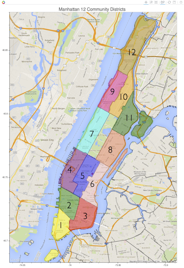
Manhattan Regions
The pick up and drop off locations have been categorized into 12 districts plus three "hot spots" - Penn Station, Grand Central Station, and Central Park
Taxi Data Examples
- We are only looking at a small subset of the data
- Logistical issues with all students analyzing all 30 GB on a cluster
- You can use your laptop for these examples
- This subset is small enough to deal with in memory
- But we will use the intermediate storage / compute option, "local disk", to illustrate the step up from in-memory
- Once you understand this step up, using Hadoop as the back-end is straightforward
- We will illustrate using Hadoop on all of the data at the end of the day
Taxi Data Analysis Goals
- Exploratory data analysis
- Try to understand the variables in the data and their distributions / relationships
- This will simulate a more practical example of what we deal with in real-world situations
- Open-ended:
- We will show several examples and provide some guided questions to allow some freedom of exploration
- A lot of emphasis will be placed on division-agnostic methods (quantiles, aggregation, etc.), which we didn't cover in the housing example
Taxi Data: Environment Setup
Load packages and set up local "cluster"
# make sure you have set your working directory correctly
list.files()

# [1] "housing.R" "taxi.R"    "taxidata"

library(datadr)
library(trelliscope)
library(parallel)
library(lubridate)
library(rbokeh)

# set the default backend to be R multicore with 4 cores
# feel free to replace 4 with 1,2,3
options(defaultLocalDiskControl = localDiskControl(makeCluster(4)))
Read in Raw Data
# this steps through blocks of the input file (serially)
# and creates a ddf with one subset for each block
raw <- drRead.csv("taxidata/raw_csv/taxi.csv",
  output = localDiskConn("taxidata/raw"))

raw

# Distributed data frame backed by 'kvLocalDisk' connection

#  attribute      | value
# ----------------+----------------------------------------------------------------
#  names          | medal(cha), hack(cha), vendor(cha), ratelevel(int), and 20 more
#  nrow           | [empty] call updateAttributes(dat) to get this value
#  size (stored)  | 41.89 MB
#  size (object)  | [empty] call updateAttributes(dat) to get this value
#  # subsets      | 20

# * Missing attributes: keys, splitSizeDistn, splitRowDistn, summary
- Raw csv file is located in "taxidata/raw_csv/taxi.csv"
- We can use drRead.csv() to read this in as a ddf
- Note that we must specify a place to store the output, using localDiskConn()
Local Disk Connections
list.files("taxidata/raw")

#  [1] "_meta"
#  [2] "0aee9b78301d7ec8998971363be87c03.Rdata"
#  [3] "1937e7b7bc06d5dc1531976d1c355670.Rdata"
#  [4] "23c80a31c0713176016e6e18d76a5f31.Rdata"
#  [5] "2522027d230e3dfe02d8b6eba1fd73e1.Rdata"
#  [6] "30986e242495ba4a216a86700f7ece29.Rdata"
#  [7] "3f880ddf0d5f56067f2833ad76b3b226.Rdata"
#  [8] "4a5d7d50676e6d0ea065f445d8a5539d.Rdata"
#  [9] "5511291e2e560122bcb2e3261d58e289.Rdata"
# [10] "5e338704a8e069ebd8b38ca71991cf94.Rdata"
# [11] "6717f2823d3202449301145073ab8719.Rdata"
# [12] "709a7faa72cb6f3be79d683e234ccb25.Rdata"
# [13] "7260985235f3e5b1cd7097b1c768c19a.Rdata"
# [14] "90a7653d717dc1553ee564aa27b749b9.Rdata"
# [15] "a86d0670df7fb4f1da7b38943f5ee4e7.Rdata"
# [16] "c72d0198505540505acfb4b2b49911e6.Rdata"
# [17] "c8f1af0c7b420d99059a2c8d079c51bf.Rdata"
# [18] "db8e490a925a60e62212cefc7674ca02.Rdata"
# [19] "dbc09cba9fe2583fb01d63c70e1555a8.Rdata"
# [20] "e5b57f323c7b3719bbaaf9f96b260d39.Rdata"
# [21] "e8c6c490beabf8e7ab89dcd59a75f389.Rdata"
- We specified the output using localDiskConn()
- This specifies a connection to ddo/ddf key-value pairs stored on your local hard drive
- If the connection is for output, it is typically a connection to an empty directory
- Each subset key/value pair is stored as a file in this directory
- When working in local disk mode, all inputs and outputs to datadr operations can be local disk connections
Local Disk Connection Persistence
raw <- ddf(localDiskConn("taxidata/raw"))

# make sure it still looks the same
raw

# Distributed data frame backed by 'kvLocalDisk' connection

#  attribute      | value
# ----------------+----------------------------------------------------------------
#  names          | medal(cha), hack(cha), vendor(cha), ratelevel(int), and 20 more
#  nrow           | [empty] call updateAttributes(dat) to get this value
#  size (stored)  | 41.89 MB
#  size (object)  | [empty] call updateAttributes(dat) to get this value
#  # subsets      | 20

# * Missing attributes: keys, splitSizeDistn, splitRowDistn, summary
- If we leave our R session and want to come back to our analysis later, we want our previous work to persist
-
We can establish a ddo/ddf that points to data on a local disk connection, for example our ddf located in "taxidata/raw", with the following:
Local Disk ddo/ddf Objects
str(raw[[1]])

# List of 2
#  $ key  : num 6
#  $ value:'data.frame':  50000 obs. of  24 variables:
#   ..$ medal       : chr [1:50000] "nae" "tal" "ehi" "kpe" ...
#   ..$ hack        : chr [1:50000] "badc" "erua" "lqva" "lbhb" ...
#   ..$ vendor      : chr [1:50000] "CMT" "CMT" "VTS" "CMT" ...
#   ..$ ratelevel   : int [1:50000] 1 1 1 1 1 1 1 1 1 1 ...
#   ..$ flag        : chr [1:50000] "N" "N" "" "N" ...
#   ..$ pickdatetime: chr [1:50000] "2013-05-12 22:58:32" "2013-05-08 13:41:10" "2013-05-07 22:13:00" "2013-02-08 09:52:33" ...
#   ..$ dropdatetime: chr [1:50000] "2013-05-12 23:08:05" "2013-05-08 13:50:26" "2013-05-07 22:16:00" "2013-02-08 10:03:19" ...
#   ..$ passnum     : int [1:50000] 1 2 1 1 1 1 1 6 1 3 ...
#   ..$ ridetimemet : int [1:50000] 271 556 180 646 840 1080 493 120 300 1020 ...
#   ..$ ridedis     : num [1:50000] 1 1.3 0.85 2 3.4 1.54 0.9 0.05 1.15 6.28 ...
#   ..$ picklong    : num [1:50000] -74 -74 -74 -74 -74 ...
#   ..$ picklat     : num [1:50000] 40.8 40.8 40.7 40.8 40.7 ...
#   ..$ droplong    : num [1:50000] -74 -74 -74 -74 -74 ...
#   ..$ droplat     : num [1:50000] 40.8 40.7 40.7 40.7 40.8 ...
#   ..$ paytype     : chr [1:50000] "CRD" "CRD" "CSH" "CRD" ...
#   ..$ meter       : num [1:50000] 5.5 8 4.5 9.5 13 12 7 3.5 6 19.5 ...
#   ..$ surcharge   : num [1:50000] 0.5 0 0.5 0 0.5 0 0 0.5 0 0.5 ...
#   ..$ tax         : num [1:50000] 0.5 0.5 0.5 0.5 0.5 0.5 0.5 0.5 0.5 0.5 ...
#   ..$ tip         : num [1:50000] 1.3 1.7 0 2 2 2 0 0 1.2 0 ...
#   ..$ toll        : num [1:50000] 0 0 0 0 0 0 0 0 0 0 ...
#   ..$ fare        : num [1:50000] 7.8 10.2 5.5 12 16 14.5 7.5 4.5 7.7 20.5 ...
#   ..$ ridetime    : int [1:50000] 573 556 180 646 840 1080 493 120 300 1020 ...
#   ..$ pickregion  : chr [1:50000] "GrandCentral" "man4" "man3" "PennStation" ...
# ..$ dropregion : chr [1:50000] "PennStation" "man5" "man6" "man3" ...- ddo/ddf objects stored on local disk behave in exactly the same way a we saw for in-memory
- For example, accessing subsets of the data:
* note: keys were assigned by drRead.csv() to be 1, 2, ...
Local Disk ddo/ddf Objects
nrow(raw)

# [1] NA
# Warning message:
# In nrow(raw) :
#   Number of rows has not been computed - run updateAttributes on this object
However, note that not all attributes are available:
- This is due to the fact that when given a large out-of-memory set of data, there are some attributes we cannot know (like total number of rows) until computing over the entire data set
- This isn't as much of an issue with in-memory data because a pass over the data is easy
- We can explicitly ask for these attributes to be computed with updateAttributes()
Updating Attributes
raw <- updateAttributes(raw)

raw

# Distributed data frame backed by 'kvLocalDisk' connection

#  attribute      | value
# ----------------+----------------------------------------------------------------
#  names          | medal(cha), hack(cha), vendor(cha), ratelevel(int), and 20 more
#  nrow           | 1000000
#  size (stored)  | 41.89 MB
#  size (object)  | 337.85 MB
#  # subsets      | 20

# * Other attributes: getKeys(), splitSizeDistn(), splitRowDistn(), summary()

nrow(raw)

# [1] 1000000
However, note that not all attributes are available:
Exploration: Summaries
summary(raw)

#         medal                  hack                 vendor
# ---------------------  ---------------------  ------------------
#       levels : 10000+        levels : 10000+        levels : 2
#      missing : 0            missing : 0            missing : 0
#  > freqTable head <     > freqTable head <    > freqTable head <
# fah : 163              ogtb : 109             VTS : 500811
# jyr : 157              vssa : 106             CMT : 499189
# rfp : 154              qdia : 102
# iet : 153              rwxb : 102
# ---------------------  ---------------------  ------------------
#      ratelevel               flag              pickdatetime
# --------------------  ------------------  -----------------------
#  missing :         0        levels : 3          levels : 10000+
#      min :         0       missing : 0         missing : 0
#      max :         6  > freqTable head <    > freqTable head <
#     mean :  1.003798    : 500946          2013-02-12 09:19:00 : 9
#  std dev : 0.1100981  N : 487911          2013-03-02 18:55:00 : 9
# skewness :  30.84596  Y :  11143          2013-03-06 07:37:00 : 9
# kurtosis :  1035.261                      2013-04-24 08:23:00 : 9
# --------------------  ------------------  -----------------------
#       dropdatetime              passnum            ridetimemet
# ------------------------  -------------------  -------------------
#       levels : 10000+      missing :        0   missing :        0
#      missing : 0               min :        1       min :      -10
#    > freqTable head <          max :        6       max :  4294739
# 2013-01-26 22:23:00 : 10      mean : 1.707755      mean : 741.4466
# 2013-01-25 22:27:00 :  9   std dev : 1.377656   std dev : 17647.23
# 2013-03-05 18:53:00 :  9  skewness : 2.016229  skewness :  242.322
# 2013-04-03 22:16:00 :  9  kurtosis : 5.836064  kurtosis : 58757.79
# ------------------------  -------------------  -------------------
#       ridedis              picklong                picklat
# -------------------  ---------------------  ---------------------
#  missing :        0   missing :          0   missing :          0
#      min :        0       min :  -74.02251       min :   40.68776
#      max :   250000       max :  -73.91147       max :   40.87636
#     mean : 2.434937      mean :  -73.98106      mean :   40.75546
#  std dev : 250.0045   std dev : 0.01697669   std dev : 0.02392806
# skewness : 999.9183  skewness :  0.3124089  skewness :  0.5125662
# kurtosis :   999891  kurtosis :   2.591296  kurtosis :   3.927271
# -------------------  ---------------------  ---------------------
#       droplong                droplat              paytype
# ---------------------  ---------------------  ------------------
#  missing :          0   missing :          0        levels : 5
#      min :  -74.01847       min :    40.7009       missing : 0
#      max :  -73.91145       max :   40.87631  > freqTable head <
#     mean :  -73.98015      mean :   40.75685  CRD : 533697
#  std dev : 0.01782197   std dev : 0.02586537  CSH : 462464
# skewness :  0.3684803  skewness :  0.7079717  NOC :   2030
# kurtosis :   2.725493  kurtosis :   4.416856  UNK :   1151
# ---------------------  ---------------------  ------------------
#        meter              surcharge                 tax
# -------------------  --------------------  ---------------------
#  missing :        0   missing :         0   missing :          0
#      min :       -5       min :        -1       min :       -0.5
#      max :      353       max :         7       max :        0.5
#     mean : 10.29182      mean : 0.3180572      mean :  0.4997165
#  std dev : 5.739544   std dev : 0.3656158   std dev : 0.01219302
# skewness : 2.641248  skewness : 0.6997366  skewness :  -44.82106
# kurtosis :  43.3373  kurtosis :  2.413585  kurtosis :   2153.374
# -------------------  --------------------  ---------------------
#         tip                  toll                  fare
# -------------------  ---------------------  -------------------
#  missing :        0   missing :          0   missing :        0
#      min :        0       min :          0       min :       -6
#      max :      150       max :      40.75       max :      403
#     mean : 1.097984      mean : 0.00499029      mean : 12.21265
#  std dev : 1.489039   std dev :  0.1787053   std dev : 6.521503
# skewness : 8.299564  skewness :   48.87434  skewness : 2.666064
# kurtosis : 472.5249  kurtosis :   4429.004  kurtosis : 41.10018
# -------------------  ---------------------  -------------------
#      ridetime            pickregion          dropregion
# -------------------  ------------------  ------------------
#  missing :        0        levels : 15         levels : 15
#      min :    -3100       missing : 0         missing : 0
#      max :    16213  > freqTable head <  > freqTable head <
#     mean : 669.5678  man5 : 216790       man5 : 223404
#  std dev : 435.7753  man8 : 150980       man8 : 146494
# skewness : 2.055302  man6 : 115442       man6 : 110488
# kurtosis : 19.57769  man4 : 107727       man4 : 105844
# -------------------  ------------------  ------------------
A good place to start is to look at the variable summaries (provided by updateAttributes)
Summary Observations
- No missing values
- Negative values for things that should intuitively be non-negative
-
Hack and mediallian have 10k+ levels
- for computational efficiency, only 10k levels are computed for summaries but we can get more detail with other functions
- Note: ratelevel is treated as numeric but we'd like it to be categorical
-
Note: datetimes are categorical bue we'd like them to be categorical
- We can fix these in our initial read-in by specifying colClasses
- Or we can fix this later with a transformation
- Note: summaries are scalable and computed with MapReduce (so we can get these on terabytes of data) and the algorithms are numerically stable
Exploration: Summaries
pickft <- summary(raw)$pickregion$freqTable

head(pickft)

#    value   Freq
# 10  man5 216790
# 13  man8 150980
# 11  man6 115442
# 9   man4 107727
# 7   man2 105491
# 12  man7  93193

figure(ylim = rev(pickft$value),
  ylab = NULL) %>%
  ly_points(Freq, value,
    data = pickft, hover = pickft)
We can extract data from the summaries
Exploration: Summaries
pick <- summary(raw)$pickregion$freqTable
drop <- summary(raw)$dropregion$freqTable
both <- make.groups(pick = pick, drop = drop)

figure() %>%
  ly_bar(value, Freq, color = which,
    data = both, position = "dodge") %>%
  theme_axis("x",
    major_label_orientation = 90)
Pick up and drop off distributions
Exploration: Summaries
Pick a categorical variable and make a plot of its frequency distribution
Pick a quantitative variable and inspect its summary contents
Possible Solutions
# hack frequency table
hft <- summary(raw)$hack$freqTable

plot(sort(hft$Freq),
  ylab = "Hack frequency (top/bottom 5000)")


summary(raw)$tip

# $nna
# [1] 0

# $stats
# $stats$mean
# [1] 1.097984

# $stats$var
# [1] 2.217236

# $stats$skewness
# [1] 8.299564

# $stats$kurtosis
# [1] 472.5249

# $range
# [1]   0 150
Exploration: Quantiles
- We were able to use the summary data to explore distributions of categorical variables
- But what about continuous variables?
- We can use drQuantile() to estimate the quantiles of a continuous variable
- Note that the results of drQuantile() are approximate
- drQuantile() uses a scalable algorithm that slices the range of the variable up into small bins, tabulates counts within the bins, and transforms the result into approximate quantiles
- Thus we can compute distributions on extremely large data sets
Exploration: Quantiles
pc_quant <- drQuantile(raw,
  var = "passnum", tails = 1)

head(pc_quant)

#    fval q
# 1 0.000 1
# 2 0.005 1
# 3 0.010 1
# 4 0.015 1
# 5 0.020 1
# 6 0.025 1

figure() %>%
  ly_points(fval, q, data = pc_quant)
Compute the distrubution of the number of passengers
Over 70% of rides in Manhattan have a single passenger, etc.
Exploration: Quantiles
Compute and plot the distribution of ridetime
Solution
rt_quant <- drQuantile(raw,
  var = "ridetime", tails = 1)

figure(ylab = "ride time (minutes)") %>%
 ly_points(fval, q / 60, data = rt_quant)
Quantiles with Transformations
- Sometimes we want to transform a variable prior to its quantile computation
- We can do this by providing a function to varTransFn in drQuantile()
- For example, ride distance has a very large range and perhaps we want its distribution on the log scale:
summary(raw)$ridedis$range
# [1]      0 250000

# a ride distance of 250k miles!
# do a log + 1 transformation
rd_quant <- drQuantile(raw,
  var = "ridedis", tails = 1,
  varTransFn = function(x) log10(x + 1))

figure(ylab = "ride distance log10(miles + 1)") %>%
ly_points(fval, q, data = rd_quant,
  hover = rd_quant)
* note: it's a good idea to look at the range of a variable prior to computing its distribution
Quantiles with Conditioning
- It is useful to be able to compute distributions conditioned on some variable
- We can do this by specifying by in drQuantile()
- For example, let's look at the distribution of tip amount by payment type:
tip_quant <- drQuantile(raw, var = "tip",
  by = "paytype", tails = 1,
  probs = seq(0, 1, 0.05))

head(tip_quant)

#   fval         q paytype
# 1 0.00 0.0000000     CRD
# 2 0.05 0.7950795     CRD
# 3 0.10 1.0051005     CRD
# 4 0.15 1.0051005     CRD
# 5 0.20 1.0051005     CRD
# 6 0.25 1.0951095     CRD

figure(ylab = "tip amount (USD)",
  legend_location = "top_left") %>%
  ly_points(fval, q, color = paytype,
    data = subset(tip_quant, q < 100))
Exploration: Hexbin
- A useful way to visualize bivariate relationships with lots of data is using a hexbin plot - partitioning into a grid of hexagons and counting x/y frequency
- This is simple to scale, and is available through drHexbin()
- For example, let's look at latitude vs. longitude:
pickup_latlon <- drHexbin("picklong", "picklat",
  data = raw, xbins = 300, shape = 1.7)

hexbin::plot(pickup_latlon,
  trans = log, inv = exp,
  style = "colorscale",
  xlab = "longitude", ylab = "latitude",
  colramp = hexbin::LinOCS)
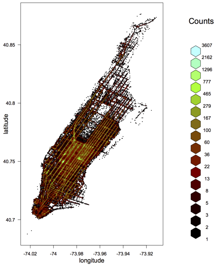
Dealing with Bad Data
- We've noticed a few issues with the data so far
- Let's take a closer look at some of these records
# get all records that went more than 100 miles
# or have negative ride time or fare
bad <- drSubset(raw, ridedis > 100 | ridetime < 0 | fare < 0)

head(bad)

#   medal hack vendor ratelevel flag        pickdatetime        dropdatetime
# 1   tad bupa    VTS         1      2013-08-25 14:47:10 2013-08-25 14:51:00
# 2   rbb qjyb    VTS         1      2013-08-07 11:52:10 2013-08-07 11:55:00
# 3   aaq xyna    VTS         1      2013-08-08 05:33:10 2013-08-08 05:37:00
# 4   ofs hlka    VTS         1      2013-08-21 01:04:10 2013-08-21 01:06:00
# 5   jzq eiub    CMT         1    N 2013-03-10 03:51:52 2013-03-10 03:00:12
# 6   yij hdab    VTS         1      2013-08-14 20:23:10 2013-08-14 20:27:00
#   passnum ridetimemet ridedis  picklong  picklat  droplong  droplat paytype
# 1       1         230    0.50 -73.97270 40.78086 -73.97875 40.78270     CSH
# 2       2         170    0.50 -73.98562 40.74410 -73.99101 40.74375     CSH
# 3       1         230    0.68 -73.99831 40.76085 -73.99741 40.75383     CSH
# 4       1         110    0.66 -73.96195 40.77056 -73.96514 40.76356     CSH
# 5       1         499    2.20 -73.97720 40.77970 -73.97684 40.75352     CSH
# 6       1         230    0.74 -73.94568 40.79301 -73.94023 40.78880     CSH
#   meter surcharge  tax tip toll fare ridetime pickregion   dropregion
# 1  -4.5       0.0 -0.5   0    0 -5.0      230       man7         man7
# 2  -4.0       0.0 -0.5   0    0 -4.5      170       man5         man5
# 3  -5.0      -0.5 -0.5   0    0 -6.0      230       man4         man4
# 4  -4.0      -0.5 -0.5   0    0 -5.0      110       man8         man8
# 5   9.0       0.5  0.5   0    0 10.0    -3100       man7 GrandCentral
# 6 -5.0 -0.5 -0.5 0 0 -6.0 230 man11 man11Cleaning Up Our Data
- Let's make a new data set that addresses some of the quality issues
- While we're at it let's cast some variables as the way they should be
# function to convert string to POSIXct
char2datetime <- function(x)
  fast_strptime(as.character(x),
    format = "%Y-%m-%d %H:%M:%S", tz = "EST")

# get rid of records that were strange
# fix datetime variables and create pickup hour variable
rawtr <- addTransform(raw, function(x) {
  x <- subset(x, ridedis < 100 & ridetime >= 0 & fare >= 0)
  x$ratelevel <- as.character(x$ratelevel)
  x$pickdatetime <- char2datetime(x$pickdatetime)
  x$dropdatetime <- char2datetime(x$dropdatetime)
  x$pickhour <- format(x$pickdatetime, "%Y-%m-%d %H")
  x
})

# persist this transformation (need to put it in a new location on disk)
# and update its attributes
rawtr <- drPersist(rawtr, output = localDiskConn("taxidata/rawtr"))
rawtr <- updateAttributes(rawtr)Hexbins with Conditioning
- Let's use our cleaned data set to look at fare vs. ridedis, conditioned on ratelevel
- We can do this using the by argument to drHexbin()
trns <- function(x) log2(x + 1)

amount_vs_dist <- drHexbin("ridedis", "fare", data = rawtr, by = "ratelevel",
  xbins = 50, shape = 1, xTransFn = trns, yTransFn = trns)

panels <- lapply(amount_vs_dist, function(x) {
  figure(width = 300, height = 300,
    xlab = "log2(ride distance + 1)",
    ylab = "log2(fare + 1)") %>%
    ly_hexbin(x) %>%
    ly_abline(2.3, 0.842, type = 2) %>%
    ly_abline(h = log2(3 + 1), type = 2) %>%
    ly_abline(h = log2(17.8 + 1), type = 2) %>%
    ly_abline(h = log2(52 + 1), type = 2)
})

names(panels) <- names(amount_vs_dist)
panels <- panels[order(names(panels))]

grid_plot(panels, ncol = 4, same_axes = TRUE)Hexbins with Conditioning
Exploration: Aggregation
- When dealing with ddfs, we can aggregate using a drAggregate()
- This has a formula interface similar to R's aggregate()
- (note: dplyr interface is under investigation)
hourly <- drAggregate(~ pickhour, data = rawtr)

head(hourly)

#              pickhour Freq
# 1 2012-12-31 19:00:00  145
# 2 2012-12-31 20:00:00  169
# 3 2012-12-31 21:00:00  156
# 4 2012-12-31 22:00:00  141
# 5 2012-12-31 23:00:00   82
# 6 2013-01-01 00:00:00   47

# turn result pickhour into POSIXct and order by it
hourly$pickhour <- as.POSIXct(hourly$pickhour, format = "%Y-%m-%d %H")
hourly <- hourly[order(hourly$pickhour),]
hourly <- hourly[complete.cases(hourly),] Exploration: Aggregation
Let's plot the result:
figure(width = 1000) %>%
  ly_lines(hourly) %>%
  ly_points(hourly, hover = hourly, alpha = 0) %>%
  y_axis(log = 2) %>%
  tool_pan(dimensions = "width") %>%
tool_wheel_zoom(dimensions = "width")Aggregate the number of rides that go from each unique combination of pickregion and dropregion
Exploration: Aggregation
Solution
regionct <- drAggregate(~ pickregion + dropregion, data = rawtr)

head(regionct)

#     pickregion dropregion  Freq
# 145       man5       man5 66255
# 193       man8       man8 54641
# 148       man8       man5 29694
# 177       man7       man7 28660
# 146       man6       man5 28481
# 144       man4       man5 27110
Additional Exploration Ideas
- Figure out the purpose of other variables, such as flag (do properties of any of the variables look different for different values of flag?)
- Divide by pickregion and/or dropregion and study properties of rides within these regions, visualizing results with Trelliscope displays
- Try to understand habits of individual driver's by dividing by hack (would be more useful with full data)
- Etc.
# some division ideas

byPick <- divide(rawtr, by = c("pickregion"),
  output = localDiskConn("taxidata/byPick"))

byPickDrop <- divide(rawtr, by = c("pickregion", "dropregion"),
output = localDiskConn("taxidata/byPickDrop"))Scaling Up
- We'll show a brief example in the next section about running against the entire taxi data using Hadoop
- For every example we tried with the taxi data in this section, we can migrate our code to data on Hadoop simply by changing localDiskConn to hdfsConn
Thoughts on Scaling Up
- Several of the summary statistics we computed with the taxi subset are probably pretty representative of the entire data set
- So why is it not sufficient to look at a sample only?
- In general there are always good reasons to look at all the data:
- Rare events, small number of cases of odd behavior not captured in samples
- Complexity of the data does not allow sampling
- More data provides more ability to model in more detail (e.g. region-to-region taxi time series modeling)
- Even if a model can be built using a sample of the data, we will likely want to apply it across the entire data (e.g. in computer network modeling, find an interesting behavior in all network traffic)
When do we really need a massive data set vs. a sample?
Considerations for Out-of-Memory Data
- Subset sizes are important
- Subsets must be small enough to fit in memory (and a manageable size)
- Need to pay attention to how large they may get for a proposed division
- Sometimes we need to be creative when desired subsets get too large
- The real bottleneck is disk
- What makes Hadoop scale is the parallel reading and writing of data to multiple disks on multiple machines
- Local disk doesn't get us too far when working against a single disk
- Debugging
- When running code across multiple processes and nodes, debugging becomes extremely difficult
- Tuning parameters
- Out-of-memory systems typically have a lot of configuration parameters
- We hope to avoid them, but dealing with them is inevitable
Large Scale Setup
Your Own Cluster
Large Scale Setup
Amazon Web Services
./tessera-emr.sh -n 10 -s s3://tessera-emr \
 -m m3.xlarge -w m3.xlarge -d s3n://tessera-taxi/raw
# example
raw <- drRead.csv(hdfsConn("/tmp/s3data", type = "text"),
  output = hdfsConn("/tmp/raw"))
More Information
- website: http://tessera.io
- code: http://github.com/tesseradata
- @TesseraIO
- Google user group
-
Try it out
- If you have some applications in mind, give it a try!
- You don’t need big data or a cluster to use Tessera
- Ask us for help, give us feedback
tessera-qut2016
By Ryan Hafen
tessera-qut2016
- 5,277


