Astronomical Image modelling and applications: deblending, strong gravitational lensing

Rémy Joseph
Princeton, September 10th 2020

Collaborators: Peter Melchior, Fred Moolekamp, Frederic Courbin (EPFL, SW), Jean-Luc Starck (CEA, FR), Aymeric Galan (EPFL, SW), Martin Millon (EPFL, SW), François Lanusse (CNRS, FR),
Modelling astro images
Galaxy light profile
Telescope refraction (convolution)
Instrument acquisition (pixelation)
Instrumental noise
(R*P*M)_{[x,y]}+N_{[x,y]}
(R*P*M)_{[x,y]}
P*M
M
Possible model:
M^\star_{I, b, R_e, n}(x,y) = I e^{-b (\frac{R(x,y)}{R_e})^{1/n}-1}
Sersic profile
Modelling astro images
Galaxy light profile
Telescope convolution
Instrument acquisition (pixelation)
Instrumental noise
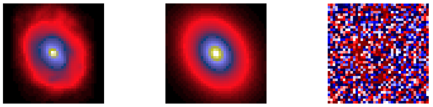
Analytic Sersic profile
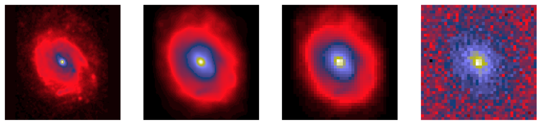
Modelling astro images
Galaxy light profile
Telescope convolution
Instrument acquisition (pixelation)
Instrumental noise
Analytic Sersic profile
Residuals
In practice
(R*P*\sum_i M_i)_{[x,y]}+N_{[x,y]}
Alternatives
- Pixelated models: Every pixel is a free parameter
- Machine learning model
- Basis decomposition:
- PCA
- Polynomials, shapelets
- Wavelets
- ...
M^{\star}(x, y) = \sum_i a_i F_i(x, y)
Pixelated model
I_{[x,y]} = R*P*M_{[x,y]} +N_{[x,y]}
I_{[x,y]}
Solution for M is not unique
Solution space:
M^{\star} \in M \setminus ||I-R*P*M||_2^2 < \epsilon
Pixelated model
I_{[x,y]} = P*M_{[x,y]} +N_{[x,y]}
I_{[x,y]}
Requires constraints
M^{\star} = \underset{M}{argmin}||I-R*P*M||_2^2 + C(M)
M^{\star} = \underset{M}{argmin}||I-R*P*M||_2^2 + ||M||_2^2
Example: limiting the 2-norm of the solution
Pixelated model
M^{\star} = \underset{M}{argmin}||I-R*P*M||_2^2 + C(M)
- Get creative about what constraints to use
- Example: The SDSS deblender: symmetry & Monotonicity
Robert Lupton

SCARLET
$$I_j = R*P_j * \sum_{i,n} a_{j,i,n}m_{i,n} +N_j$$
Melchior et al. 2016 ( arXiv:1802.10157)
- morphological assumptions as constraints:
- Positivity: All non-zero pixels must have positive values
- Monotonicity: Profiles smoothly decrease for the centre out.
-
Symmetry: Pixels about the central pixel take the value of the minimum of the two (Obsolete since Melchior, Joseph, Moolekamp 2019) - Bounding: Each galaxy profile is contained in a finite bounding box
SCARLET:
Modelling multi-band images
F435w
F606w
F814w
NASA/ESA: Hubble Frontier Fields, MACSJ 1149, Lotz et al. (2016)
- RGB images are collections of band in different filters
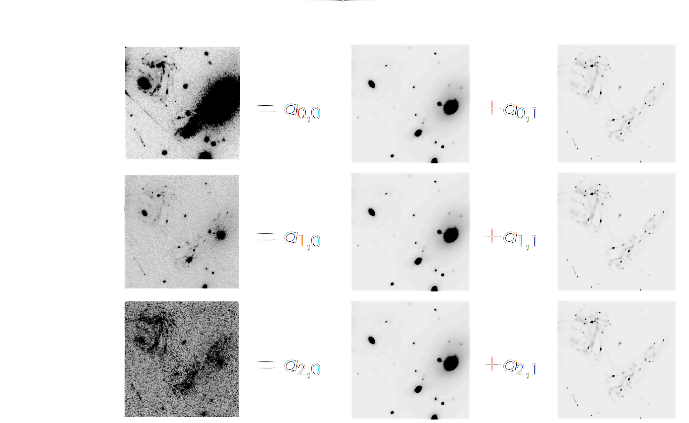
SCARLET
- Colour-based: each band is a linear combination of monochromatic components
F435w: \(I_2\)
F606w: \(I_1\)
F814w: \(I_0\)
$$I_j = R*P_j * \sum_i a_{j,i}m_i + N_j$$
$$m_0$$
$$m_1$$
$$I$$
SCARLET
Melchior et al. 2016 ( arXiv:1802.10157)
Linear Optimisation
Constraints: Positivity, Monotonicity, Bounding.
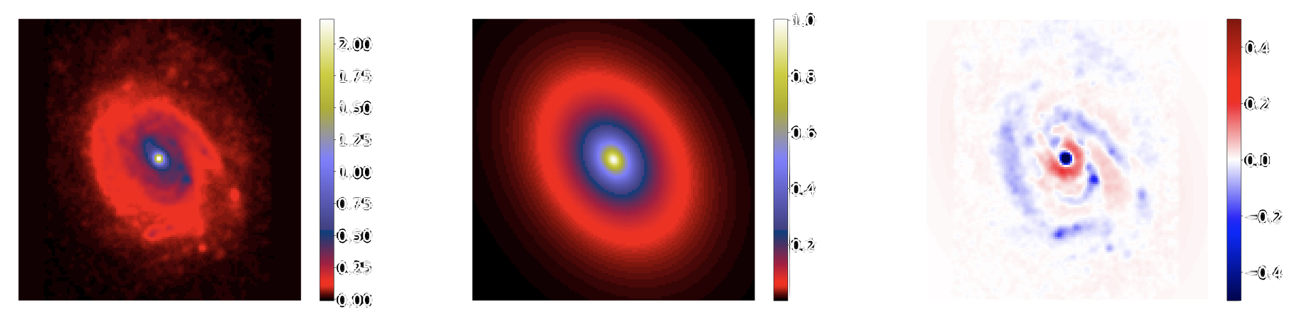
SCARLET
Melchior et al. 2016 ( arXiv:1802.10157)
Weakness (of the model): Monotonicity can causes trails and shadows.
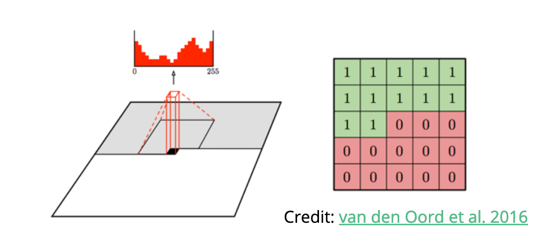
Functional decompositions:
The Starlet transfrom
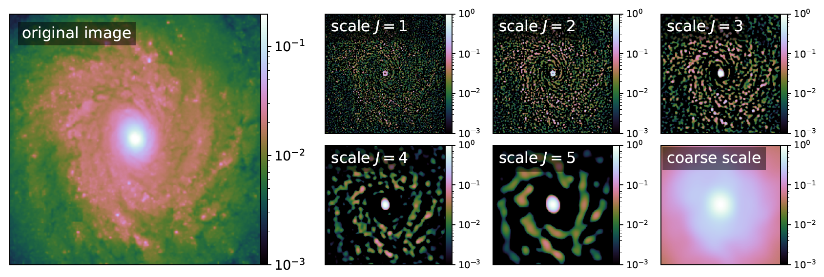
Starlet coefficients
- Multiscale transformation
- Decomposition in B-splines at different spatial scales
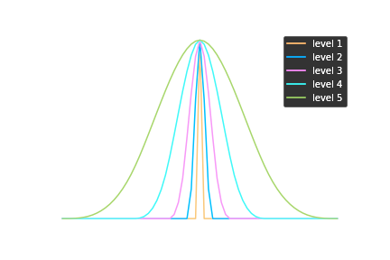
Starlet basis set
Functional decompositions:
The Starlet transfrom
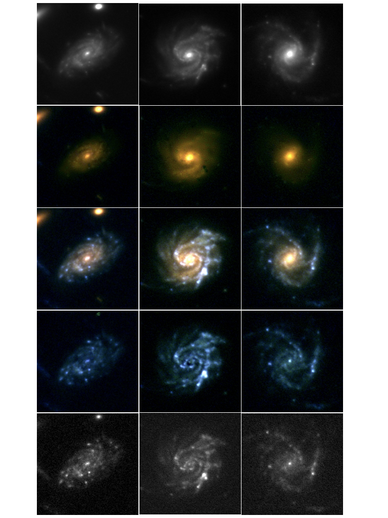
Illustration: Detection in crowded fields
Credit: Fred Moolekamp
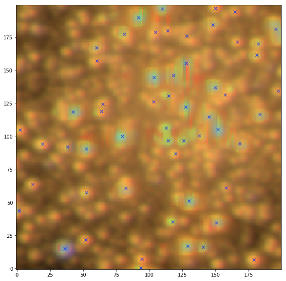
NGC 6569
Sep detection
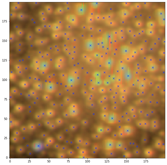
NGC 6569
Starlet+Sep detection
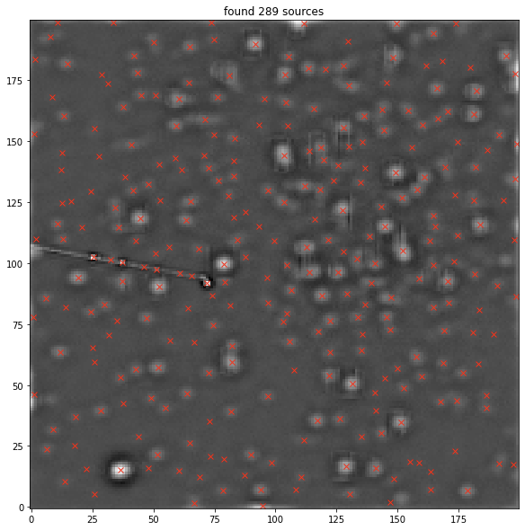
NGC 6569
Starlet level 1
Constraints on starlet coefficients
Is achieved by reconstructing sparse fields in starlets:
\( \tilde{S} = \underset{S}{argmin}\) \( \frac{1}{2}||I-HA\Phi S||^2_2 \) \(+\) \(\lambda||S||_1\) \(+\) \(\mathcal{i}_+(\Phi S) \)
Likelihood Sparsity Positivity
(smoothness constraint)
MuSCADeT: Joseph et al. 2016 (arxiv:1603.00473)
$$I_j = R*P_j * \sum_i a_{j,i}\Phi s_i + N_j, \qquad m_i = \Phi s_i$$
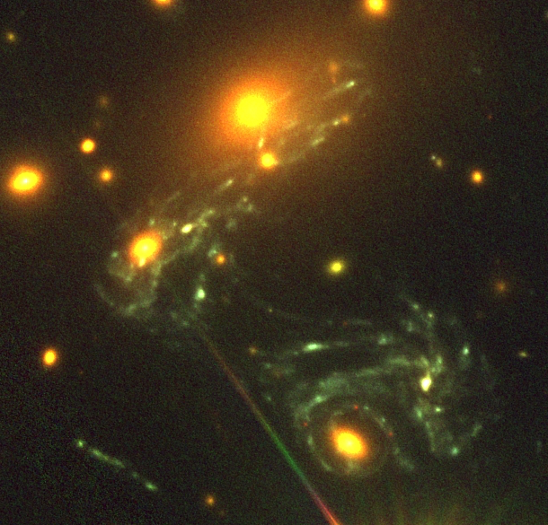
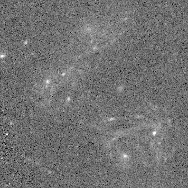
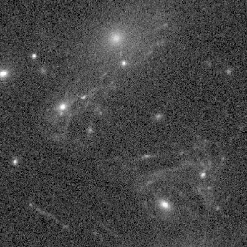
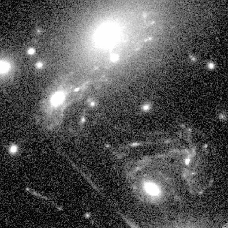
NASA/ESA: Hubble Frontier Fields, MACSJ 0416, Lotz et al. (2016)
Complex galaxies
F814w
F435w
RGB
MuSCADeT Red
MuSCADeT Blue
Low Surface Brightness Galaxies
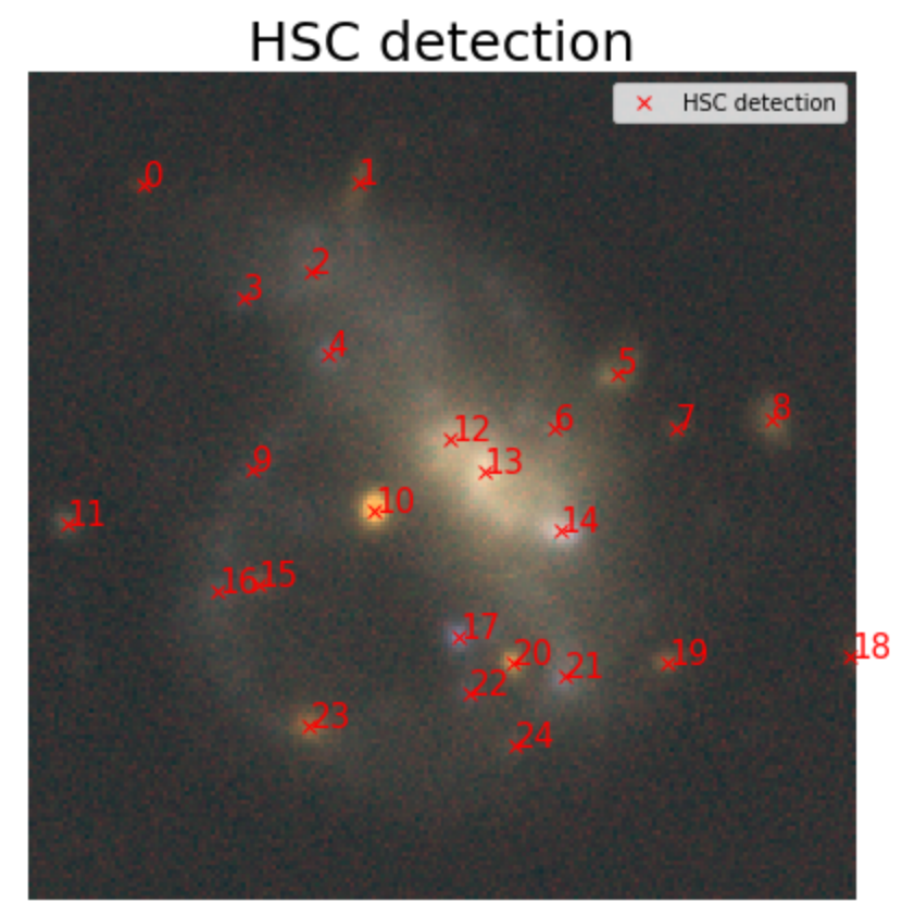
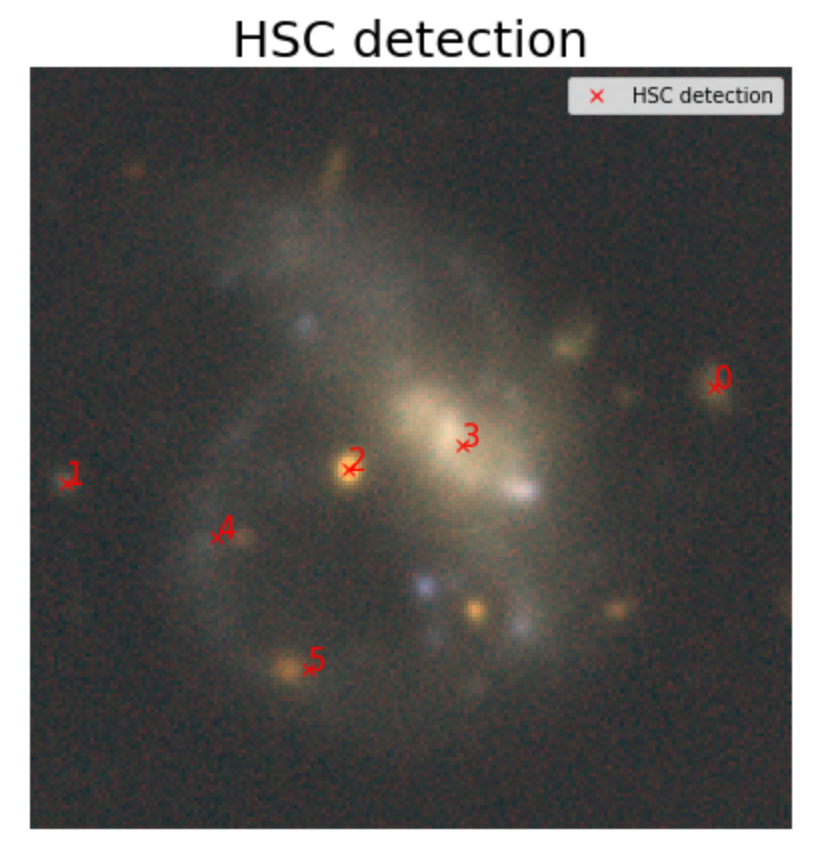
Sep detection
Starlet + Sep detection
On going work with Johnny Greco
Low Surface Brightness Galaxies
On going work with Johnny Greco
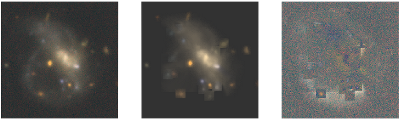
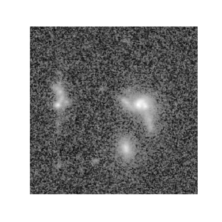
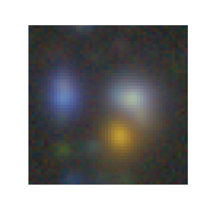
Data
Scarlet model
Residuals
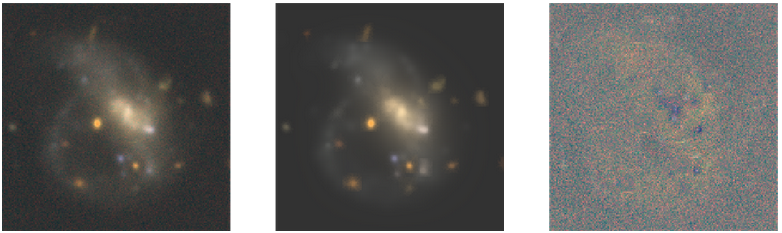
Monotonicity + Positivity:
Starlet sparsity + Positivity:
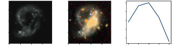
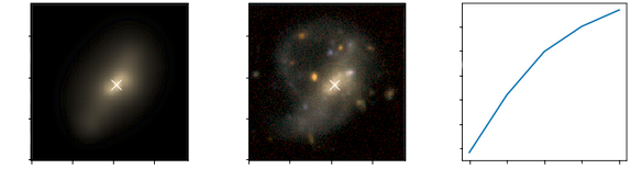
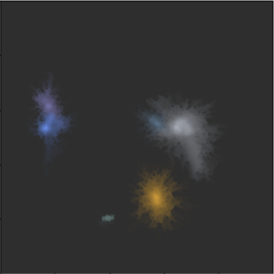
Low Surface Brightness Galaxies
On going work with Johnny Greco
Starlet sparsity + Positivity:
Model
Spectrum
g r i z y
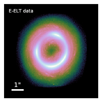
Reconstruction of strongly lensed source
I_{[x,y]} = F(R*P*M)_{[x,y]}+N_{[x,y]}
Reconstruction of strongly lensed source

Disclaimer: it can be improved
$$I_{j\in [0,k]} = H P_j * \sum_{i,n} a_{j,i,n}s_{i,n} + N_j$$
SCARLET
- Scarlet is flexible enough to handle models at a resolution different from the data. Now \(H\) accounts for the resampling of the model.
HST cosmos, F814w
HSC DR2, grizy
\(I_1\)
\(I_2\)
$$I_{j\in [k+1,n]} = R * P_j * \sum_{i,n} a_{j,i,n}s_{i,n} + N_j$$
pixels
wavelength
pixels
pixels
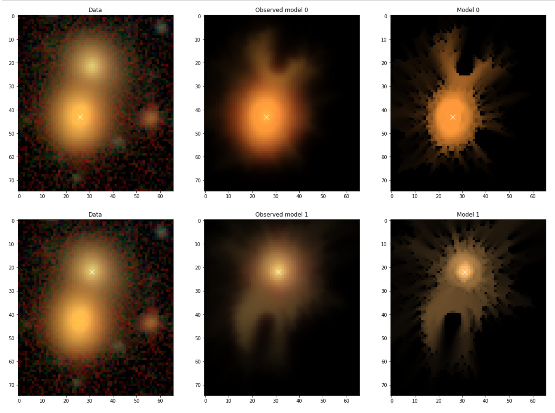
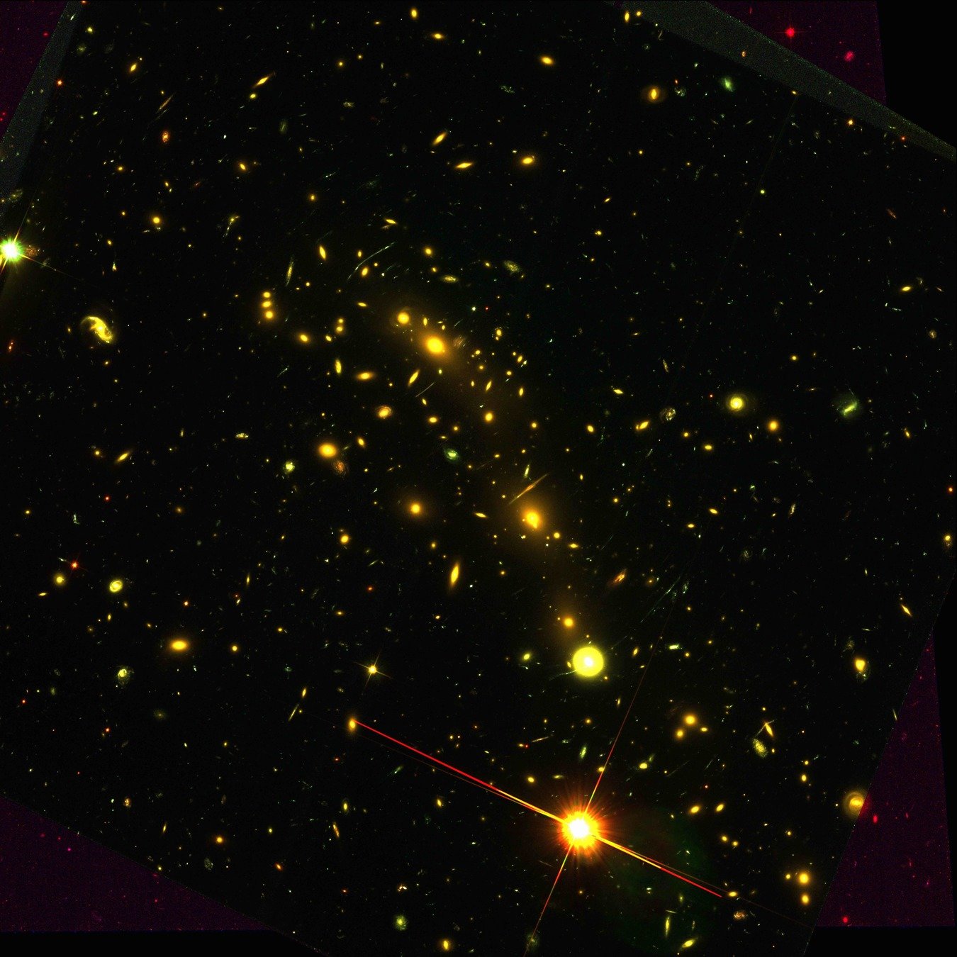
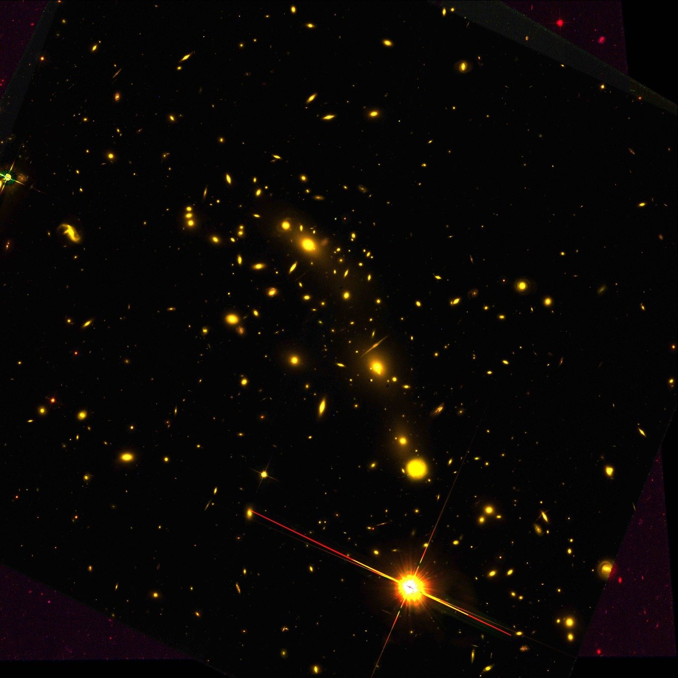
Combining surveys at different resolutions
HST cosmos, F814w
HSC DR2, grizy
\(I_1\):
\(I_2\):
pixels
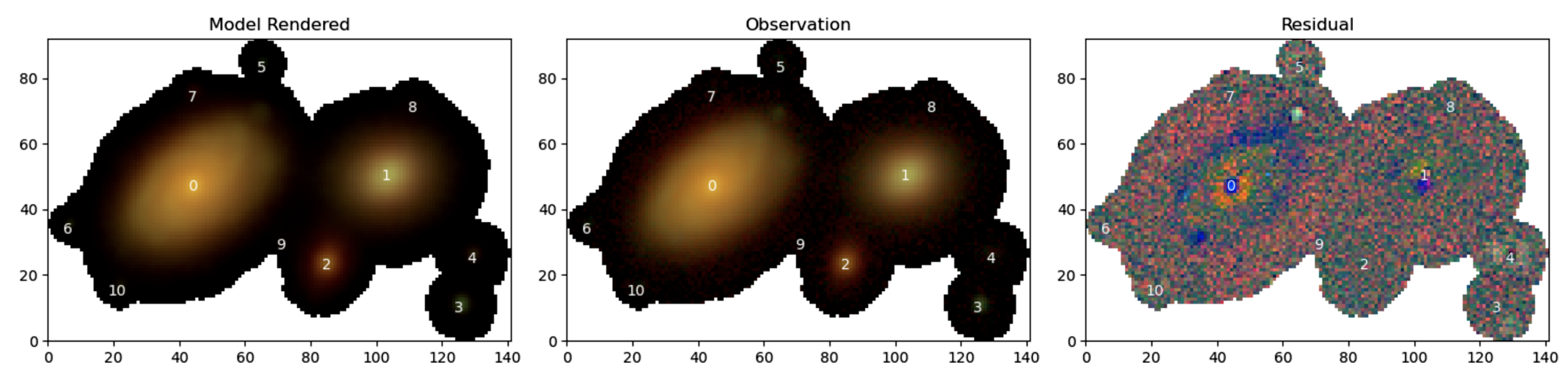
SCARLET
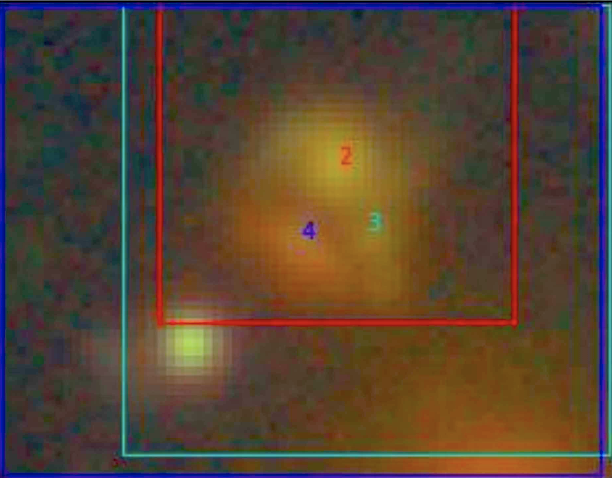
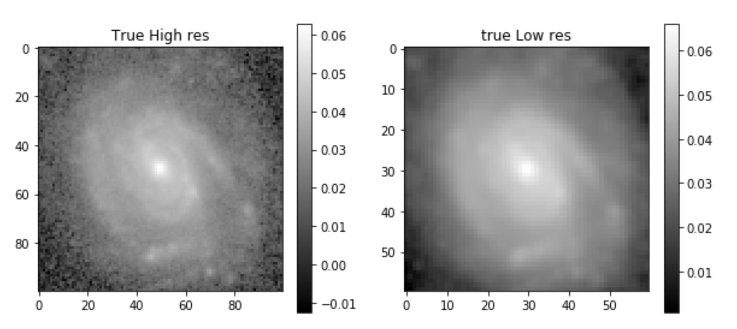
Multi-resolution fitting: Finding a model at high resolution that fits datasets at different resolutions:
\(I_1\)
\(I_2\)
\( \tilde{M} = \underset{M}{argmin}\) \( \frac{1}{2}||I_1-HPAM||^2_2 \) \(+\) \( \frac{1}{2}||I_2-RP'AM||^2_2 \)\(+\)\(\sum_i p(m_i)\)
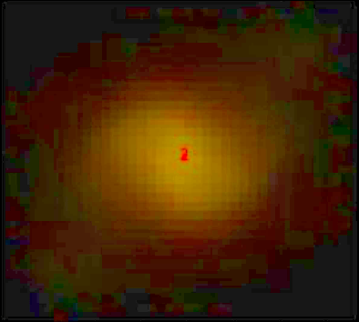
High resolution
Low resolution
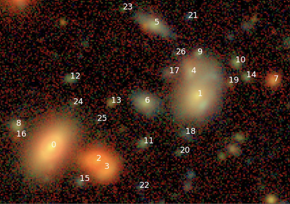
HST cosmos, F814w
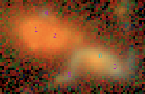
HSC DR2, grizy
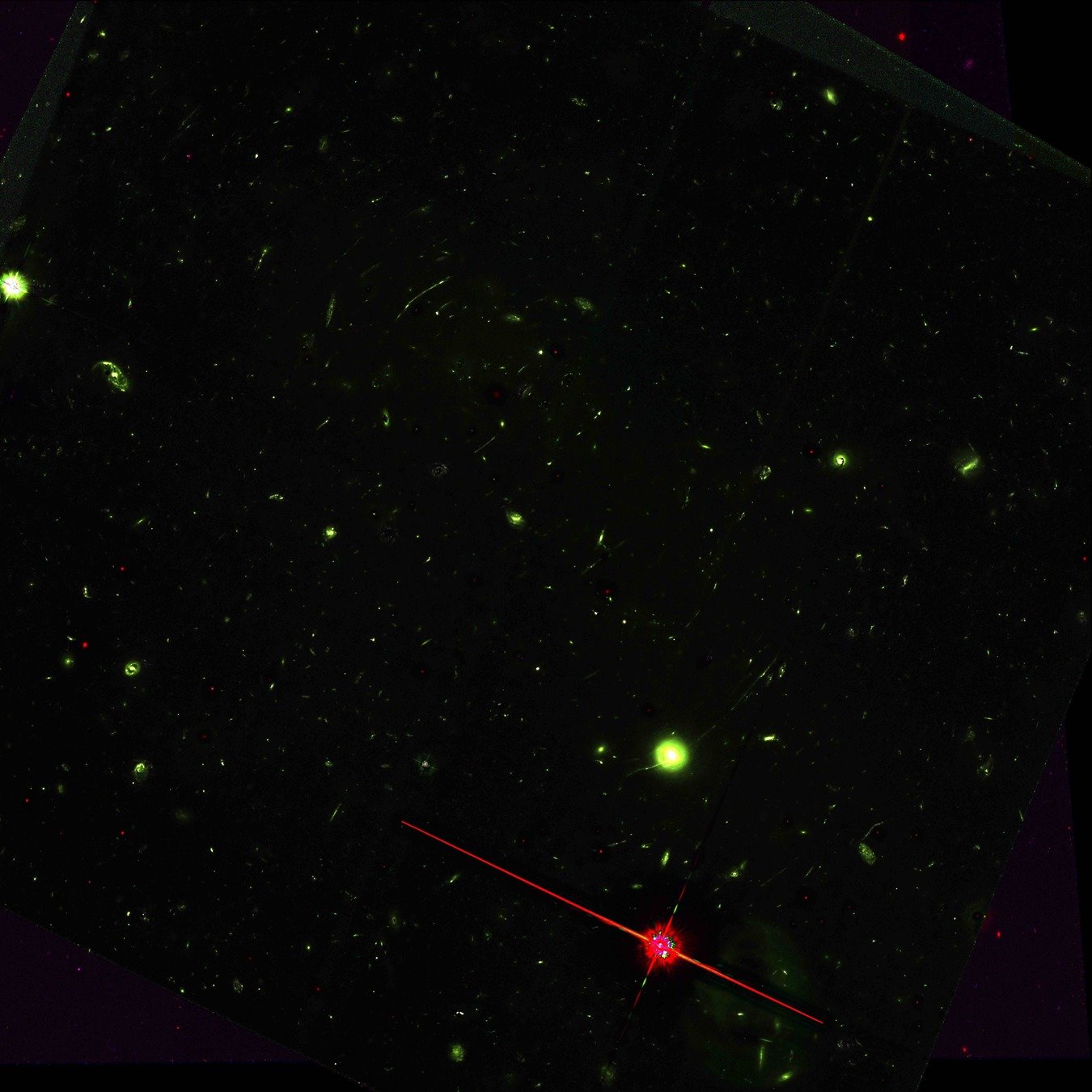
Scarlet model
1
2
4
3
5
6
1
2
4
3
5
6
1
2
4
3
5
6
$$I_j = R*P_j * \sum_{i,n} a_{j,i,n}m_{i,n}$$
SCARLET
- Scarlet is flexible to the kind of constraints we can impose on morphology. We are now implementing priors from machine learning Lanusse et al. 2019:
$$p(m) = \prod_k p(m_k|m_{k-1}, ..., s_0) $$
\( \tilde{M} = \underset{M}{argmin}\) \( \frac{1}{2}||I-RPAM||^2_2 \) \(+\) \(\sum_i p(m_i)\)
Last thoughts
-
Modelling images:
- Understanding the formation of images
- Incorporating assumptions as prior:
- Knowledge of galaxy morphology: Symmetry, Monotonicity, Smoothness (sparsity), Positivity
- How to incorporate dust?
- Data can get even more complicated:
- Integral Field Units
- spectral information
- varying PSF
- Reconstructing shear/lensing maps
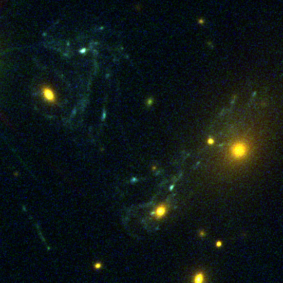
MuSCADeT
The algorithm
- Gradient step
- Find S close from U with the smallest \(\ell_0\) norm
- Set negative entries to 0
$$U \gets S+\mu A^T H^T (Y-HAS)$$
$$S \gets \Phi \underset{\alpha_S}{argmin}\frac{1}{2}||U-\Phi\alpha_S||_2^2+\lambda|| \alpha_S||_0$$
$$S[S<0]\gets 0$$
- Estimate the mixing matrix A
MuSCADeT
The algorithm
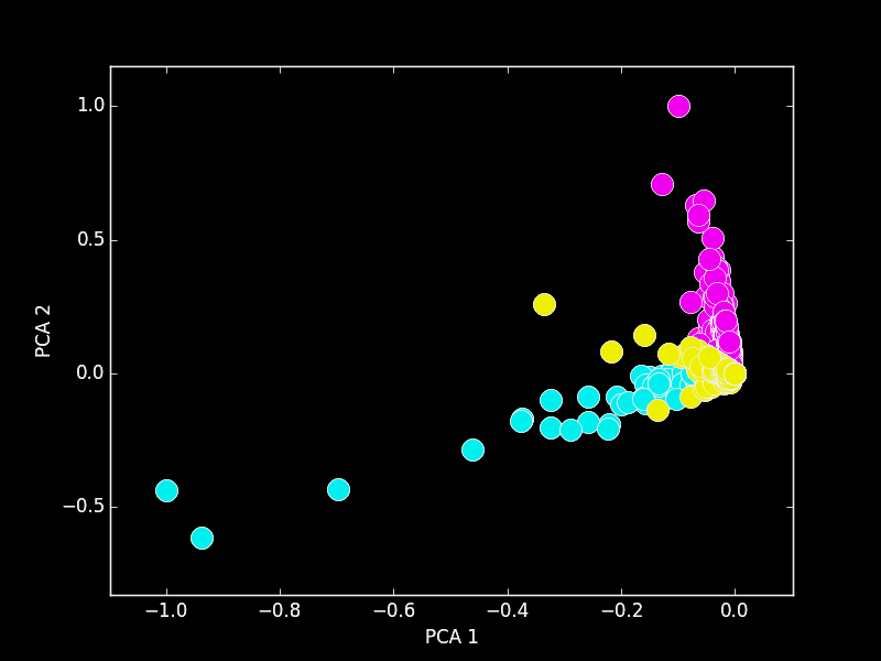
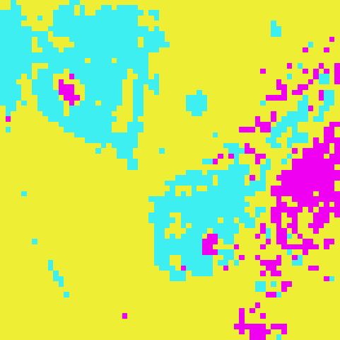
- Estimate the mixing matrix A (default)
Colours are extracted from the scene using Principal Component Analysis (PCA) of the multi-band pixels
The problem of speed
\(f_2(X, Y) = \sum_{x_k, y_j} f_1(x_k, y_j) P(X-x_k, Y-y_j)\)
As many operations as there are distances between red and blue points, i.e. \(M^2N^2\)
M
N
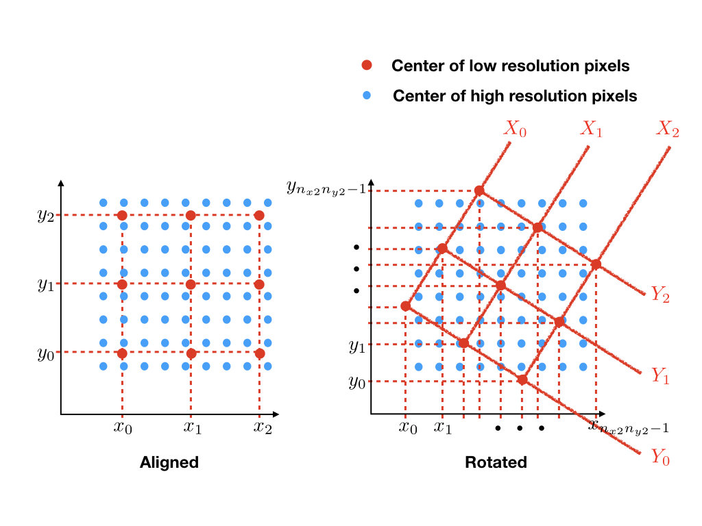
Interpolation at different resolution
Euclid-like
HST-like
Resampling and difference convolution can be done as one operation:
\(M(X, Y) = \sum_{x_k, y_j} m(x_k, y_j) H(X-x_k, Y-y_j)\)
Interpolation with difference kernel as the interpolation kernel. (Demo-ish in back up slide)
\(H(x,y) = \mathcal{F}^{-1}(\frac{\tilde{p_2}}{\tilde{p_1}})(-x,-y)\)
The problem of speed
\(f_2(X, Y) = \sum_{x_k, y_j} f_1(x_k, y_j) P(\frac{X}{h}-x_k, \frac{Y}{h}-y_j)\)
Reformulate to share the distance calculations along directions of constant coordinates:
\(f_2(X, Y) = \sum_{x_k, y_j} f_1(x_k-X_1cos\theta, y_j+X_1sin\theta) \times P(-Y_1sin\theta-x_k, -Y_1cos\theta-y_j)\)
\(X = hX_1cos\theta + hY_1sin\theta\)
\(Y = -hX_1sin\theta + hY_1cos\theta\)
Shifts along two directions
The problem of speed
\(f_2(X, Y) = \sum_{x_k, y_j} f_1(x_k-X_1cos\theta, y_j+X_1sin\theta) \times P(-Y_1sin\theta-x_k, -Y_1cos\theta-y_j)\)
- Shifts along \(2\times M\) directions instead of \(M^2\)
- Multiplcation of two matrices : \(N^2M \times MN^2 = M^2N^2\) operations
- Orders of magnitude faster than computing and multiplying by the \(P(X-x_k, Y-y_j)\) kernel
Interpolation kernel is actually a sinc
\(f_2(X) = (f_1*P)(X) = (\sum_{x_k} f_1(x_k)sinc(\frac{X-x_k}{h}))*(\sum_{x_p}P(x_p)sinc(\frac{X-x_p}{h}))\)
\(f_2(X) = (f_1*P)(X) = \sum_{x_k} f_1(x_k)\sum_{x_l}P(x_l)sinc(\frac{X-x_k - x_l}{h})\)
\(f_2(X) = (f_1*P)(X) = \sum_{x_k} f_1(x_k)\sum_{x_l}P(x_l- X)sinc(\frac{x_k + x_l}{h})\)
Making sure we get the pixel response right
\(I_2(x_{i2},y_{j2}).\) = \((rect_{h_1}*(f*p_1) *{F}^{-1}(\frac{\hat{rect_{h_2}}}{\hat{rect_{h_1}}}\frac{\hat{p_2}}{\hat{p_1}}))(x_{i2},y_{j2})\)
\(I_2(x_{i2},y_{j2}) = (rect_{h_2}*p_2*f)(x_{i2},y_{j2})\)
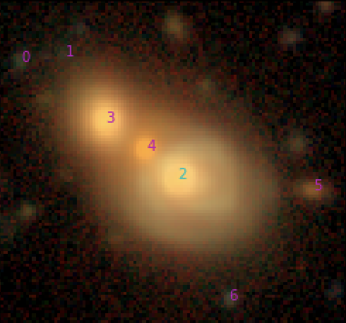
Deblending
By herjy


