Scalable Bayesian inference with automatically differentiable simulators for the cosmological analysis of the DESI survey


2026/09/25
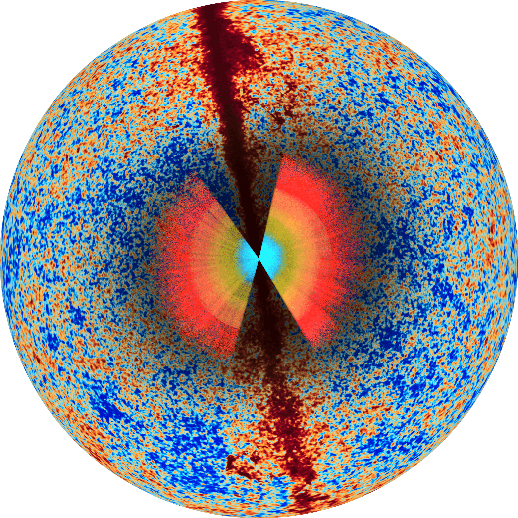
Mapping the Universe
- In the 1920s, we discovered the Universe is not limited to our galaxy and is expanding
- Galaxy further away
= light more shifted to the red
= Universe expanded more since emission
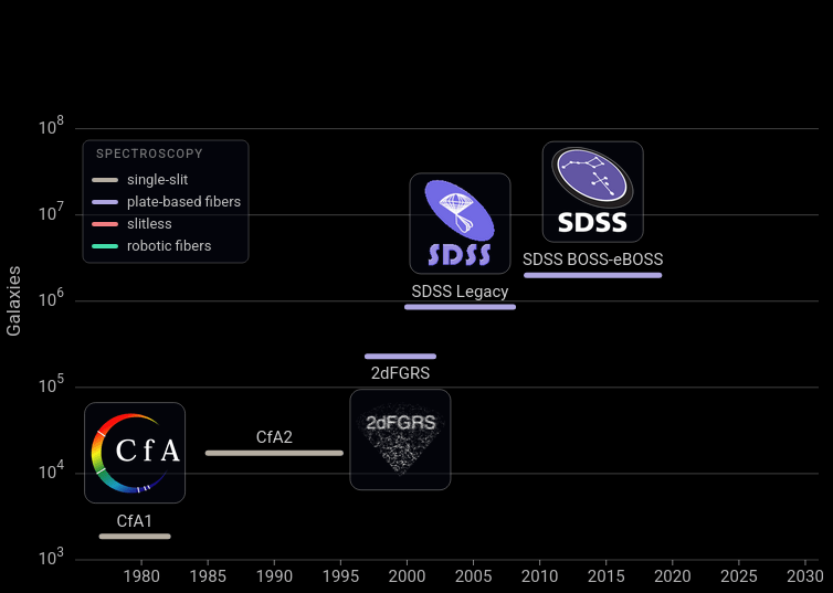
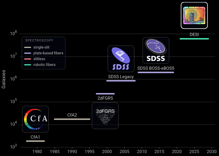
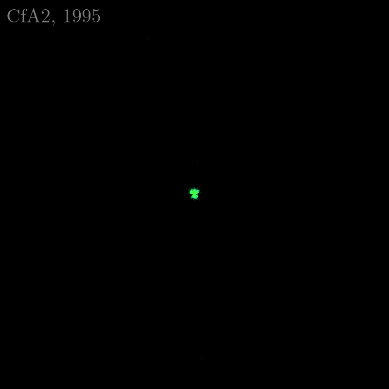
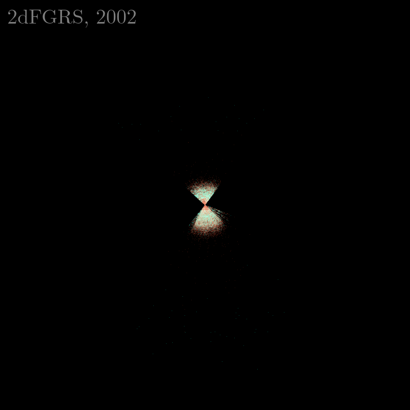
- In the 1970s, redshift surveys started mapping the Universe
- galaxies mapped \(\times 10\) every 10 years, thanks to spectroscopic improvements
DESI: \(60\)M by 2029
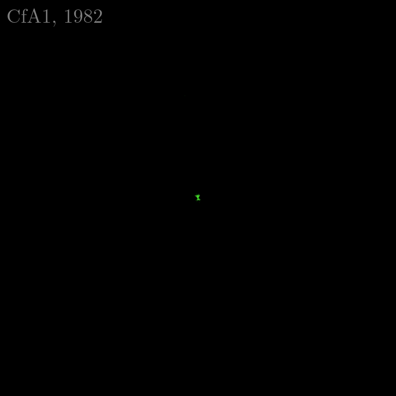
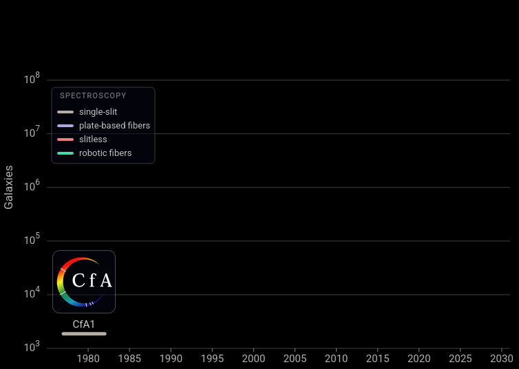
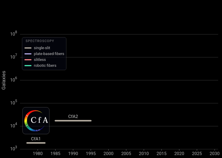
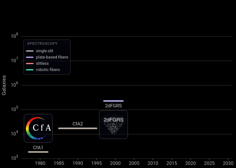
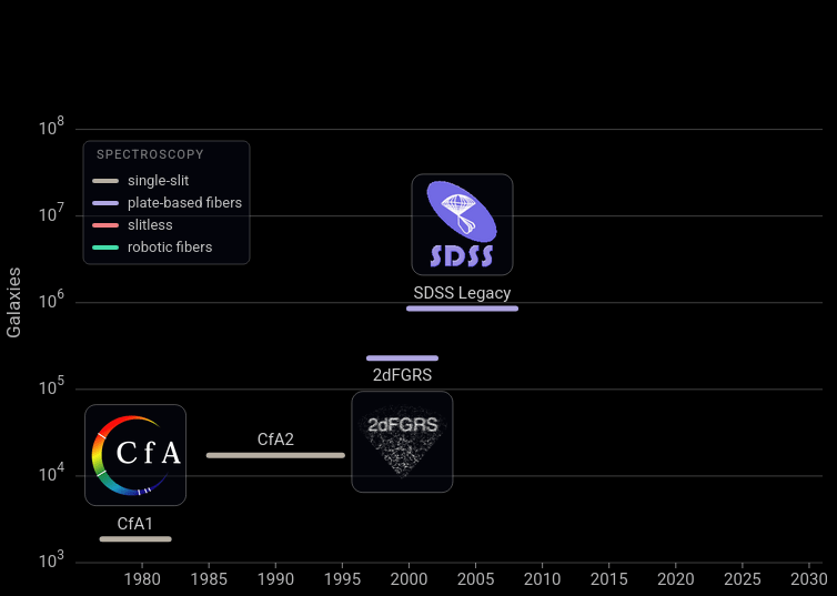
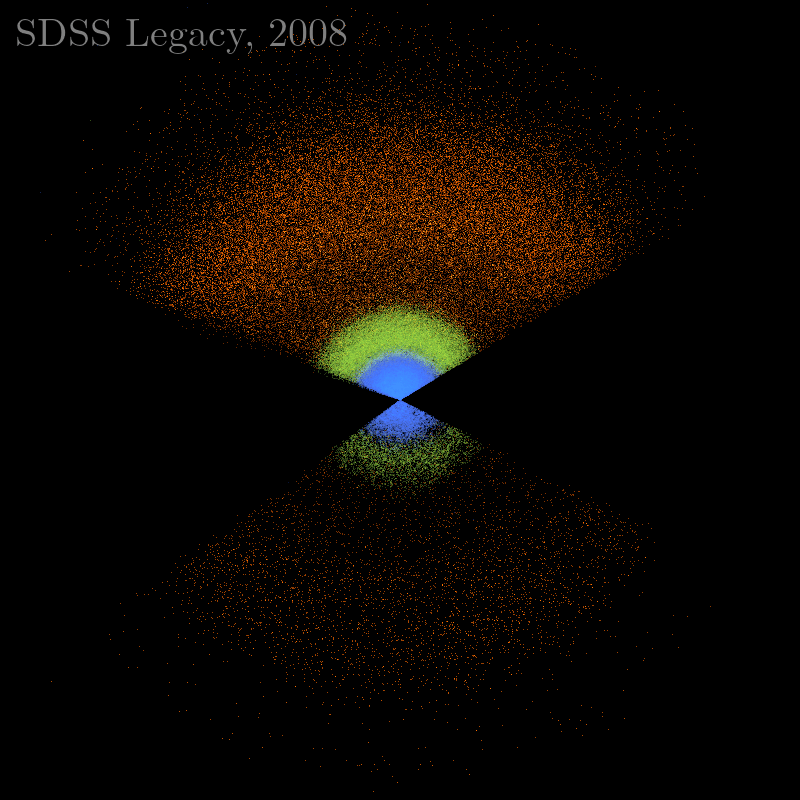
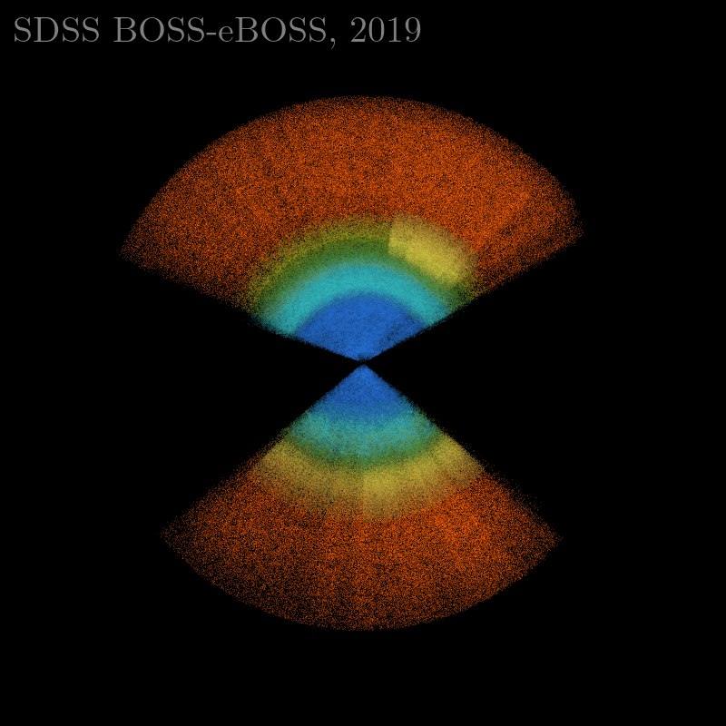
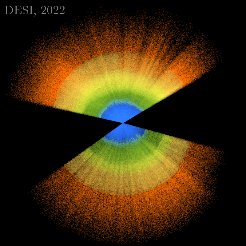
you are here
The Dark Energy Spectroscopic Instrument
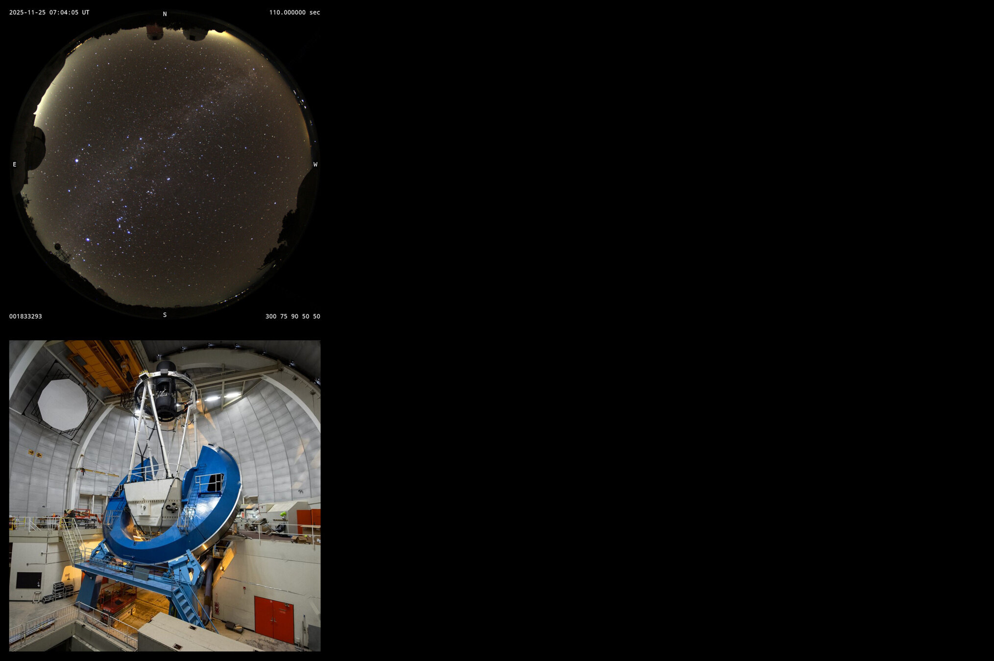

Observing shift 2025-11-25
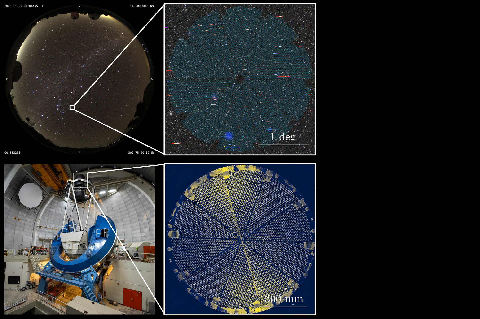
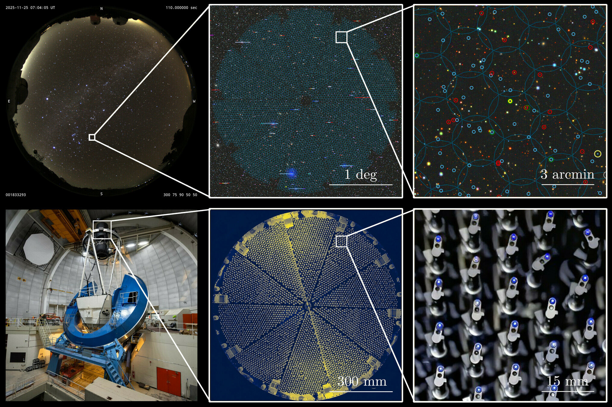
How did this happen?
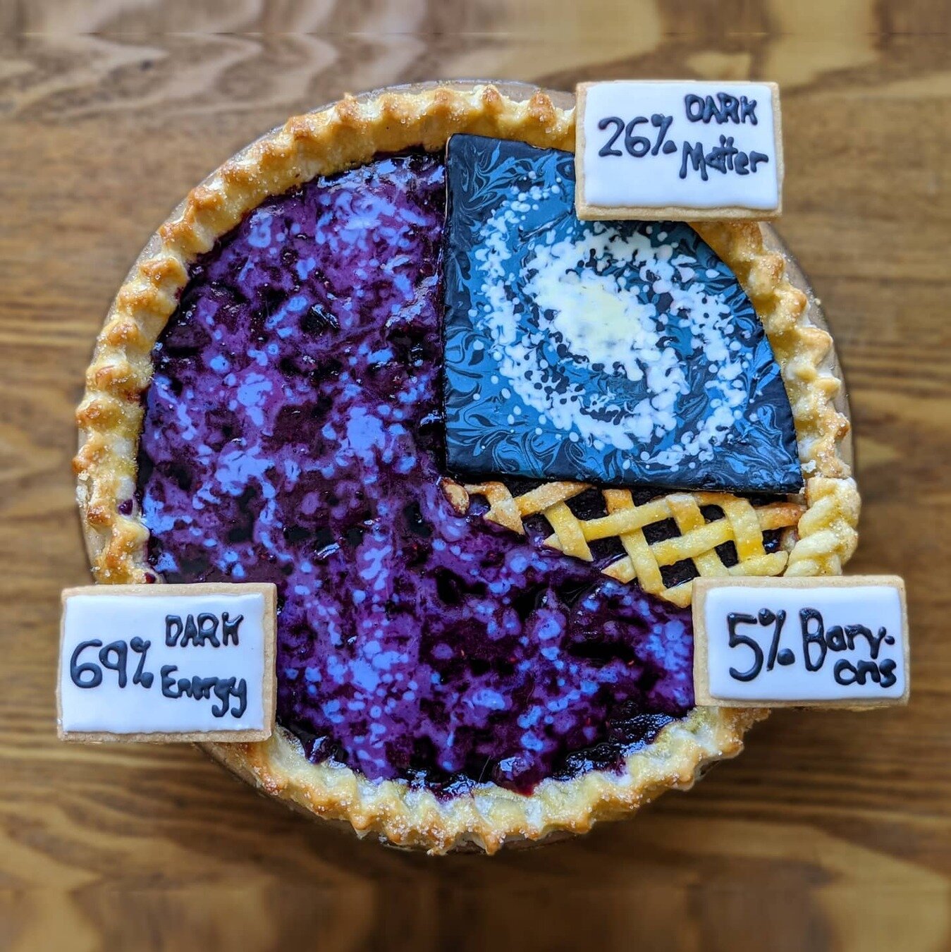
Which recipe for the Universe?
"A female kitchen chef amazed while discovering a cake made out of the universe with its large scale structures of galaxies."
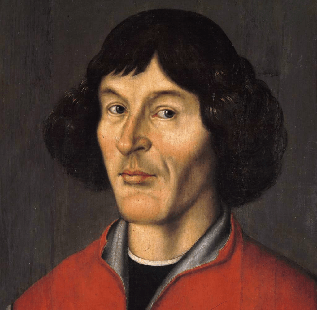
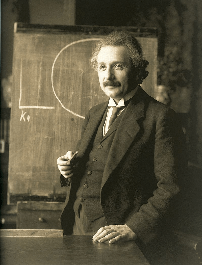
Copernicus, XVI CE
Einstein, XX CE
We are no privileged observers

$$G_{\mu\nu}= \kappa T_{\mu\nu}$$
Consequence:
Evolution of the Universe is determined by its content
A starter to a recipe...
Consequence:
Universe looks the same everywhere and in every direction
...remains to find the ingredients...
+

light
ordinary matter


dark matter
dark energy


❌
?
...but in what proportions?
...but in what proportions?
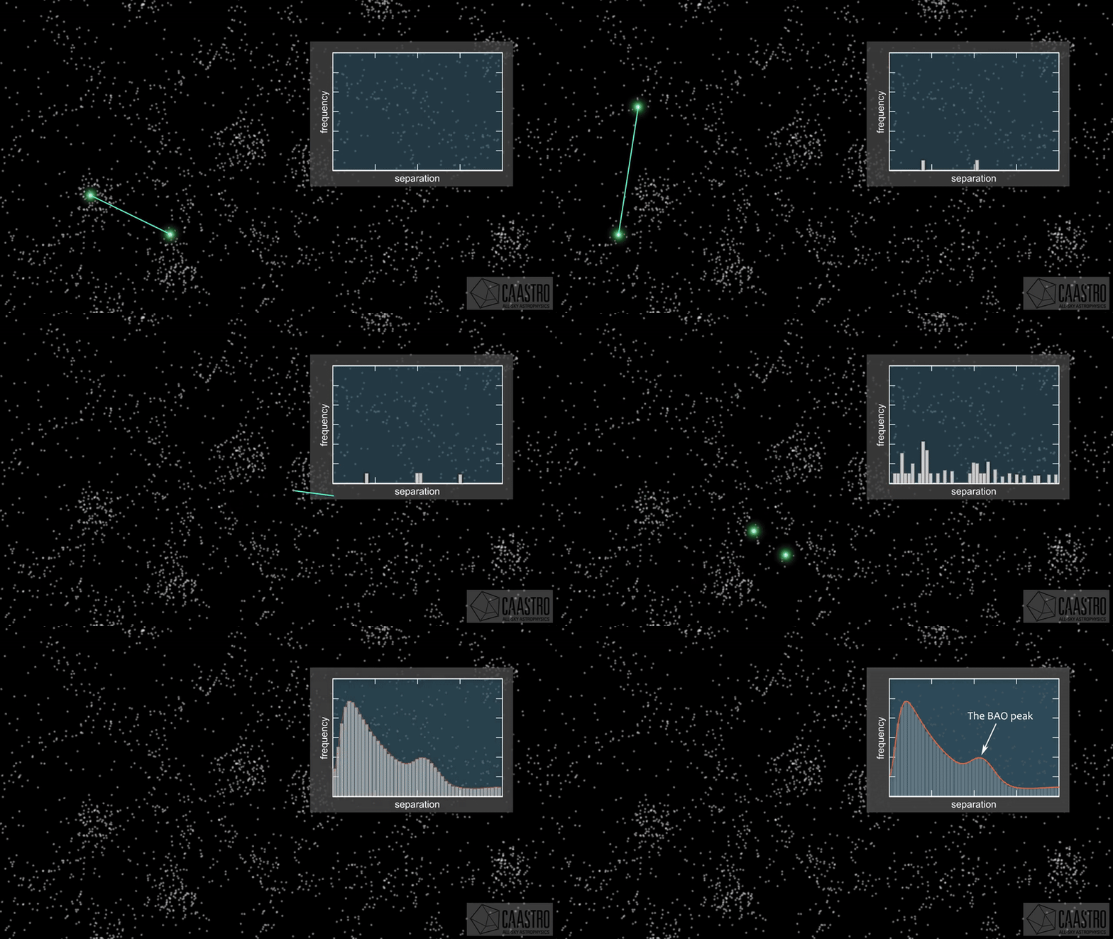
Standard analysis: compress the map
- At large scales, maps are Gaussian so 2PCF/power spectrum are lossless compression
- At small scales however, matter field is non-Gaussian
Gaussianity and beyond
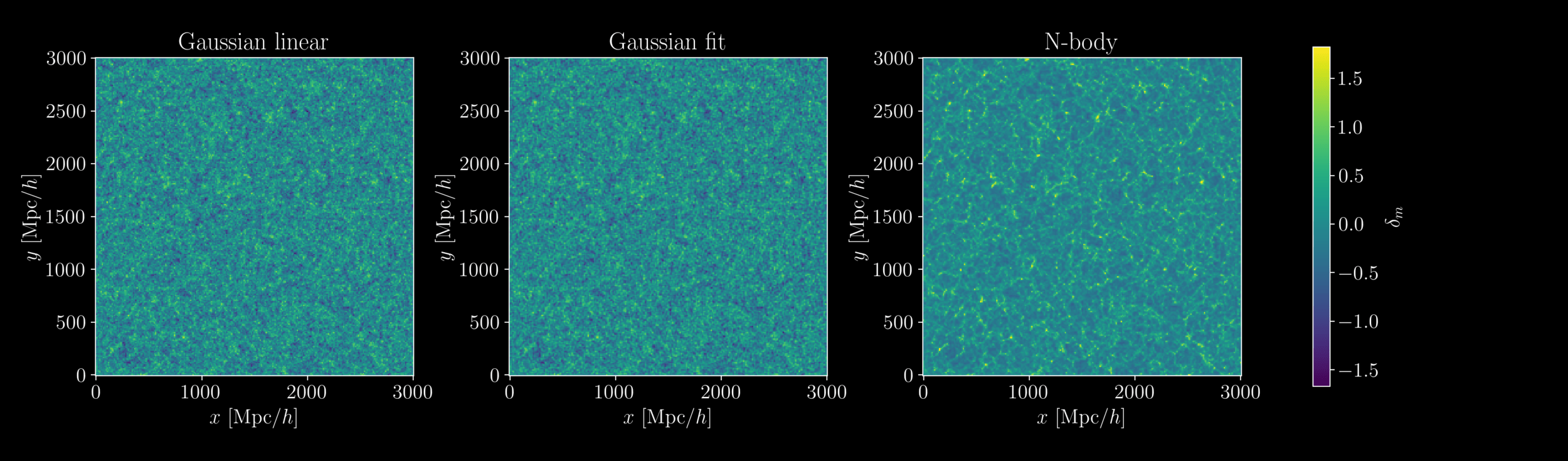
Gaussian
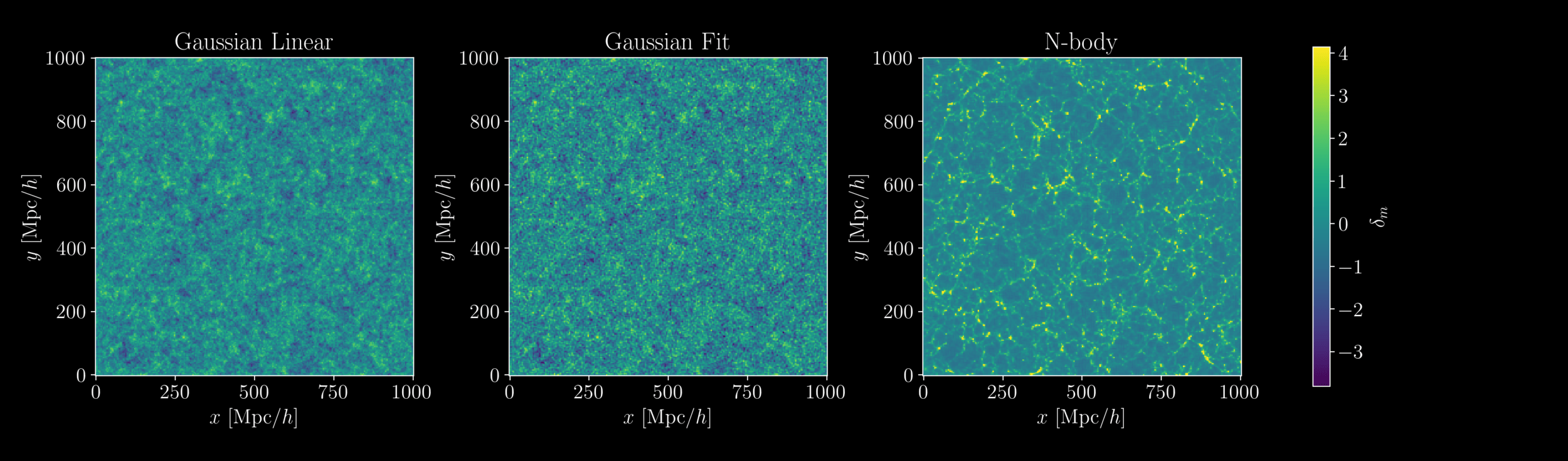
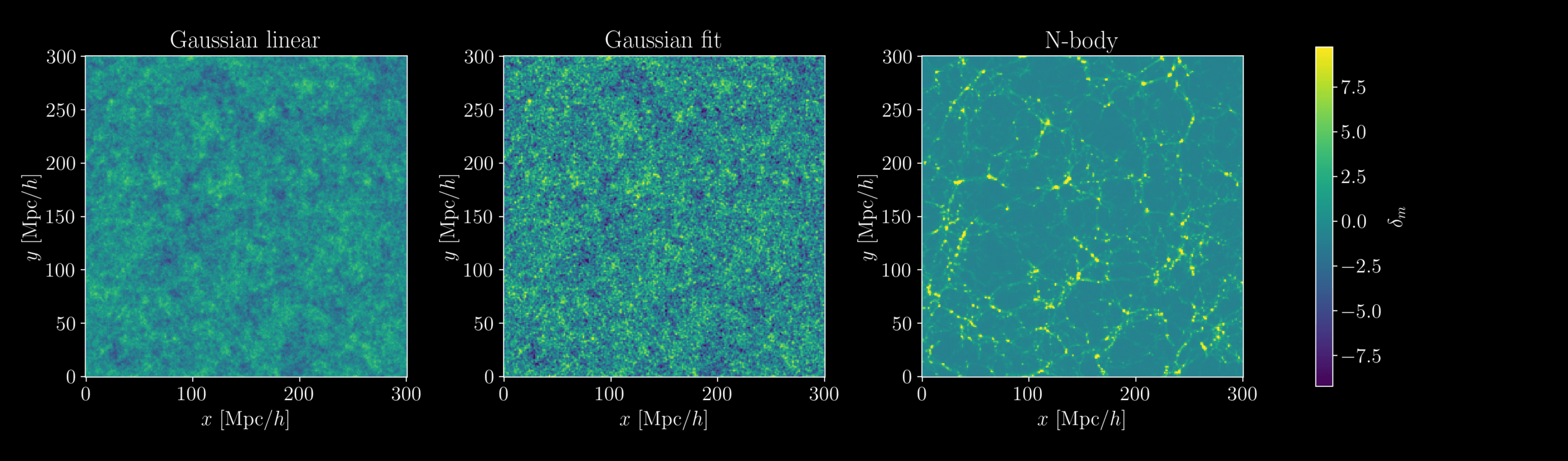
N-body (simulated gravity)
Same power spectrum
We gotta pump this information up
- Field-level
- CNN, GNN...
- WST, 1D-PDFs, Holes...
- Peak, Void, Split, Cluster...
- 3PCF, Bispectrum
- 2PCF, Power spectrum
- Power spectrum provides only Gaussian, 2-point, information
- To prospect smaller non-Gaussian scales, let's add:
- all the data
- learn the stat
- multiscale count
- object correlations
- more correlations
- standard analysis
Information content
Field-Level Inference
\(\delta_L\)
\(\Omega\)
\(\delta_g\)
\(\Omega := \{ \Omega_m, \Omega_\Lambda, H_0, \sigma_8, f_\mathrm{NL},...\}\)
\(\delta_L\)
\(\Omega\)
\(\delta_g\)
\(\delta_g\)
simulate & compare
update
observed
simulated
The Challenges:
- requires accurate modeling of the fields (likelihood)
- requires high-dimensional sampling:
to probe DESI volume at \(15\ \mathrm{Mpc}/h\), \(\operatorname{dim}(\delta_L) \simeq 1024^3\)
The Promise:
- lossless\(^*\) and explicit inference
Field-Level Inference


Simulating fields
- NumPyro
- Probabilistic Programming Language
(likelihood automatically derived from simulator) - Powered by JAX
- Probabilistic Programming Language
- JAX
- GPU acceleration
- Just-In-Time (JIT) compilation acceleration
- Automatic vectorization/parallelization
- Automatic differentiation

1. Gravity
Evolves linear matter field (initial conditions) \(\delta_L\) to non-linear matter field \(\delta_m\)
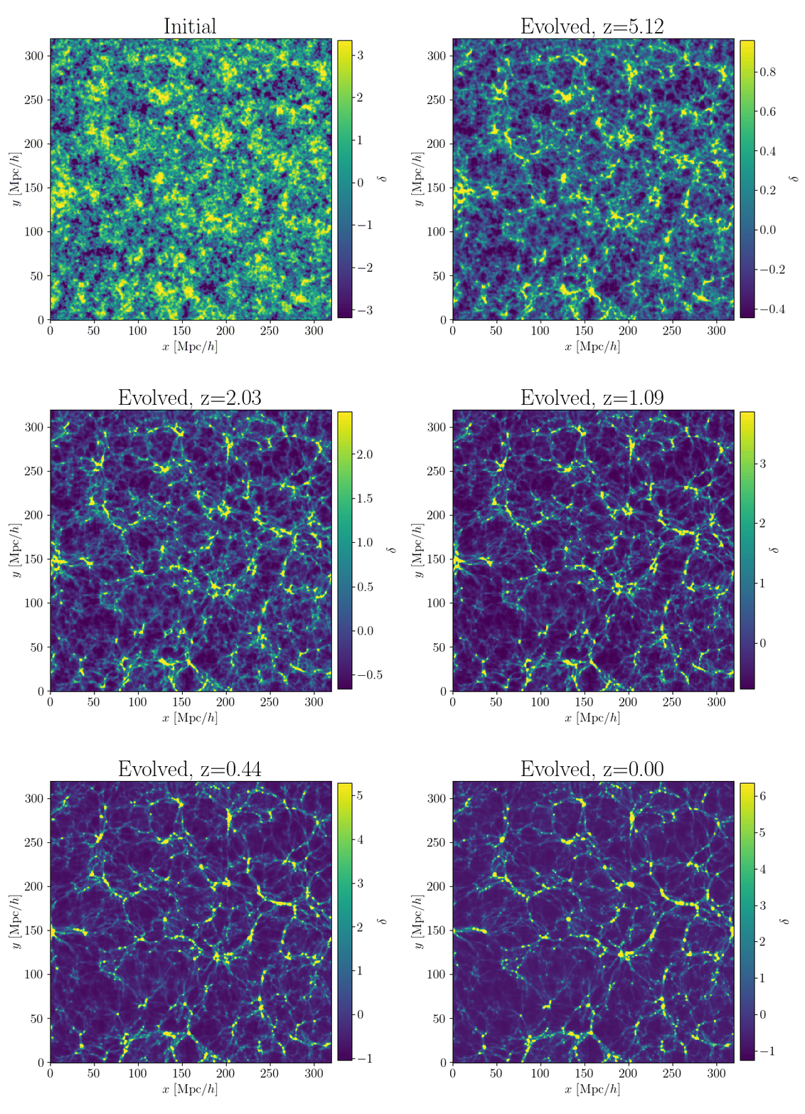
- Lagrangian Perturbation Theory
- 1LPT, 2LPT, ...
- Particle-Mesh (PM) N-body
- JaxPM, BullFrog
(Modi+2020, Rampf+2024)
- JaxPM, BullFrog
How to N-body-differentiate?
paint*
fft*
ifft*
read*

\(\delta(\boldsymbol x)\)
\(\delta(\boldsymbol k)\)

\((\boldsymbol q, \boldsymbol p)\)
apply forces
to move particles
\(\begin{cases}\dot {\boldsymbol q} \propto \boldsymbol p\\ \dot{\boldsymbol p} = \boldsymbol f \end{cases}\)
solve Vlasov-Poisson
to compute forces
\(\begin{cases}\nabla^2 \phi \propto \delta\\ \boldsymbol f = -\nabla \phi \end{cases} \implies \boldsymbol f \propto \frac{i\boldsymbol k}{k^2} \delta\)
*: differentiable, e.g. with , and in \(\mathcal O(n \log n)\)
2. Matter-galaxy connection
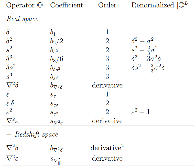
- \(\delta_g = b_1^E \delta_m\) similar to weight matter particles by
$$w_g = 1+{\color{purple} b_1} \delta_L$$ - Systematic approach as Effective Field Theory (EFT), expand in all operators that satisfy symmetries$$w_g = 1+\sum_{\mathbb O} {\color{purple} b^L_{\mathbb O}} [\mathbb O_{L}]$$
- Paint weighted particles on grid with kernel \(K\)
$$(1+\delta_g)(\boldsymbol x) = \int K(\boldsymbol x - \boldsymbol q^\mathrm{fin}) \mathcal w_g(\boldsymbol q^\mathrm{in})\, \mathrm d \boldsymbol q^\mathrm{in}$$
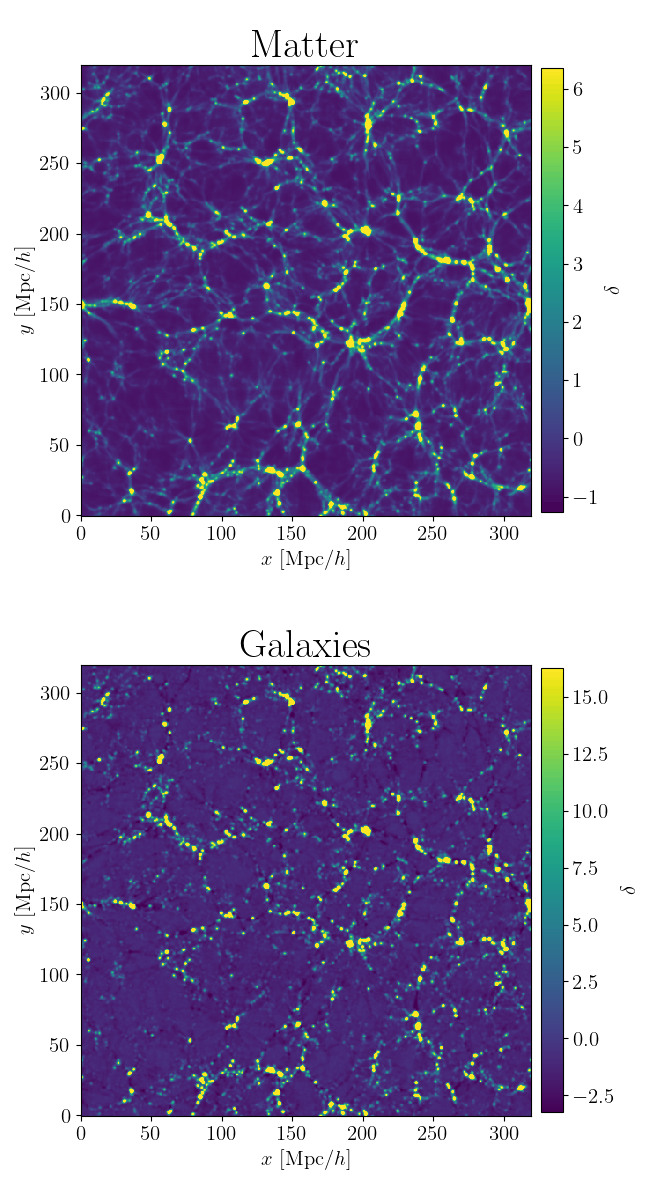
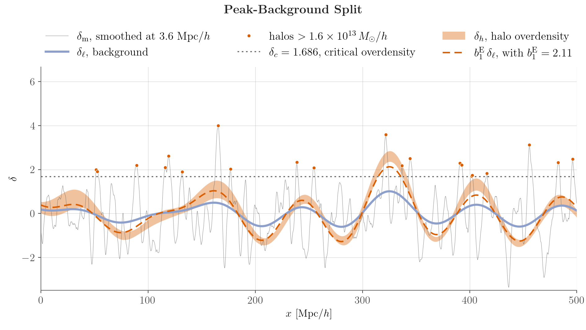
Halo hosts form where \(\delta_m > \delta_c \implies{\color{brown} \delta_g} \propto {\color{blue} \delta_m}\)
3. Redshift-space distortions and light-cone
2LPT solved using the fixed point method
$$z = \chi^{-1}(|\boldsymbol q + \Psi(\boldsymbol q, z)|)$$
(no interpolation needed)
Particles moved according to their peculiar velocities
$$\Delta\boldsymbol q= H^{-1}\dot {\boldsymbol q_\parallel}$$
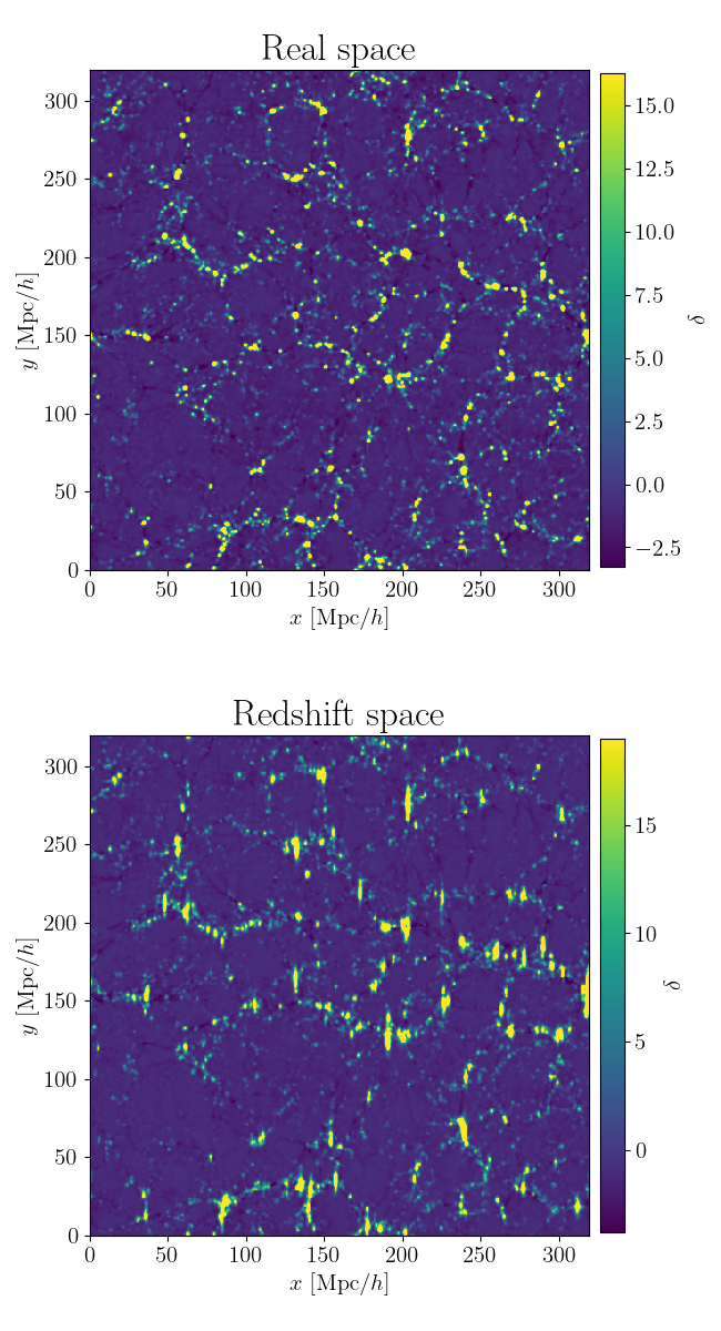
Galaxy peculiar velocities add up to cosmological redshift
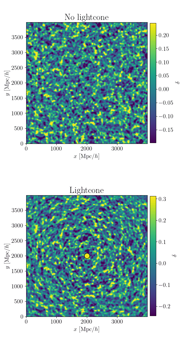
Far away galaxies are seen in younger, less evolved structures
\(k_\mathrm{evolve}, k_\mathrm{paint}\)
(gravity, EFT)
\(k_\mathrm{final}\)
\(k_\mathrm{init}\)
Fields in silico
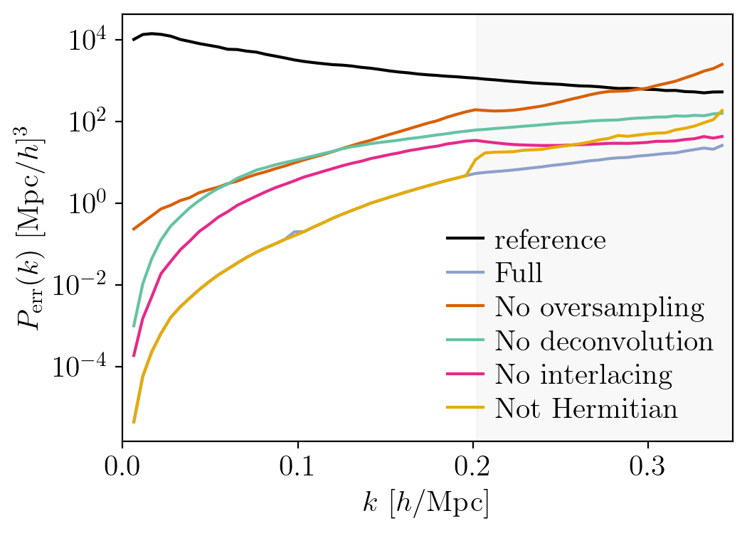
- Numerical fields are finite and discrete, manipulations can introduce unphysical artifacts (aliasing, smoothing...)
- Discreteness-mitigation methods, validated against DESI reference simulations N-body+HOD AbacusSummit
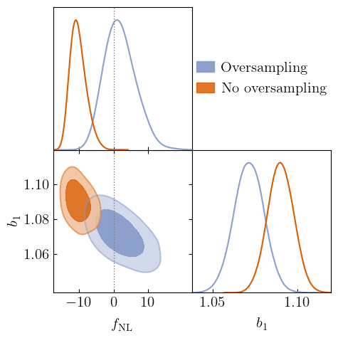
- Example: oversampling
- Otherwise, biased cosmological inference
\(P_\mathrm{err} = 0\)
\(\iff\)
equal fields
Sampling fields
- Our goal: sample a target distribution,
the posterior \(\Omega, \delta_L \mid \delta_g\)
- Classical MCMC algorithm:
- make agnostic move (Brownian motion)
- accept or reject samples based on their probability (Metropolis adjustment)
- Posterior statistics are estimated within Monte Carlo error \(\simeq n^{-1/2}\)
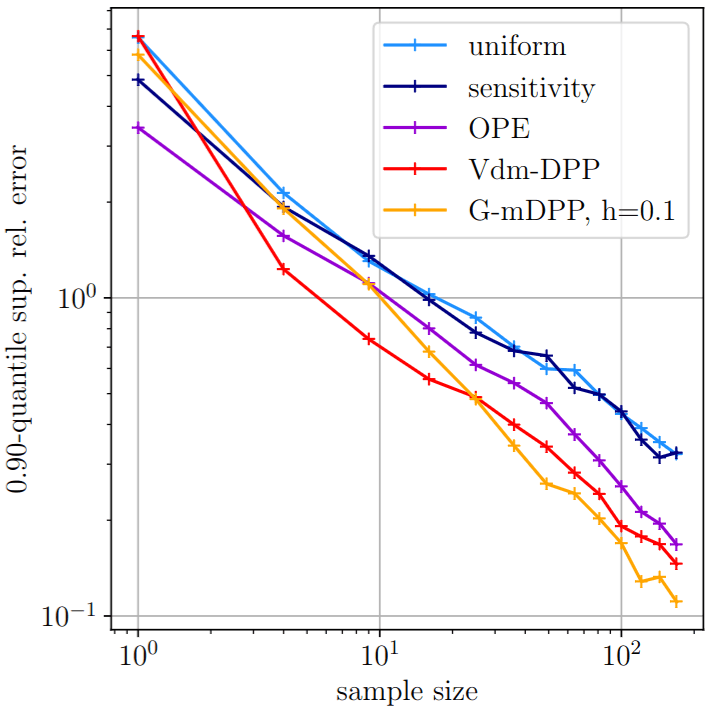
- In low dimension, can beat the \(n^{-1/2}\) rate by spreading samples more evenly...
(Bardenet, Ghosh, Simon, and Tran
NeurIPS2024 spotlight, alphabetical)
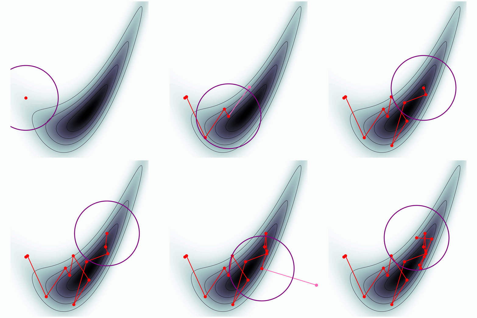
Metropolis-Hastings
High-dimensional sampling is hard
\(-\nabla\)
\(d \approx 1\)
🏠
🚶♀️
- To maintain constant acceptance probability: step-size \(\varepsilon\simeq d^{-1/2}\)
- Make no agnostic move but rather informed by gradient
- Brownian motion moves slowly: steps per traveled distance \(\simeq \varepsilon^{-2} \)
- Introduce momentum
- Introduce momentum
\(d \gg 1\)
🪺
🐦
Target to explore
Canonical MCMC samplers
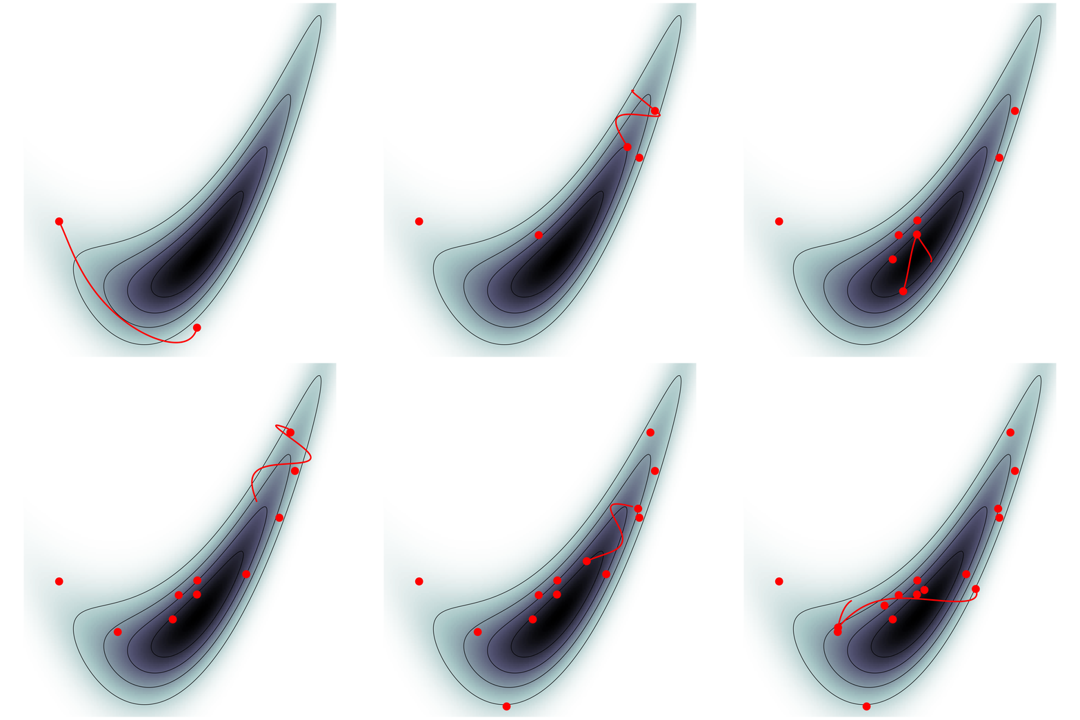
To sample from \(\mathrm p \propto e^{-U}\)
- take particle with position \(\boldsymbol q\), momentum \(\boldsymbol p\), and Hamiltonian $$\mathcal H(\boldsymbol q, \boldsymbol p) = U(\boldsymbol q) + \frac 1 2 p^2$$
- follow Hamiltonian dynamics during time \(L\)
$$\begin{cases} \dot {{\boldsymbol q}} = \partial_{\boldsymbol p}\mathcal H = {{\boldsymbol p}}\\ \dot {{\boldsymbol p}} = -\partial_{\boldsymbol q}\mathcal H = -{\color{red} \nabla U(\boldsymbol q)} \end{cases}$$and refresh momentum \(\boldsymbol p \sim \mathcal N(\boldsymbol 0, I)\)
- usually, perform Metropolis adjustment
- this samples canonical ensemble $$\mathrm p_\text{C}(\boldsymbol q, \boldsymbol p) \propto e^{-\mathcal H(\boldsymbol q, \boldsymbol p)} \propto \mathrm p(\boldsymbol q)\,\mathcal N(\boldsymbol 0, I)$$
scales poorly with dimension
must average over all energy levels
MicroCanonical MCMC samplers
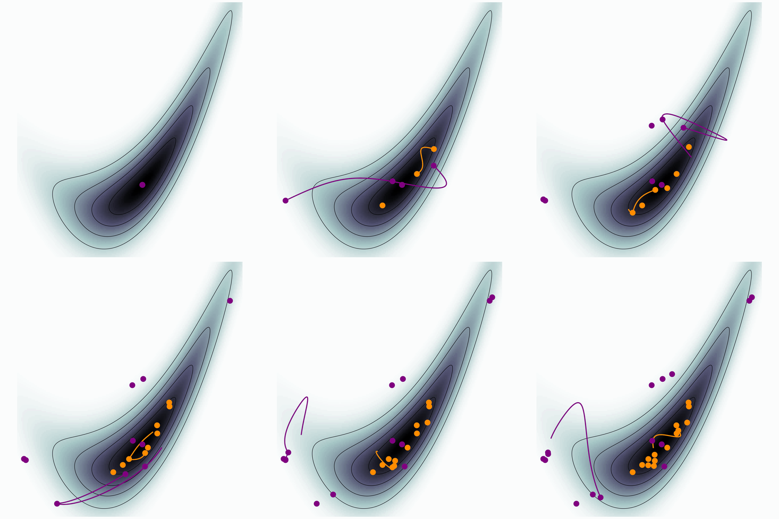
single energy/speed level
$$\mathcal H(\boldsymbol q, \boldsymbol p) = \frac {p^2} {2 m(\boldsymbol q)} - \frac{m(\boldsymbol q)}{2} \quad ; \quad m=e^{-U/(d-1)}$$
$$\begin{cases} \dot{\boldsymbol q} = \boldsymbol u\\ \dot{\boldsymbol u} = -(I - \boldsymbol u \boldsymbol u^\top) {\color{red}\nabla U(\boldsymbol q) }/ (d-1) \end{cases}$$ and refresh direction \(\boldsymbol u \leftarrow \boldsymbol z/ \lvert \boldsymbol z \rvert \quad ; \quad \boldsymbol z \sim \mathcal N(\boldsymbol 0,I)\)
this samples microcanonical/isokinetic ensemble $$\mathrm p_\text{MC}(\boldsymbol q, \boldsymbol u) \propto \delta(H(\boldsymbol q, \boldsymbol u)) \propto \mathrm p (\boldsymbol q) \delta(|\boldsymbol u|^2 - 1)$$
To sample from \(\mathrm p \propto e^{-U}\)
- take particle with position \(\boldsymbol q\), momentum \(\boldsymbol p\), and Hamiltonian
- follow Hamiltonian dynamics during time \(L\)
- usually, perform Metropolis adjustment
- this samples
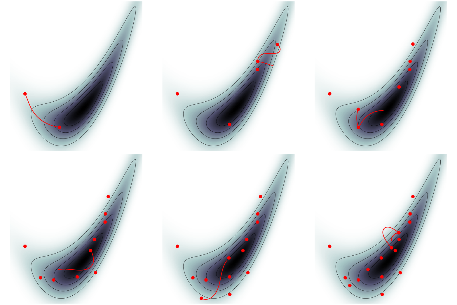
MicroCanonical HMC (Robnik+2022)
Put them to work
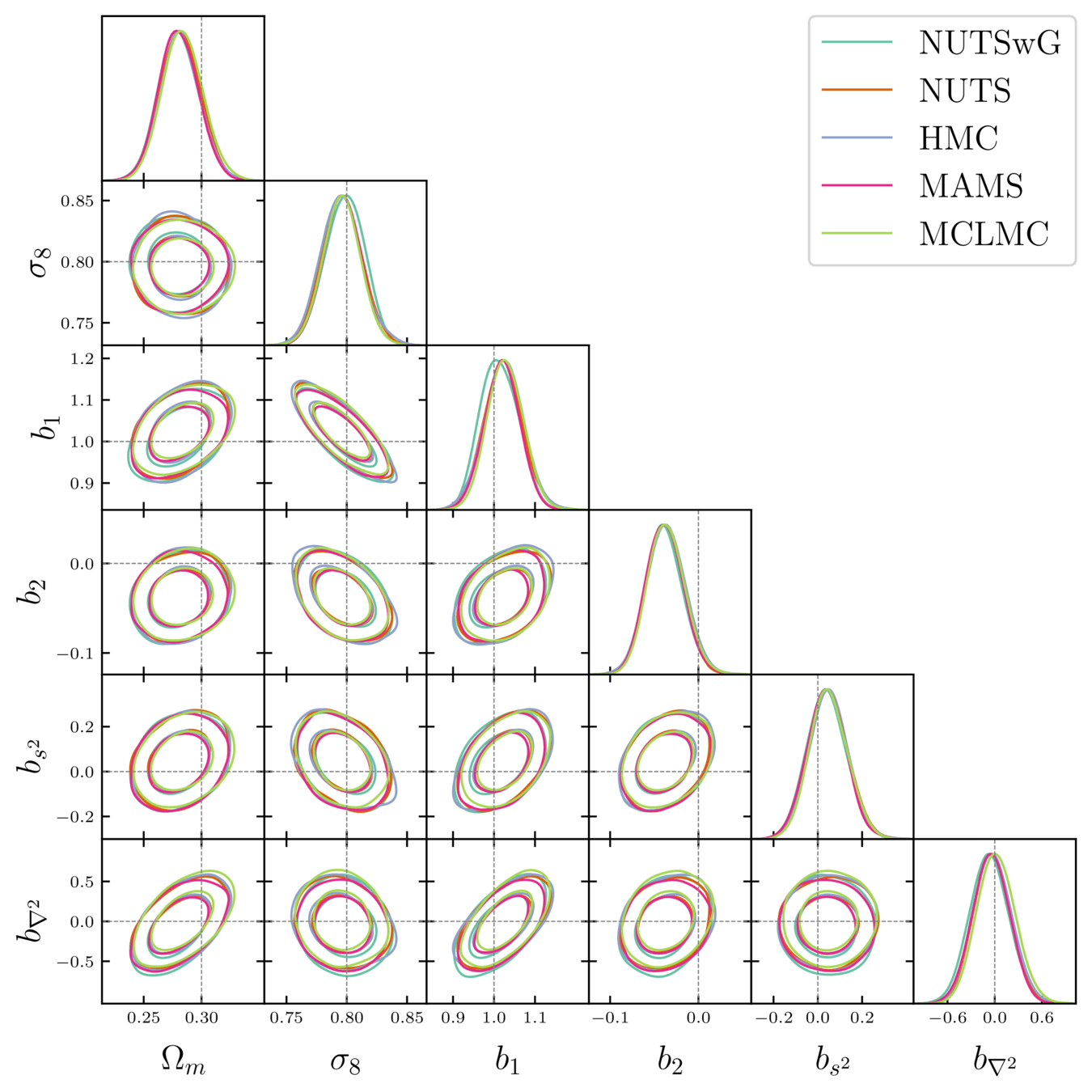
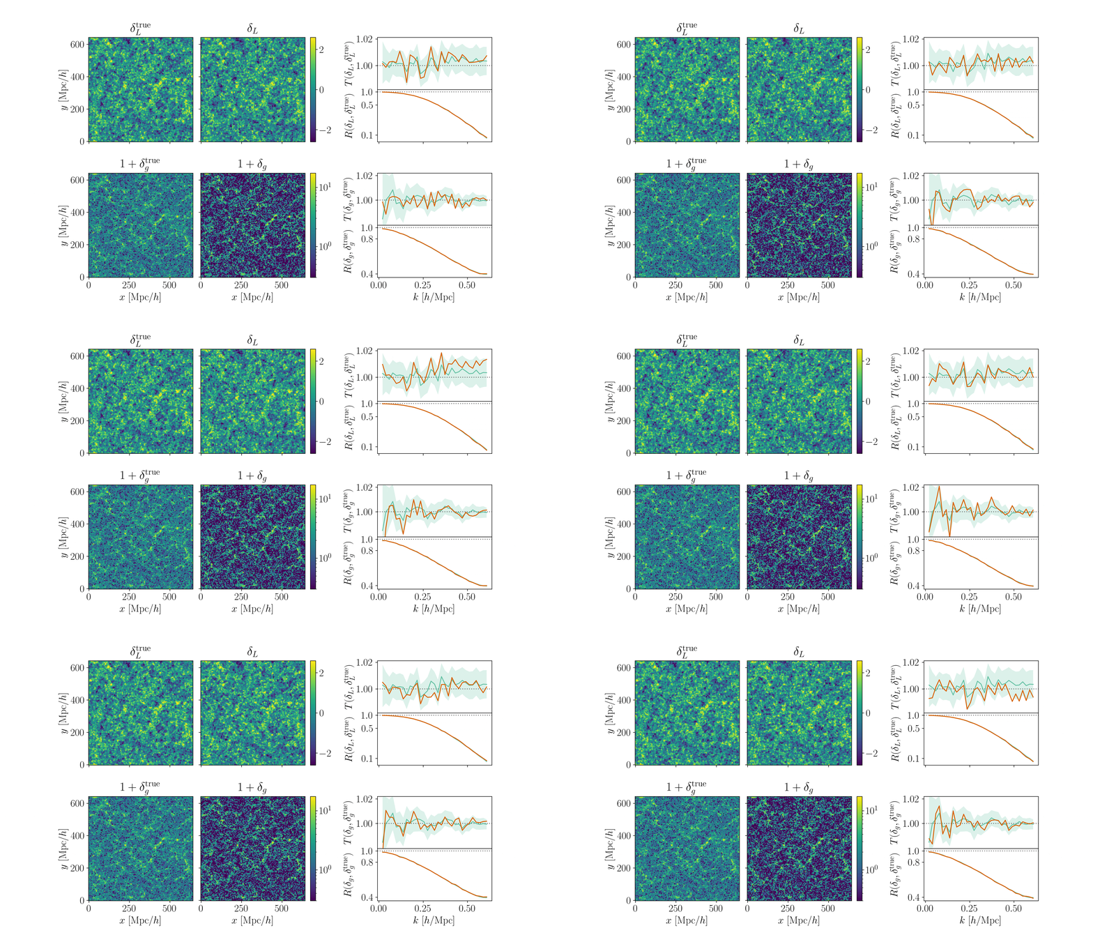
Simon+2025, JCAP
- Multiple samplers and strategies used for FLI in literature:
systematic comparisons required - Evaluate on consistent FLI tasks
Samplers comparison
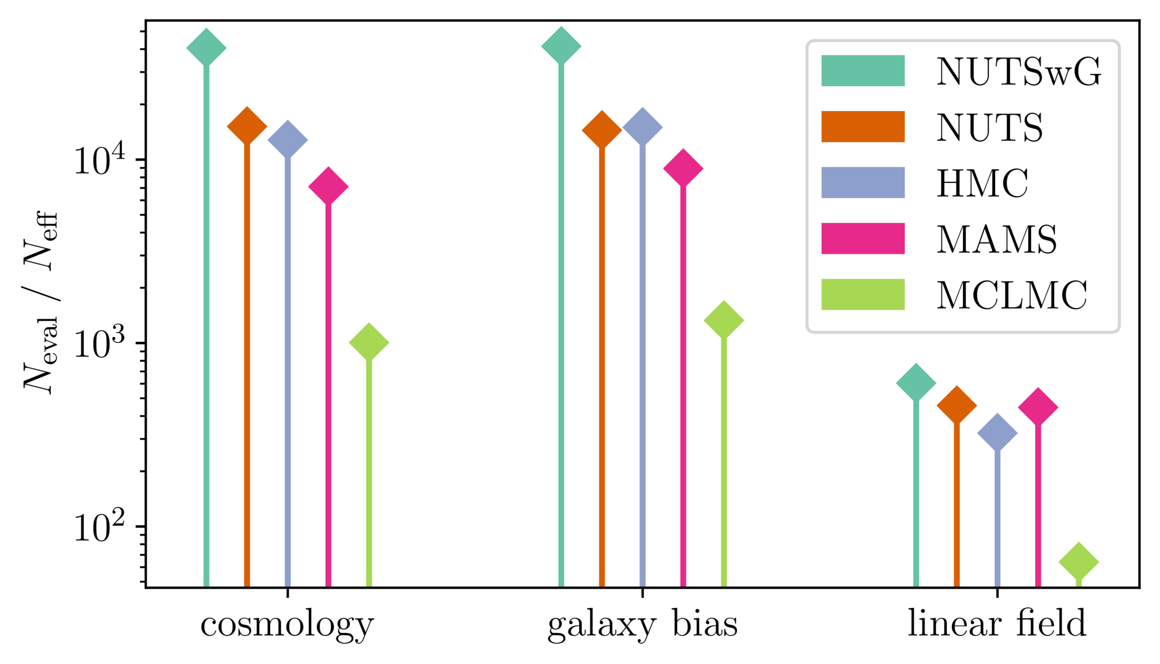
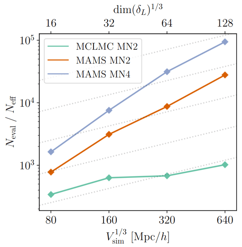
>10 times less evaluations required
flbench, consistent benchmark for field-level from galaxy surveys
unadjusted microcanonical
adjusted microcanonical
adjusted canonical, auto-tuned (NUTS), alternated (within Gibbs)
adjusted sampler
unadjusted sampler
-
microcanonical outperforms canonical
-
unadjusted outperforms adjusted
Model preconditioning
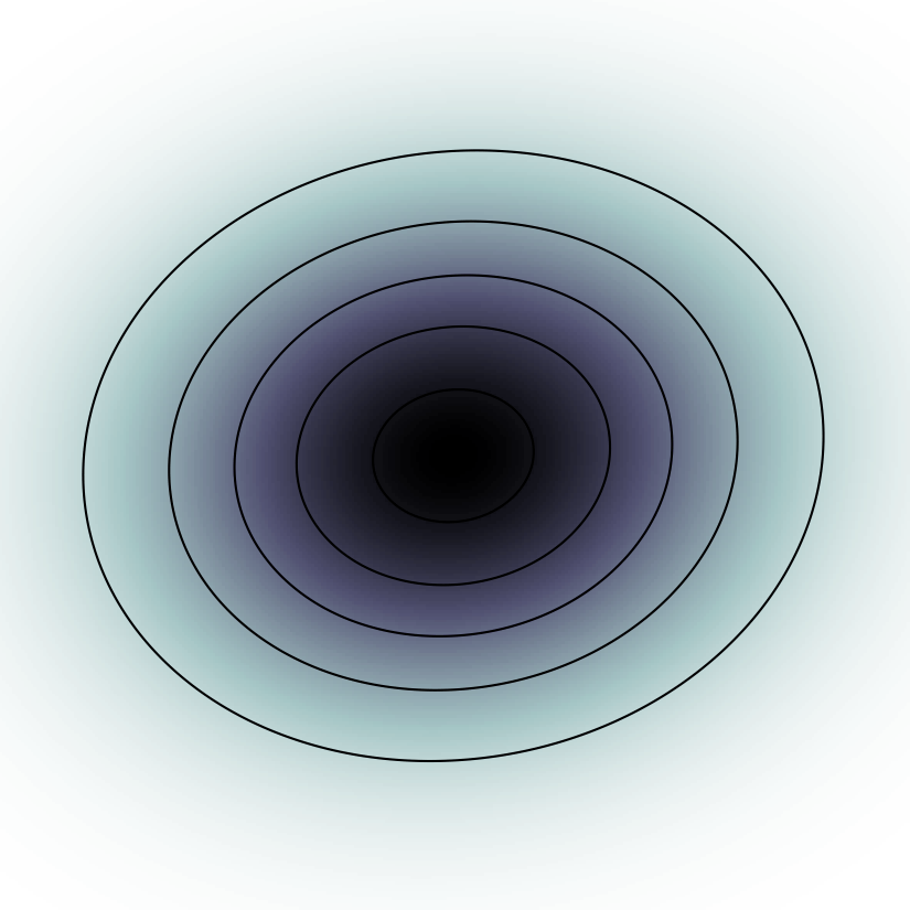
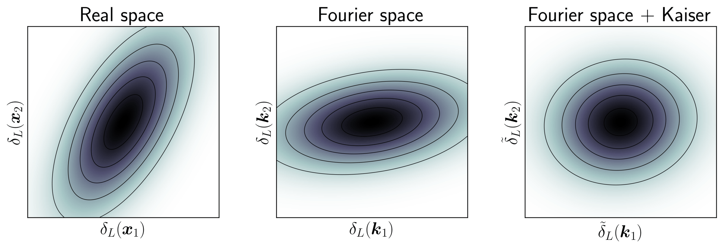
- Sampling is easier when target density is isotropic Gaussian:
- improve acceptance for adjusted methods
- improve bias control for unadjusted methods
- The model is reparametrized assuming a tractable Kaiser model:
linear growth + linear Eulerian bias + flat sky RSD + Gaussian noise
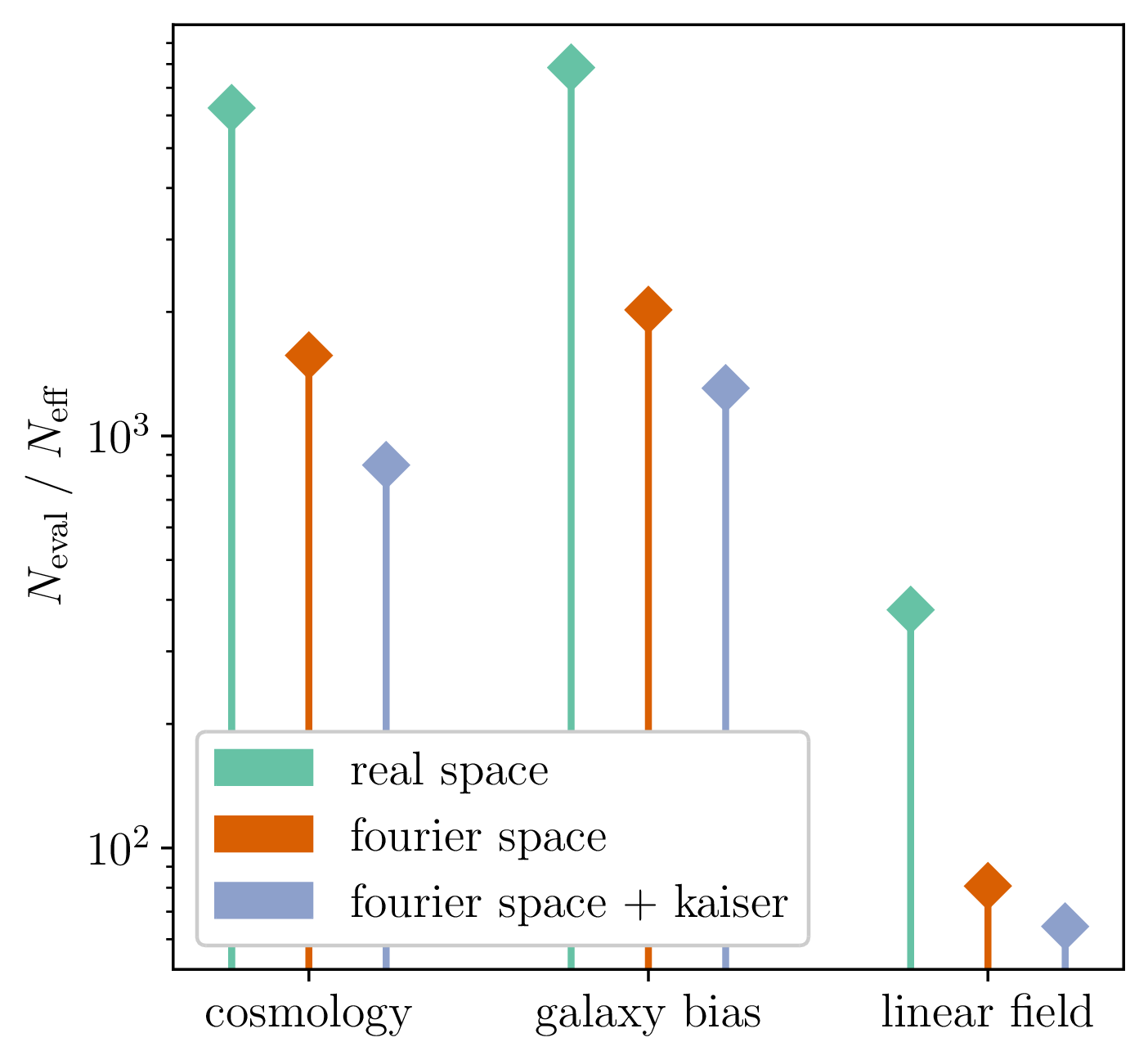
10 times less evaluations required
At the end of the day
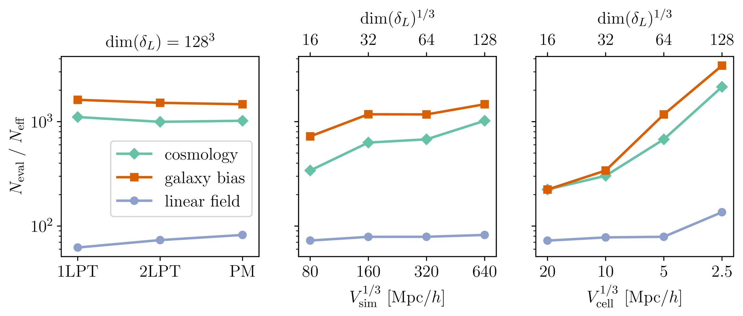
- \(< 10^5\) simulator calls, 4h on a GPU-node for \(128^3\) PM inference (vs. days!)
- Promising for future inferences, going multi-GPU
Mildly dependent with respect to formation model and volume
Probing smaller scales could be harder
MCLMC sampler + field-level preconditioning:
Probing the Inflation at the Field Level
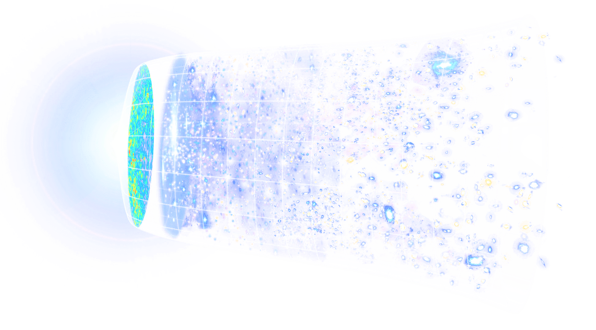
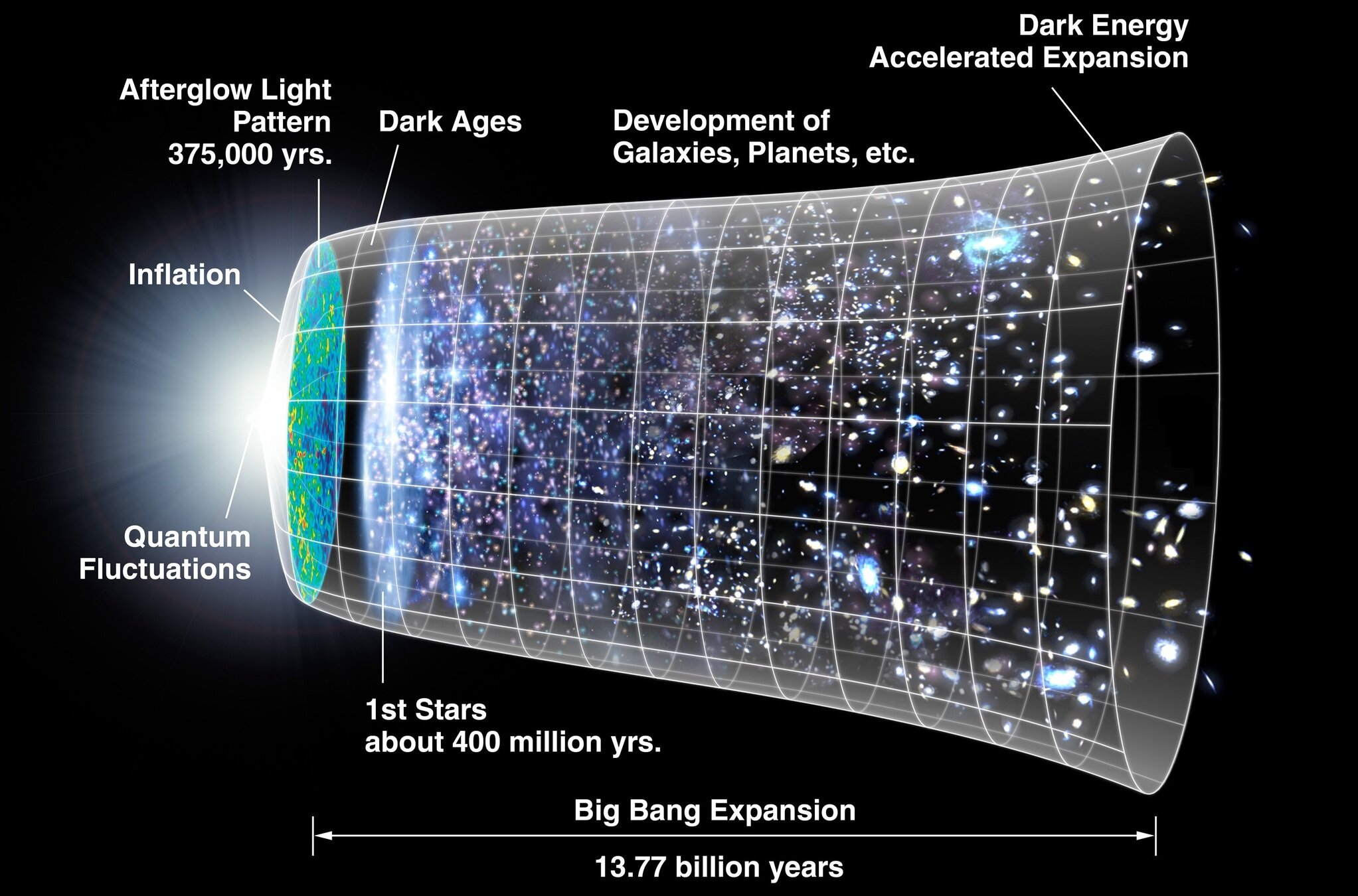
- Fast expansion explaining Universe homogeneity, flatness, and initial perturbations
- Simplest model is single-field slow roll inflation
- But other models exist, that we need to discriminate
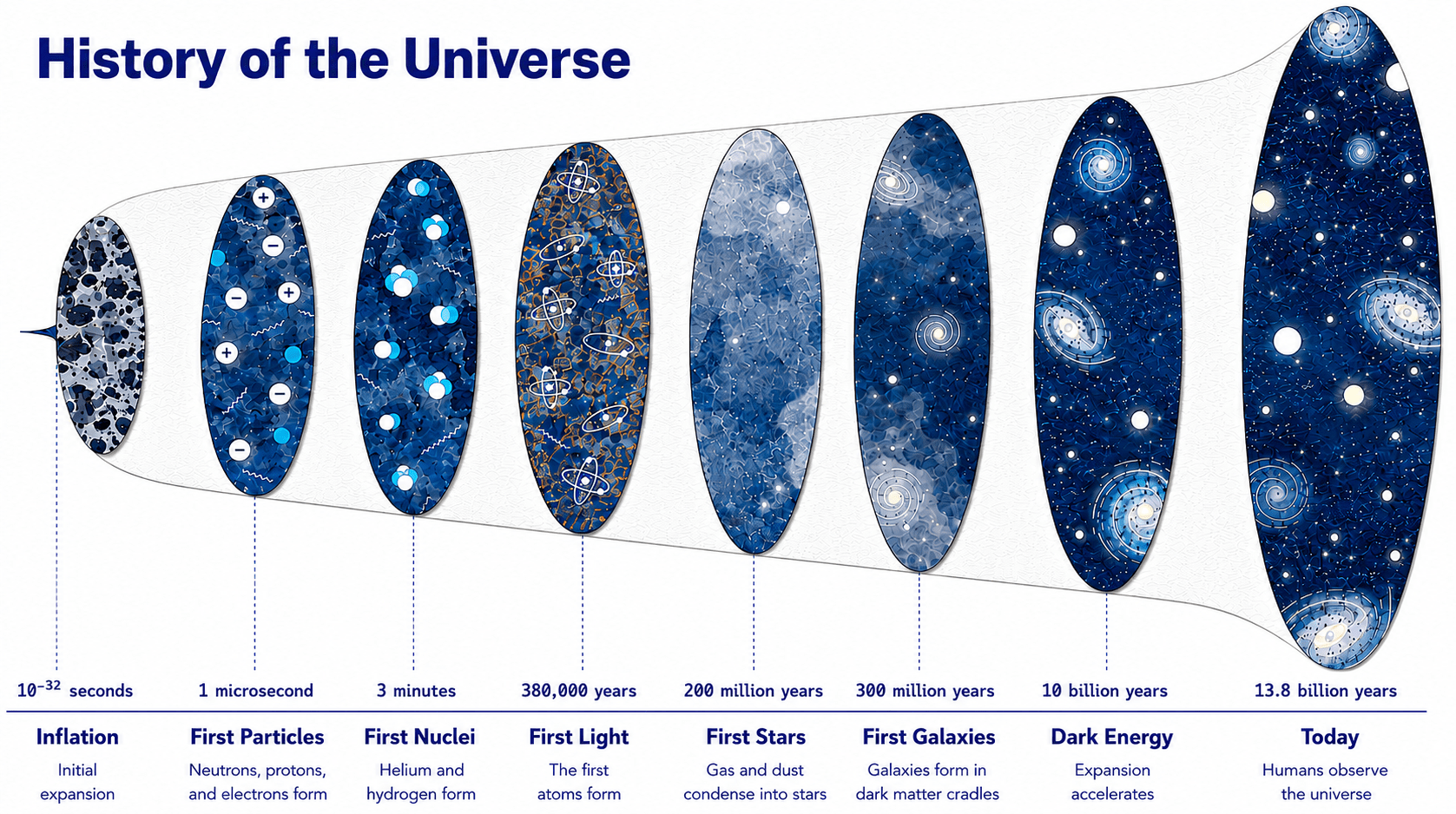
Inspired by NASA and ESA timelines
Local Primordial non-Gaussianity
- Inflation theories discriminated by level of Primordial non-Gaussianity (PNG) predicted. In particular, local PNG quantified by:
$$\phi=\phi_L+{\color{purple}f_{\mathrm{NL}}}\phi_L^{2}$$ - Detecting \(f_\mathrm{NL} \gtrsim 1\) would falsify single-field slow-roll inflation
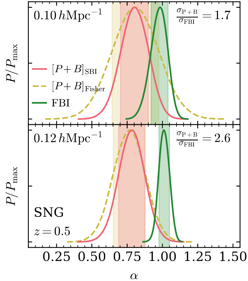
- Current best constraints from CMB bispectrum (Planck+2025): \(f_{\mathrm{NL}}=-0.1\pm 5.0\)
- But there is another way:
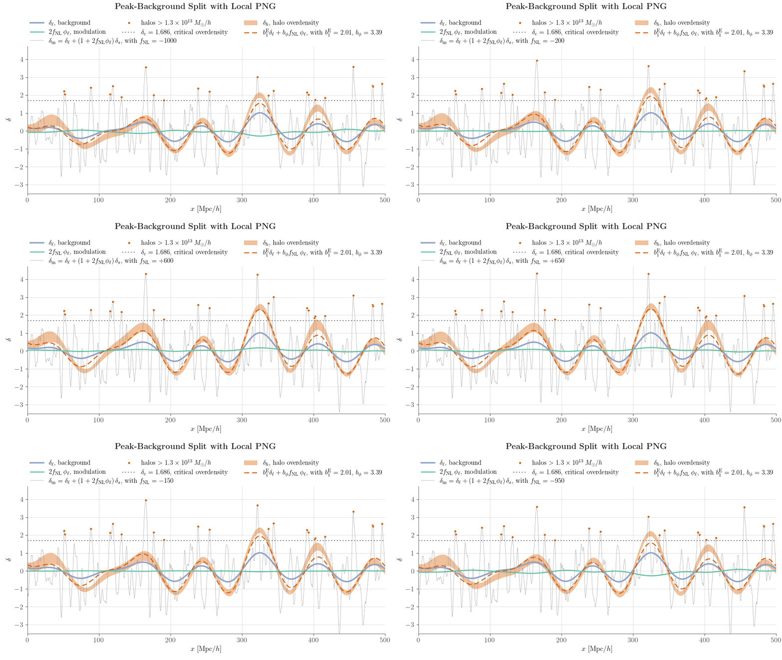
Long-range modulation of short range \(\implies{\color{brown} \delta_g} = b_1^E {\color{blue} \delta_m} + b_\phi {\color{green} f_\mathrm{NL}\phi_L} \)
Probing inflation with galaxies
Ideal demonstration for FLI
- Most of signal from easier large scales
- Result sensitive to survey selection and systematics, more directly implemented and inspected at field-level
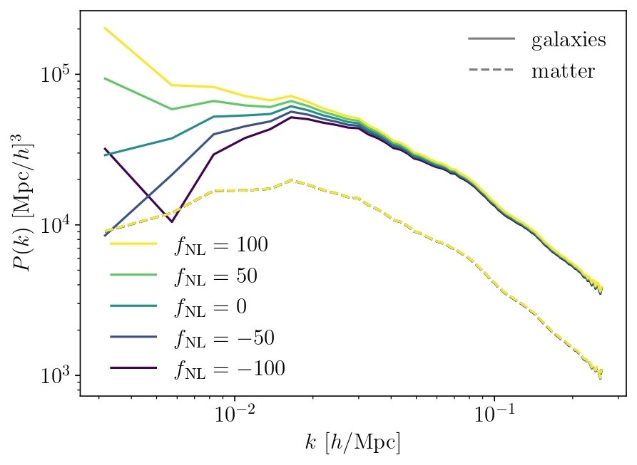
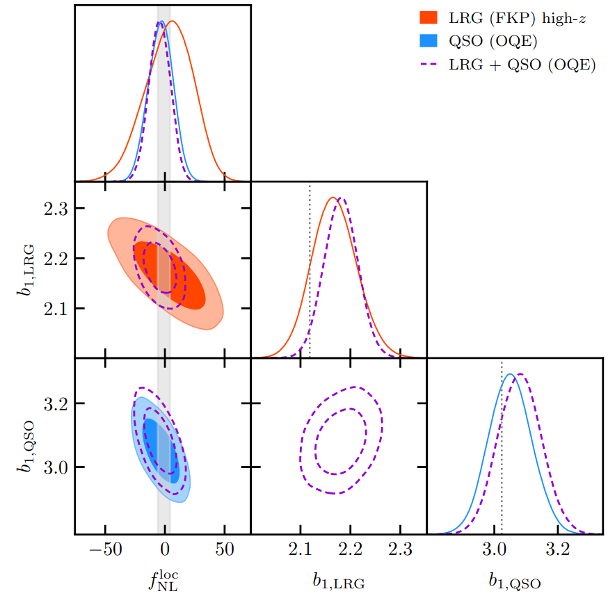
- Therefore$$\begin{align*} \delta_g(\boldsymbol{k}) &\simeq b_{1}\,\delta_L(\boldsymbol{k}) + b_\phi\,{\color{purple}f_\mathrm{NL}}\,\phi_L(\boldsymbol{k}) \\ & \simeq \left(b_{1} + \tilde b_\phi\,{\color{purple}f_\mathrm{NL}}\,k^{-2}\right)\delta_L(\boldsymbol{k})\end{align*}$$a scale-dependent bias
- From DESI DR1 LRG and QSO galaxy power spectrum:$$f_{\mathrm{NL}}=-3.6\pm 9$$
Field-Level modeling of PNG
- Sample initial conditions, add PNG
$$\phi=\phi_L+{\color{purple}f_{\mathrm{NL}}}\phi_L^{2}$$ - Lagrangian EFT 2nd order expansion
$$w_g \supset {\color{purple}f_{\rm NL} b_\phi}\phi_L + {\color{purple} f_{\rm NL} b_{\phi\delta}} \phi_L \delta_{L}$$ - 2LPT evolution and weight particles
- Noise + selection \(W\)
$$n_g \sim \mathcal N({\color{purple}\bar n_g } W(1+\delta_g),\, {\color{purple}\bar n_g }W{\color{purple}s_\varepsilon})$$
3 main PNG contributions,
2 options:
- infer the 3 as independent
- assume "mass relations"
$$\begin{align*}b_\phi &=2\delta_c({\color{purple} b_1}+1-p_\phi)\\b_{\phi \delta} &=2 (\delta_c {\color{purple} b_2}+ {\color{purple} b_1})\end{align*}$$(Lagrangian frame)
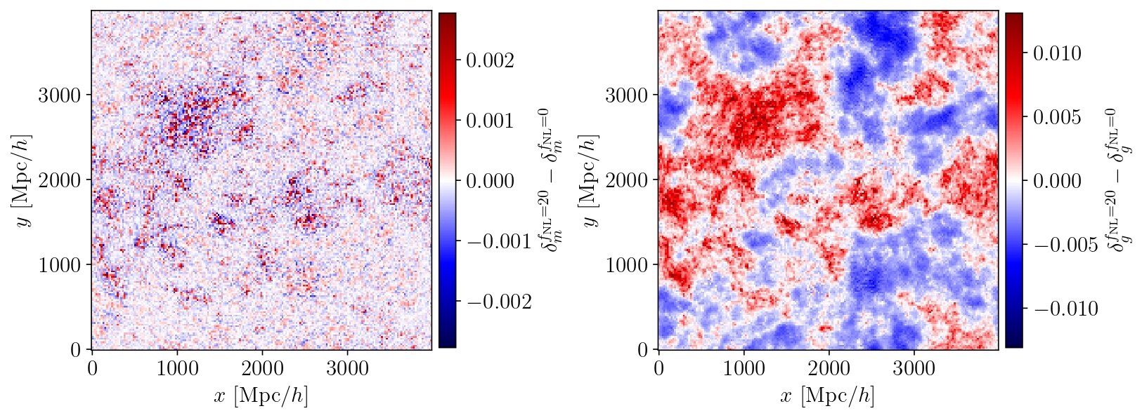
Field-Level Inference of PNG
$$\mathrm{LRG}\, z=0.74$$
$$\mathrm{QSO}\, z=1.83$$
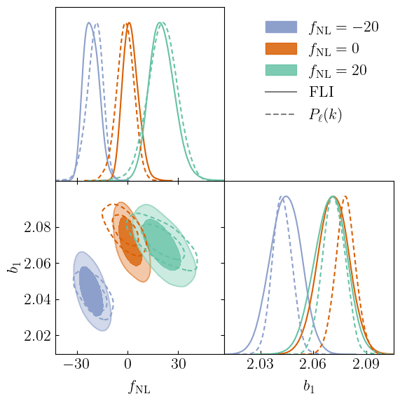
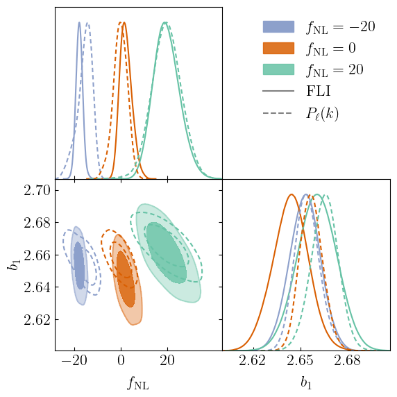
Consistent \(\approx 15 \%\) gain at \(f_\mathrm{NL} = 0\)
DESI reference simulations: PNGUnitsim-XL, largest PNG N-body sims of \((3\ \mathrm{Gpc}/h)^3\)
- \(\textrm{FLI at } k_\mathrm{Nyq} = 0.07\ h/\mathrm{Mpc}\) (\(64^3\), anti-aliasing...)
- \(P_{\{0,2\}}(k) \textrm{ at } k_\mathrm{max} = 0.08 h/\mathrm{Mpc}\)
Recovers \(f_\mathrm{NL}\) and \(b_1\), assuming fitted \(p_\phi\)
Simon+2026 in prep
Toward more survey realism
Example on DESI LRG NGC footprint
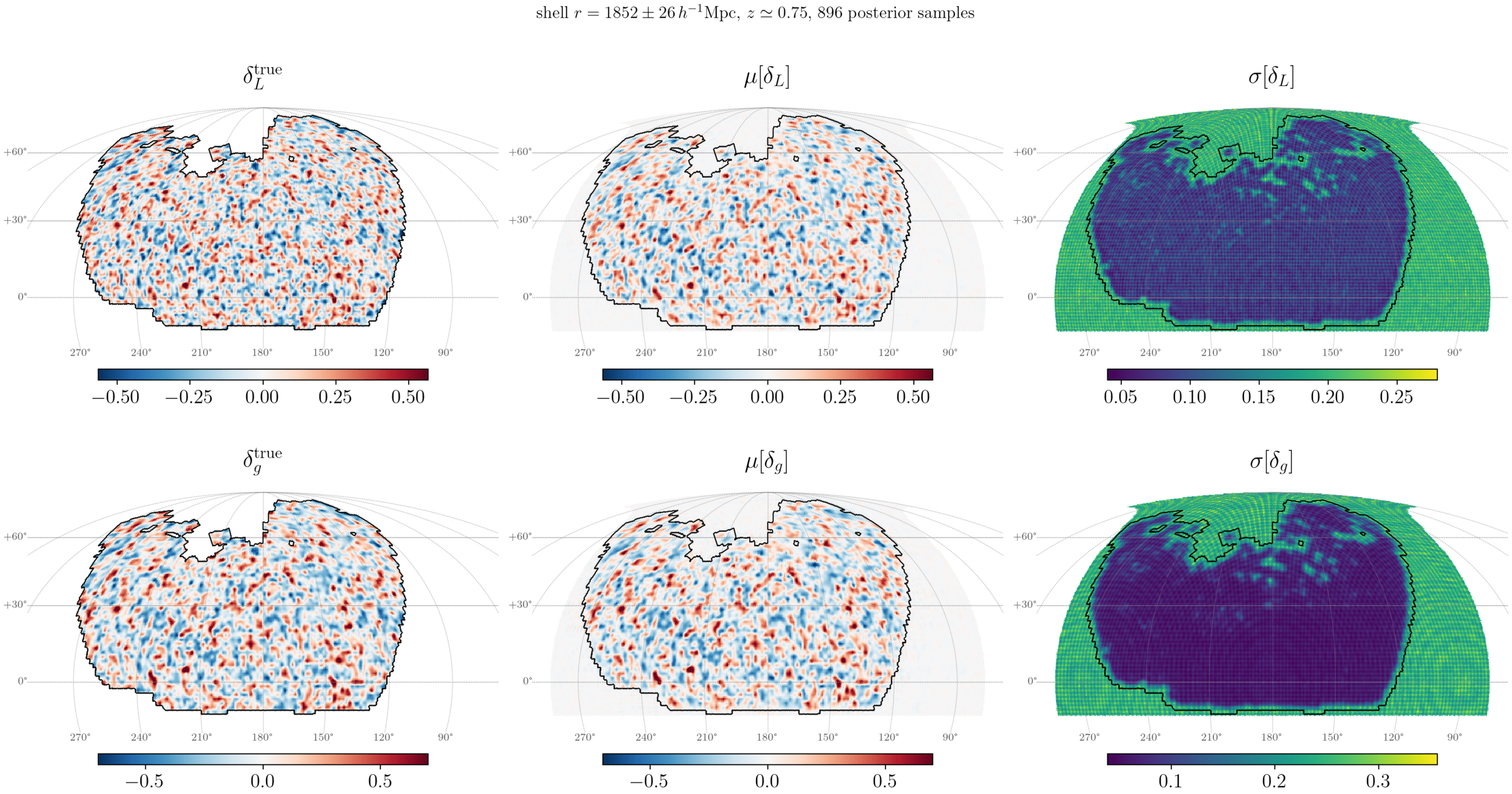
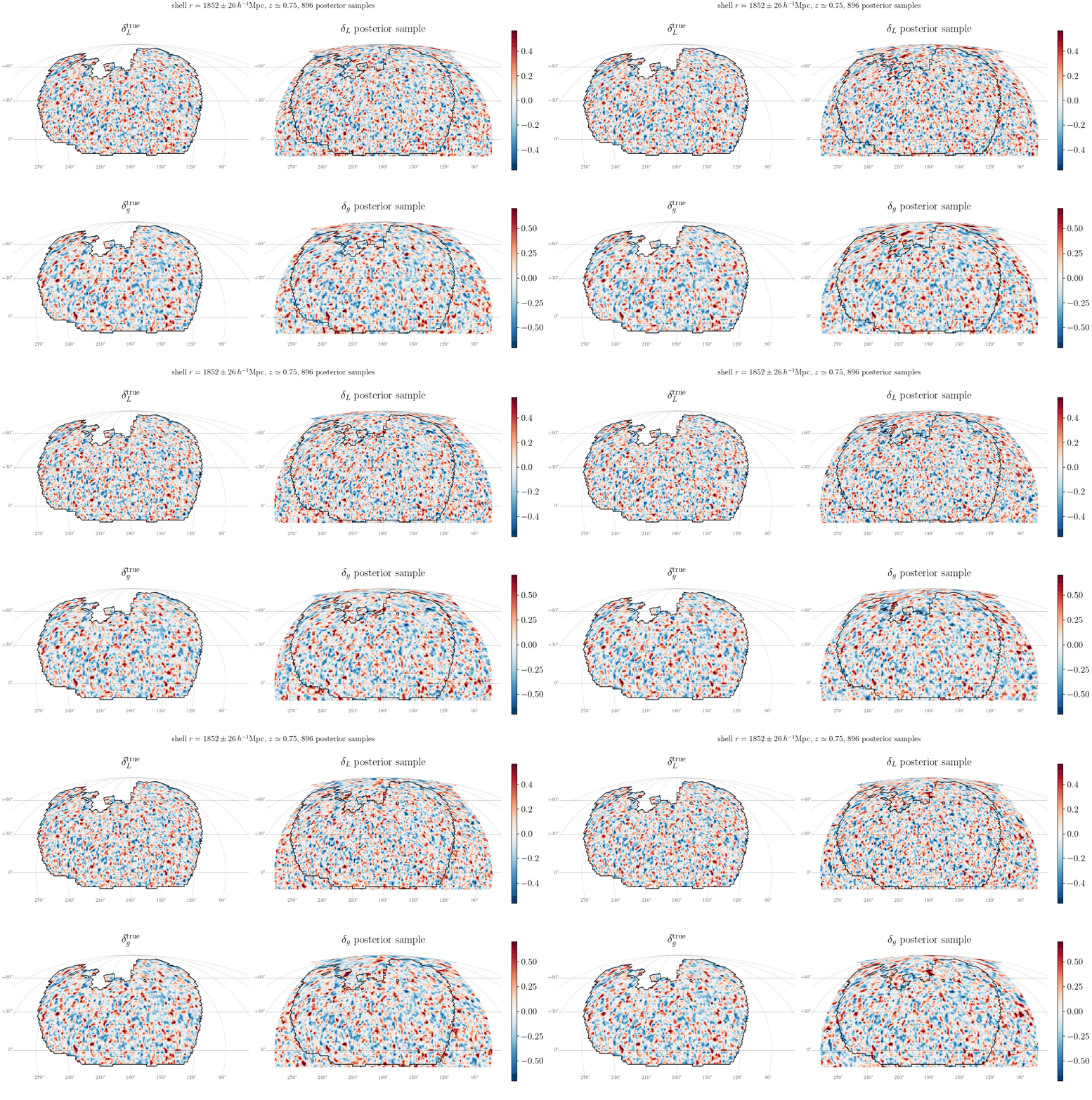
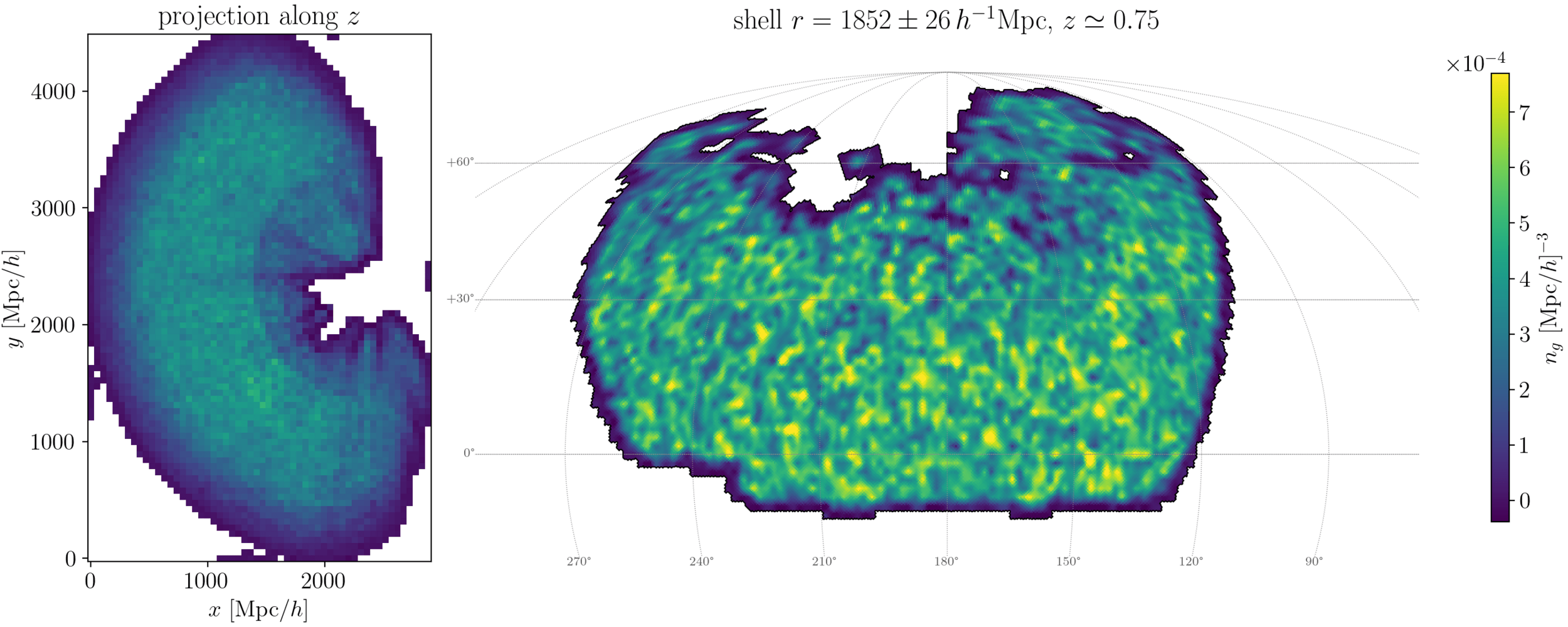
\(k_\mathrm{Nyq} \approx 0.07\, h/\mathrm{Mpc}\)
Constrained inside selection
Prior dominated outside
Toward more survey realism
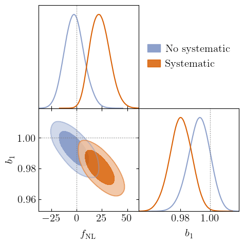
- Inject angular systematic as small localized underdensity, e.g. unmodeled gas cloud
- Thanks to model differentiability, we can ask:
"What are the physical regions that favor a smaller or larger value of \(f_\mathrm{NL}\)?" \(\implies\braket{\nabla_{f_\mathrm{NL}} \log \mathrm p(\boldsymbol x)}\)
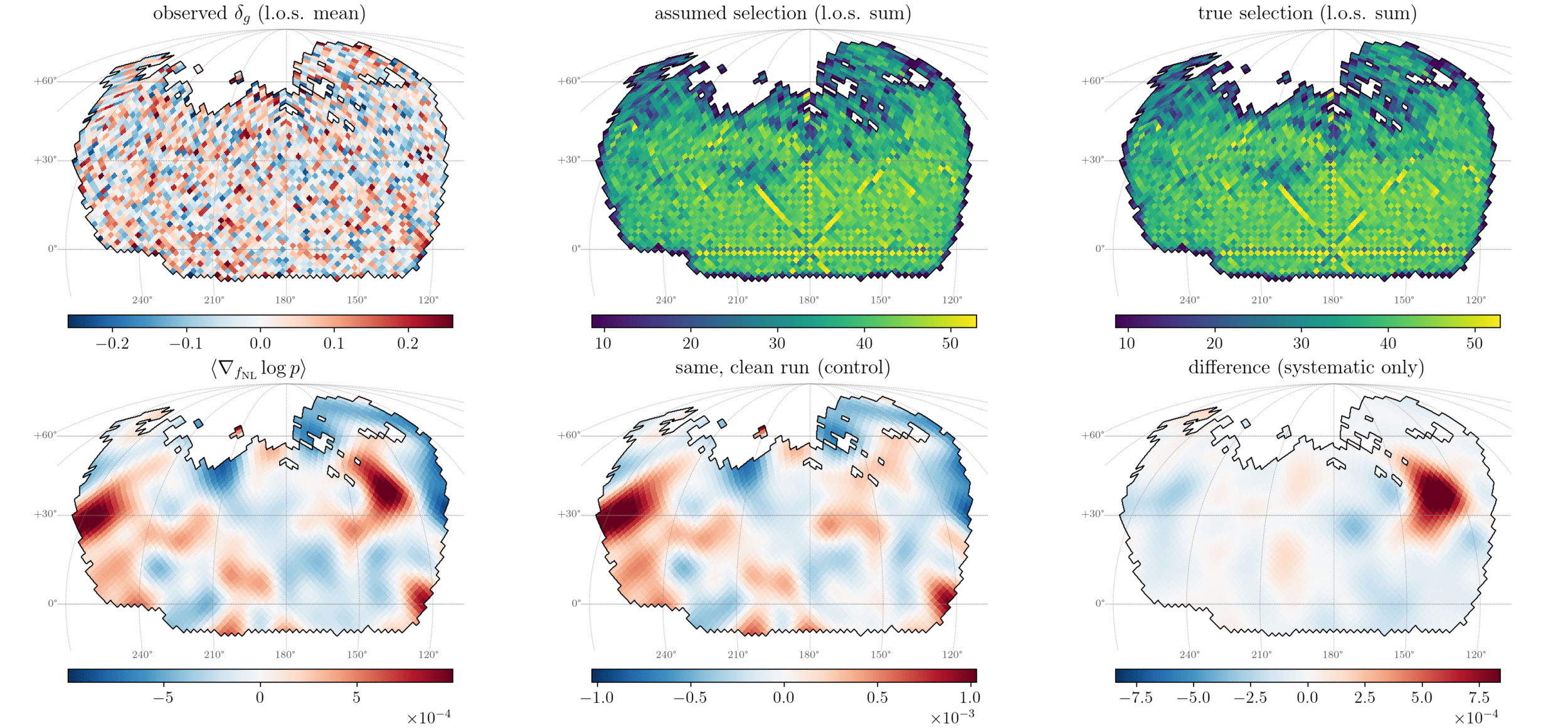
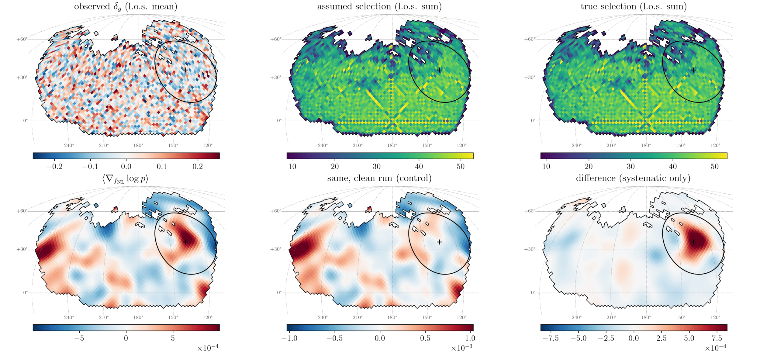
- PNG inference highly sensitive to large scale misspecifications
Simon+2026 in prep
Accessibility \(\implies\) growing community
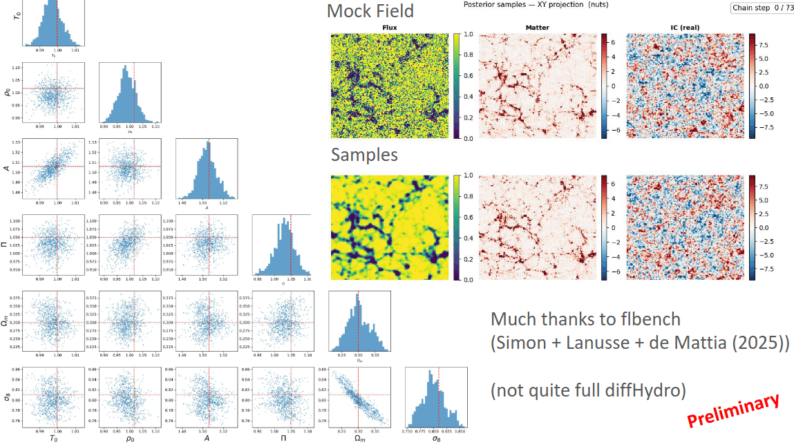
Courtesy of
Ben Horowitz
FLI for Ly\(\alpha\)
PRELIMINARY
In collab with Ethan Smith & Marco Bonici
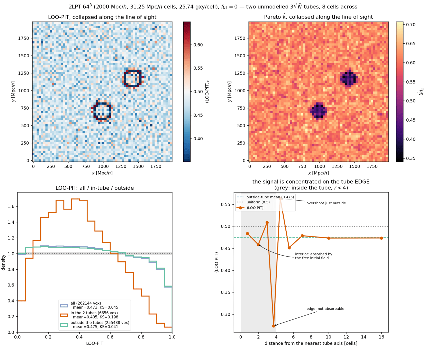
Systematics detection from Leave-One-Out-Probability Integral Transformed (LOO-PIT) field-level posterior
angular syst

Courtesy of
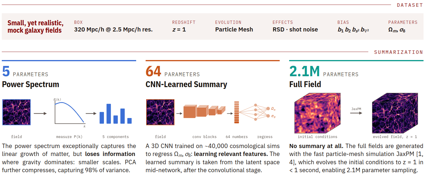
Information content of Higher-Order Statistics vs. Field-Level
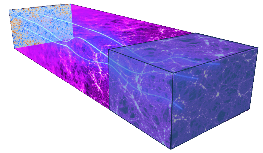
Field-Level Multi-Probing... for CMB lensing
automatically marginalized
simulated volume
Courtesy of Jonathan Hawla
- Extend the current galaxy 3D-field pipeline with CMB lensing convergence 2D-field
- Joint modeling improving constraints:
cross-correlations are automatically taken into account
- Again, fast and differentiable
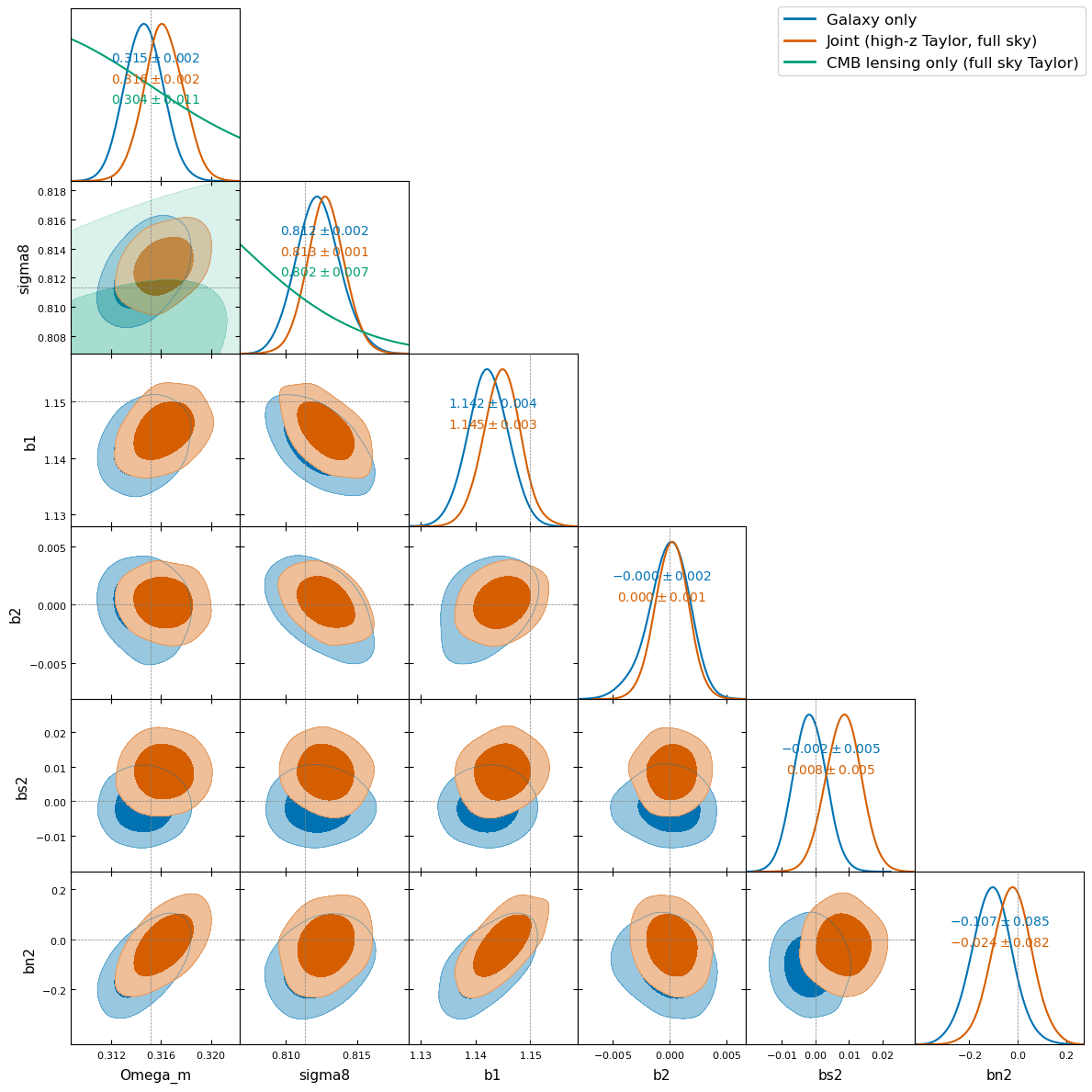
PRELIMINARY- Developed:
- End-to-end FLI pipeline based on differentiable EFT and N-body
- Benchmark and sampling strategies making FLI scalable to current and future surveys
- Validation on high-fidelity simulations against standard analysis,
paving the way to application on PNG inference from DESI
- Continue working on:
- Multi-tracer, then multi-probe
- Detection of unmodeled systematics
- Improve numerical efficiency, e.g. with diffusion model
Conclusion & Prospects
Thank you!
From summary stat inference...
\(s\)
\(s\)
\(\delta_L\)
\(\Omega\)
\(\delta_g\)
\(\Omega := \{ \Omega_m, \Omega_\Lambda, H_0, \sigma_8, f_\mathrm{NL},...\}\)
- Whole Universe map \(\delta_g\) compressed into summary stat \(s\)
From summary stat inference...
\(s\)
\(s\)
\(\delta_L\)
\(\Omega\)
\(\delta_g\)
\(\Omega := \{ \Omega_m, \Omega_\Lambda, H_0, \sigma_8, f_\mathrm{NL},...\}\)
\(s\)
\(s\)
\(\Omega\)
inference
- Whole Universe map \(\delta_g\) compressed into summary stat \(s\)
- Marginalize, then sample \(\Omega \mid s\)
- \(s\) more simple \(\implies\) lossier compression
- \(s\) more complex \(\implies\) less tractable marginalization
Field-Level Inference
\(\delta_L\)
\(\Omega\)
\(\delta_g\)
\(\Omega := \{ \Omega_m, \Omega_\Lambda, H_0, \sigma_8, f_\mathrm{NL},...\}\)
\(\delta_g\)
\(\delta_L\)
\(\Omega\)
inference
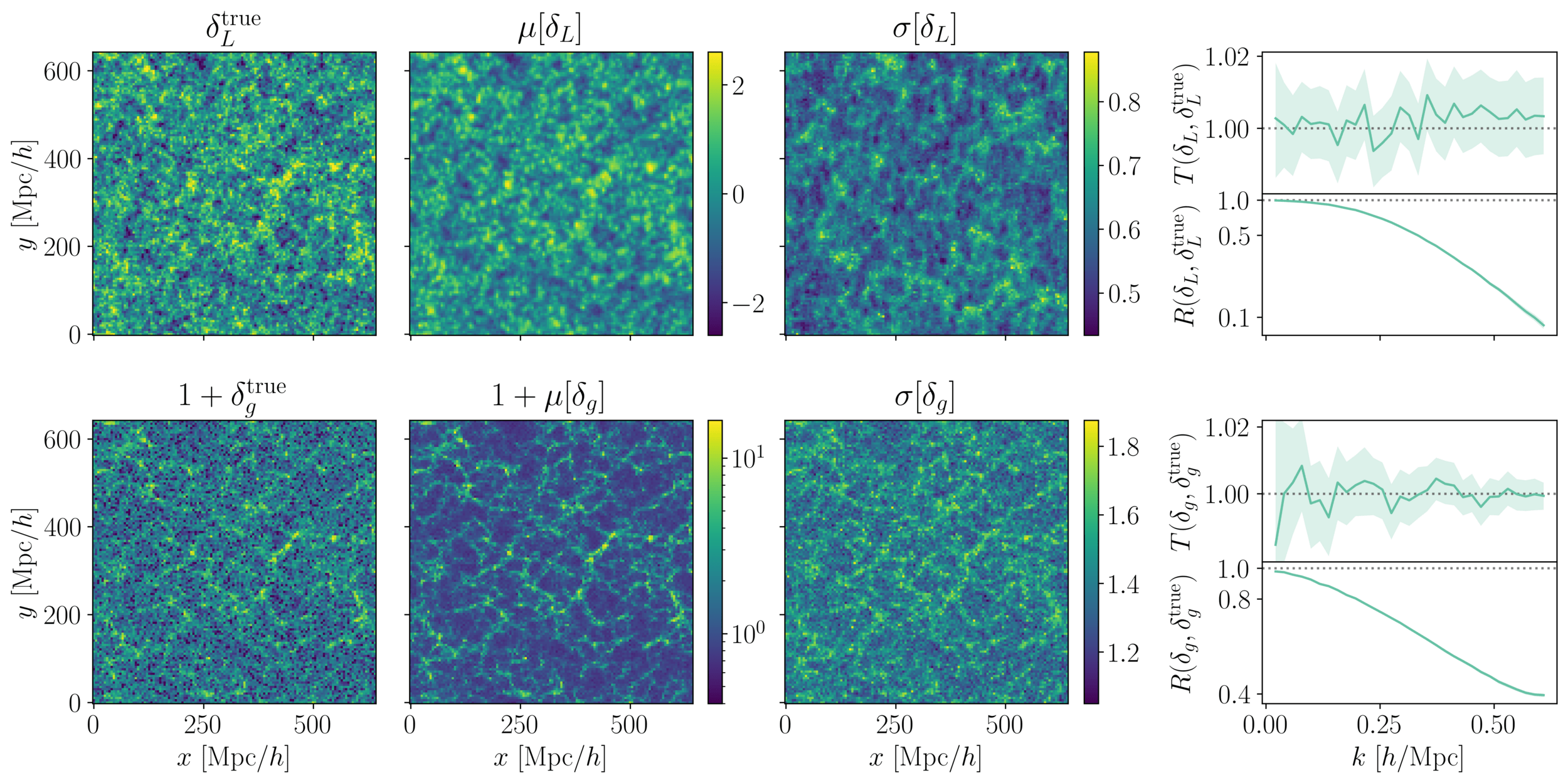
- Infer the cosmology and reconstruct the initial conditions, by sampling directly \(\Omega, \delta_L \mid \delta_g\)
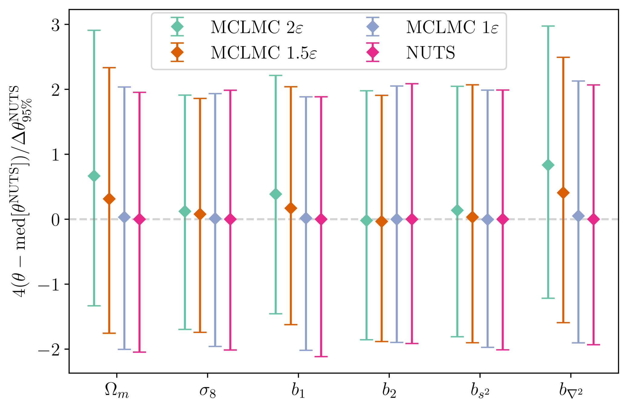
Afraid of unadjusted sampling?
- Microcanonical dynamics \(\implies\) energy should not vary
- Numerical integration yields quantifiable errors that can be linked to bias
see e.g. Robnik+2024 - Reducing stepsize rapidly brings bias under Monte Carlo error
-
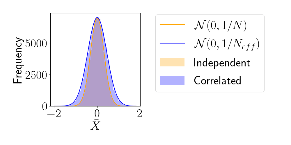
Effective Sample Size (ESS)
- number of i.i.d. samples that yield same statistical power.
- For sample sequence of size \(N\) and autocorrelation \(\rho\) $$N_\textrm{eff} = \frac{N}{1+2 \sum_{t=1}^{+\infty}\rho_t}$$so aim for as less correlated sample as possible.
- Main limiting computational factor is model evaluation (e.g. N-body), so characterize MCMC efficiency by \(N_\text{eval} / N_\text{eff}\)
How to compare samplers?
Put them to work
- Multiple samplers and strategies used for FLI in literature:
systematic comparisons required - Evaluate on consistent FLI tasks
$$\sqrt{P_{\delta} / P_{\delta^\mathrm{true}}}$$ \(\approx\) amplitude info
$$P_{\delta,\delta^\mathrm{true}} / \sqrt{P_{\delta}P_{\delta^\mathrm{true}}}$$ \(\approx\) phase info
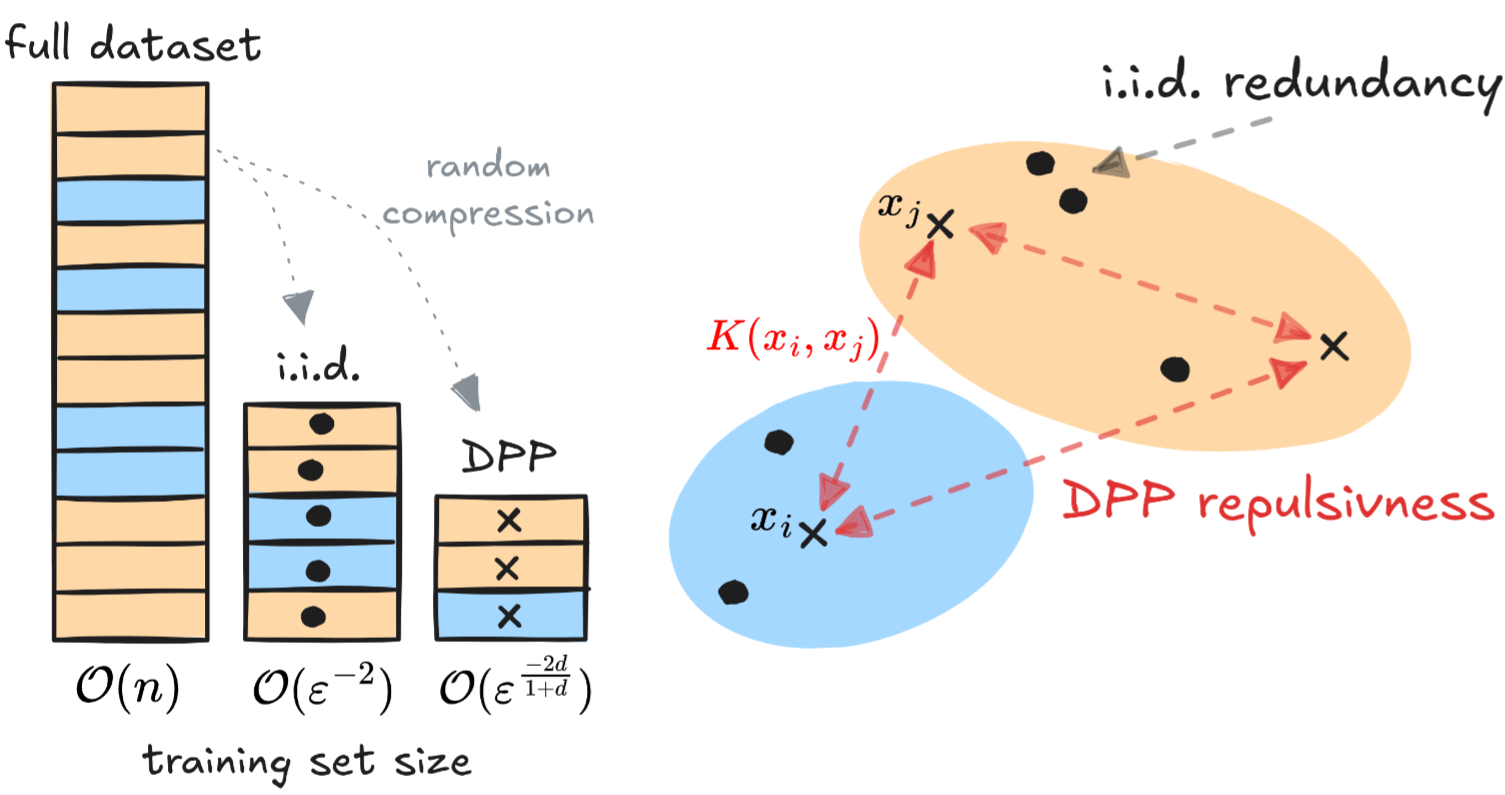
Low-dimensional sampling is simple
- Can beat the \(n^{-1/2}\) rate in low dimension
- Applied to \(k\)-means problems and accepted to NeurIPS-2024 as spotlight paper
Field-level inference
Summary stat inference
\(\Omega\)
\(s\)
\(\delta_g\)
\(\Omega\)
\(\delta_L\)
\(s\)
marginalize
condition
marginalize
\(\Omega\)
\(s\)
\(\delta_g\)
\(\Omega\)
\(\delta_L\)
condition
Two approaches to cosmological inference
Cosmo model
\(\mathrm{p}(\Omega,s)\)
\(\mathrm{p}(\Omega \mid s)\)
\(\Omega\)
\(\delta_g\)
\(\mathrm{p}(\Omega,\delta_L,\delta_g, s)= \mathrm{p}(s \mid \delta_g) \, \mathrm{p}(\delta_g \mid \Omega,\delta_L)\, \mathrm{p}(\delta_L \mid \Omega)\, \mathrm{p}(\Omega)\)
\(\mathrm{p}(\Omega,\delta_L \mid \delta_g)\)
\(\mathrm{p}(\Omega \mid \delta_g)\)
\(\delta_g\)
\(\Omega\)
\(\delta_L\)
\(s\)
Two approaches to cosmological inference
Cosmo model
Problem:
- \(s\) is too simple \(\implies\) lossy compression
- \(s\) is too complex \(\implies\) intractable marginalization
The Problem:
- high-dimensional integral $$\mathrm{p}(\Omega \mid \delta_g) = \int \mathrm{p}(\Omega, \delta_L \mid \delta_g) \;\mathrm d \delta_L$$
- To probe scales of \(15\ \mathrm{Mpc}/h\) in DESI volume, \(\operatorname{dim}(\delta_L) \simeq 1024^3\)
The Promise:
- "lossless" explicit inference
Field-level inference
Summary stat inference
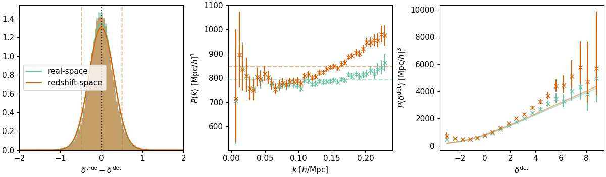
Galaxy stochasticity
\({\color{purple}\sigma_0}|1+{\color{purple}\sigma_\delta}\delta_g^\mathrm{det}|\)
Poisson \(\simeq \sigma_0=\sigma_\delta=1\), but fits show sub-Poisson
\(k_\mathrm{nyq} \leq 0.15 h/ \mathrm{Mpc}\)
\(\delta_g \sim \mathcal N(\delta_g^\mathrm{det},\, {\color{purple}❓})\)
\({\color{purple}\sigma_0}(1+{\color{purple}\sigma_{2}}k^2 + {\color{purple}\sigma_{\mu,2}}(\mu k)^2)\)
Negligible for currently probed scales.
Galaxy stochasticity = \(\delta_g^\mathrm{true} -\delta_g^\mathrm{det}\), and we take \(\delta_g^\mathrm{det}\) to be EFT best fit.
\(\sigma^2(\delta^\mathrm{det})\)
Fitting AbacusSummit+HOD
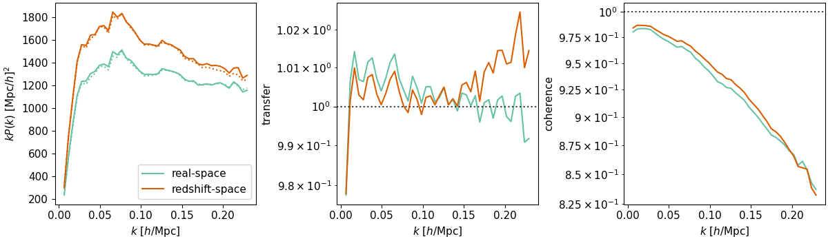
- Matter: fix initial conditions. Match within \(0.5\%\) at field-level for \(k_\mathrm{nyq} < 0.1 h/\mathrm{Mpc} \)
- Tracer (LRG, \(z=0.8\)): fix initial conditions and optimize on EFT parameters
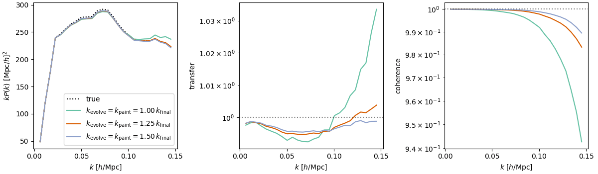
$$\sqrt{P_{\delta} / P_{\delta^\mathrm{true}}}$$ = amplitude info
$$P_{\delta,\delta^\mathrm{true}} / \sqrt{P_{\delta}P_{\delta^\mathrm{true}}}$$ = phase info

Foutus Mocks!
Thank you!


Thank you!

PS: \(k_\mathrm{Nyq} = \pi / l_\mathrm{cell}\)
Thank you!

2026Defense
By hsimonfroy