


He Wang PRO
Knowledge increases by sharing but not by saving.
2025/12/18, MLA call
He Wang
hewang@ucas.ac.cn
University of Chinese Academy of Sciences (UCAS)
On behalf of the KAGRA collaborations
based on 2024 Mach. Learn.: Sci. Technol. 5 015046
(arxiv: 2212.14283)
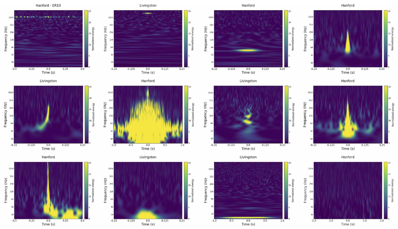
1400Ripples Air Compressor Blip
Extremely Loud Helix Koi Fish
Various types of Glitch
The improvement of data quality is a very complex issue, with data from over 20,000 sensor channels determining the quality of the gravitational wave science data channel.
Reducing non-Gaussian short-duration pulse interference (Glitches) in gravitational wave data will help reduce the false alarm rate of gravitational wave signals.
Removing Glitches from gravitational wave detection data is a multi-classification problem.
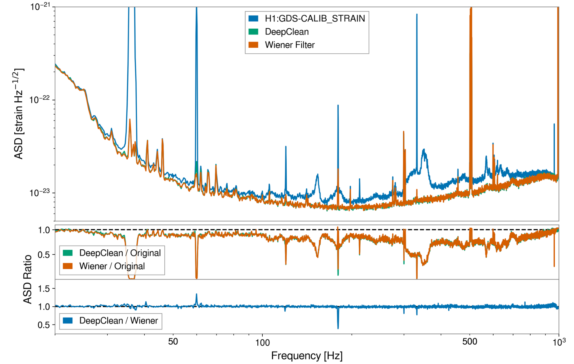
Ormiston R, et al. PRR, 2020
DeepClean: One-dimensional Convolutional Neural Network which takes a specified set of witness channels and subsequently outputs the predicted noise in strain.
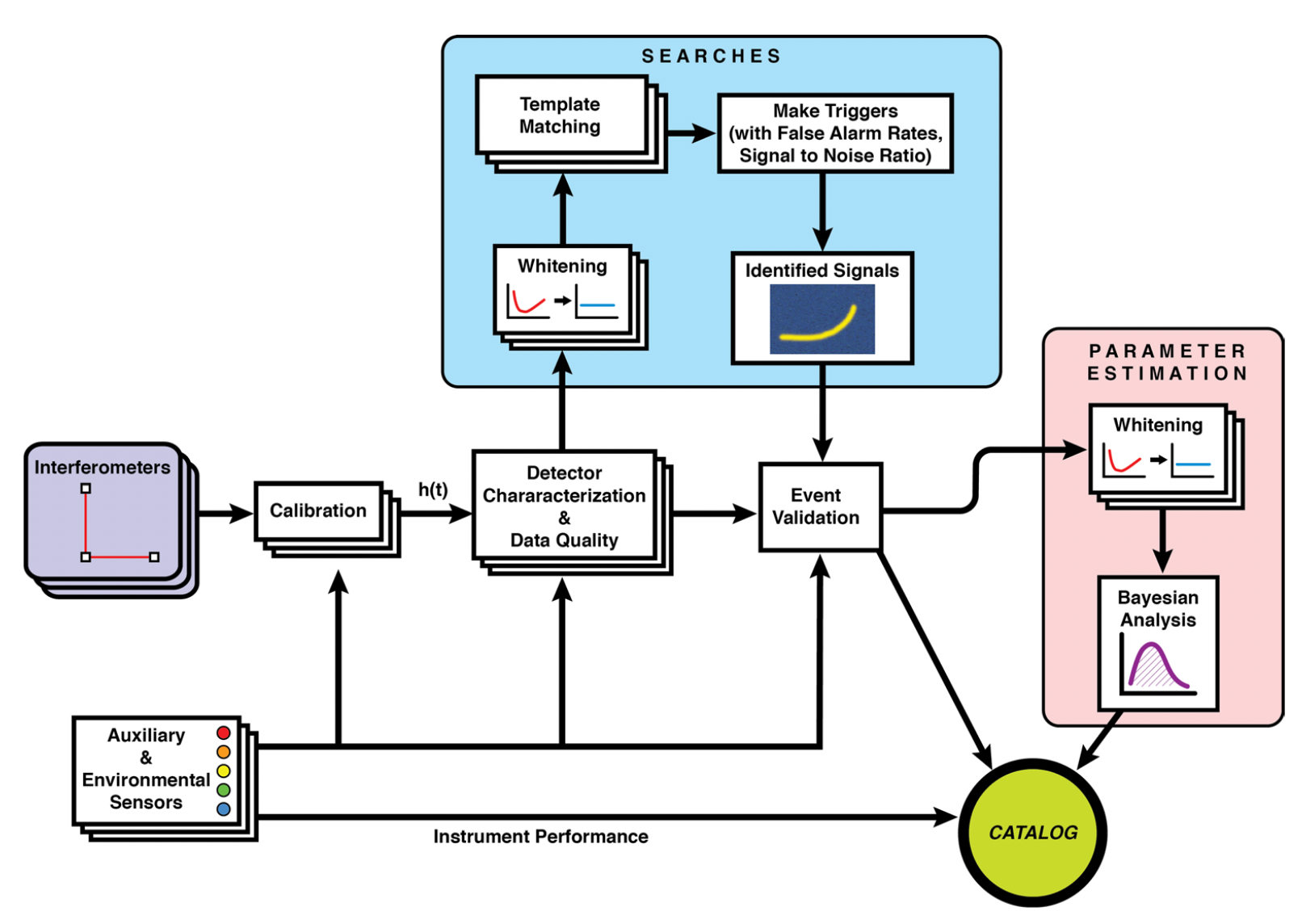
IGWN data processing
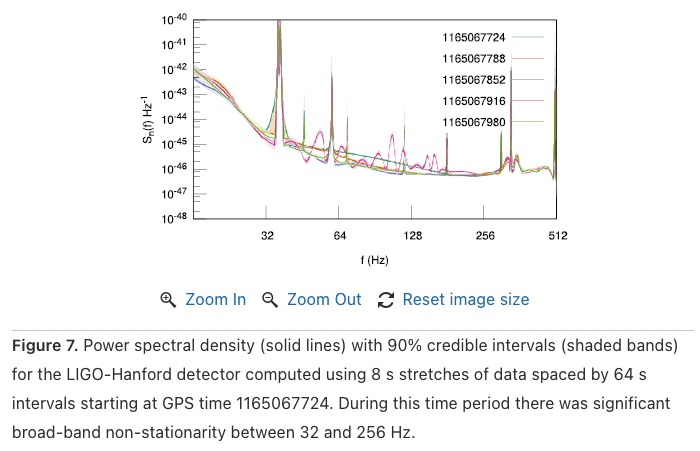
Non-stationary
Non-Gaussianity
Background
Related Works
Model Structure
Precessing & Train
Effect on Noise
Effect on BBH signals
Credit: Marco Cavaglià
Chatterjee C, Wen L, et al. PRD 2021
Wei W and Huerta E A. PLB 2020
Bacon P. et al. MLST 2023
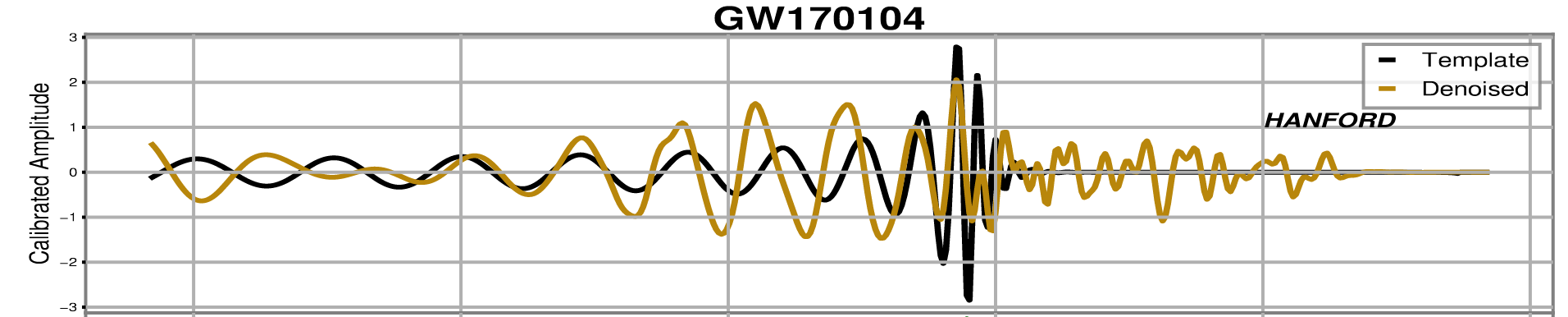
GW170823
Murali C & Lumley D. PRD 2023
["This", "is", "a", "sample"]
[1, 16512]
[1, 128, 256]
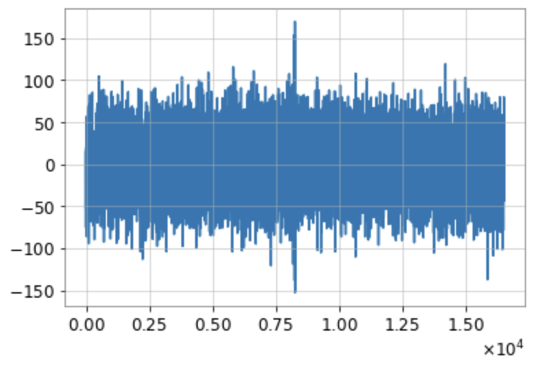
Given �=ℎ+�d=h+n, we can normalize �d as follows:
Strain
Whiten
Normalized
∼\(10^{−19}\)
∼\(10^{2}\)
∼\(10^{0}\)
32 s
32 s
merger
\(t_c\) (e.g. near GW150914)
Band-pass: [20, 2048] Hz
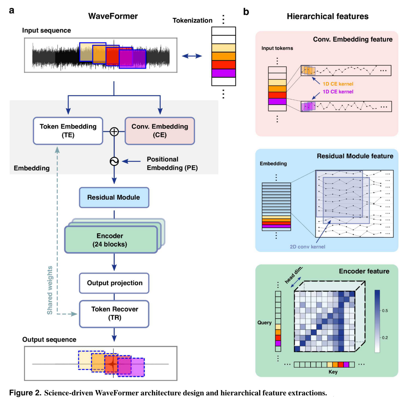
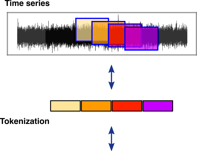
Patching (tokenized) with size 0.125 s and overlap 50%
[1, 128, 256]
(Standard normalization)
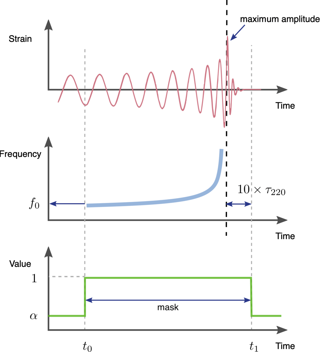
dynamic masking
[1, 16512]
[1, 128, 256]
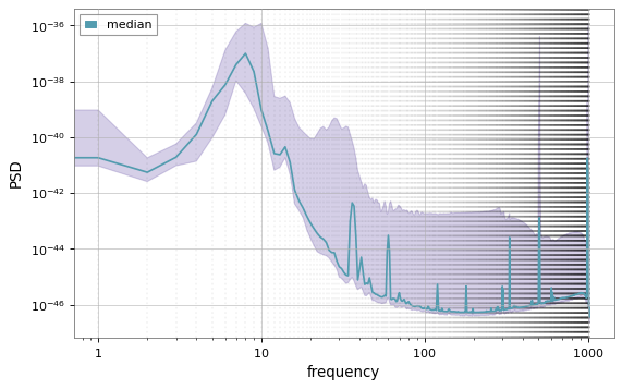
(PSD\(_i\) from noise)
Band-pass: [20, 2048] Hz
WaveFormer
MSE-Loss\(_i\)
\(std\)
[1, 128, 256]
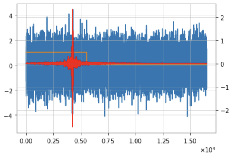
Noise\(_i\):
Signal\(_i\):
Input\(_i\):
Label\(_i\):
Output\(_i\):
8.0625 s
8.0625 s
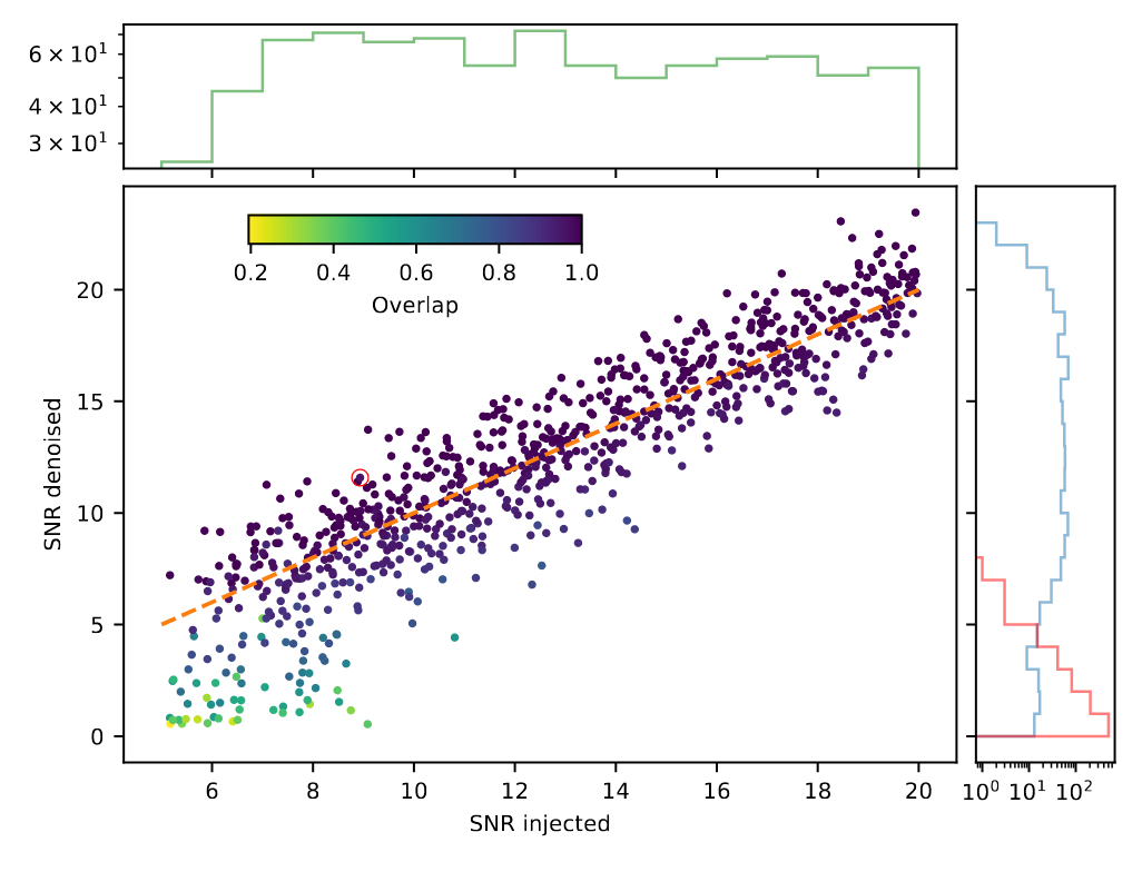
(Cal. network SNR)
Given �=ℎ+�d=h+n, we can normalize �d as follows:
Strain
Whiten
Normalized
∼\(10^{−19}\)
∼\(10^{2}\)
∼\(10^{0}\)
32 s
32 s
merger
\(t_c\) (e.g. near GW150914)
(Cal. network SNR)
Band-pass: [20, 2048] Hz
Patching (tokenized) with size 0.125 s and overlap 50%
[1, 128, 256]
(Standard normalization)
dynamic masking
[1, 16512]
[1, 128, 256]
(PSD\(_i\) from noise)
Band-pass: [20, 2048] Hz
WaveFormer
MSE-Loss\(_i\)
\(std\)
[1, 128, 256]
Noise\(_i\):
Signal\(_i\):
Input\(_i\):
Label\(_i\):
Output\(_i\):
8.0625 s
8.0625 s
Given �=ℎ+�d=h+n, we can normalize �d as follows:
Strain
Whiten
Normalized
∼\(10^{−19}\)
∼\(10^{2}\)
∼\(10^{0}\)
32 s
32 s
merger
\(t_c\) (e.g. near GW150914)
(Cal. network SNR)
Band-pass: [20, 2048] Hz
Patching (tokenized) with size 0.125 s and overlap 50%
[1, 128, 256]
(Standard normalization)
dynamic masking
[1, 16512]
[1, 128, 256]
(PSD\(_i\) from noise)
Band-pass: [20, 2048] Hz
WaveFormer
MSE-Loss\(_i\)
\(std_i\)
[1, 128, 256]
Noise\(_i\):
Signal\(_i\):
Input\(_i\):
Label\(_i\):
Output\(_i\):
8.0625 s
8.0625 s
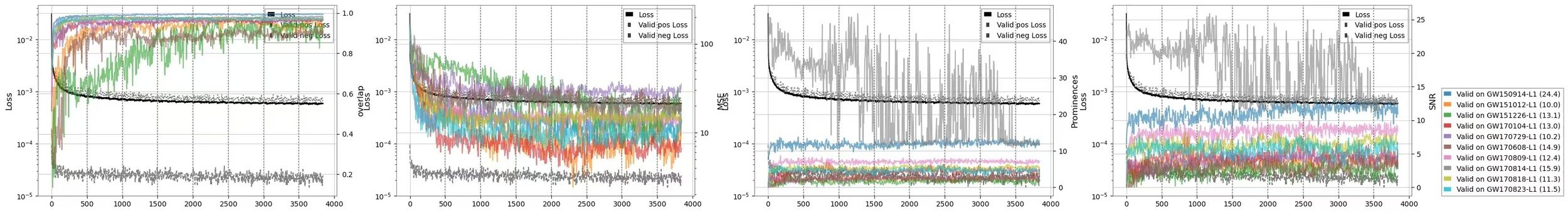
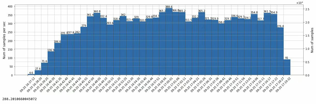
Timestamp distribution of instances in the "memory pool"
Epoch-wise loss & BBH test overlap
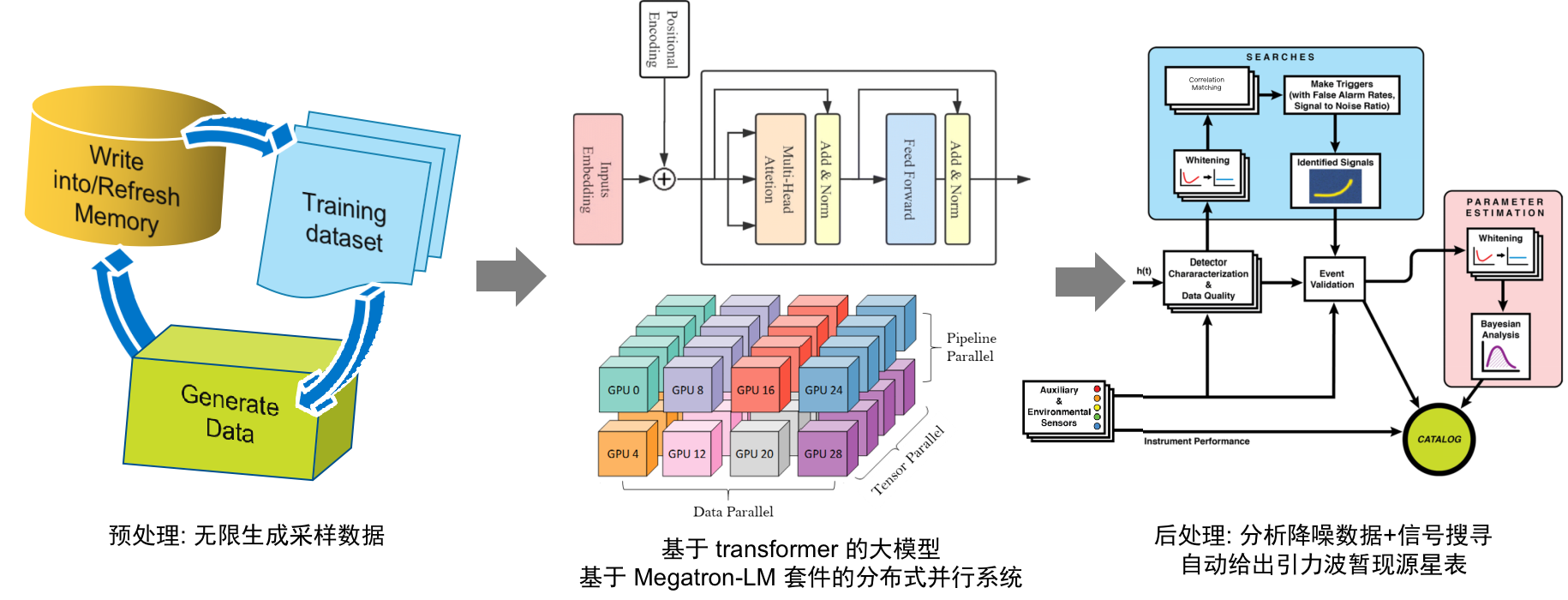
Given sampled signal/noise, randomize peak location and SNR
Continuously append/overwrite signal–noise instances in a fixed-size memory pool, while another process samples randomly for training
Main memory
CPU
DataLoader
GPU memory
GPU
GenTemplate
GenNoise
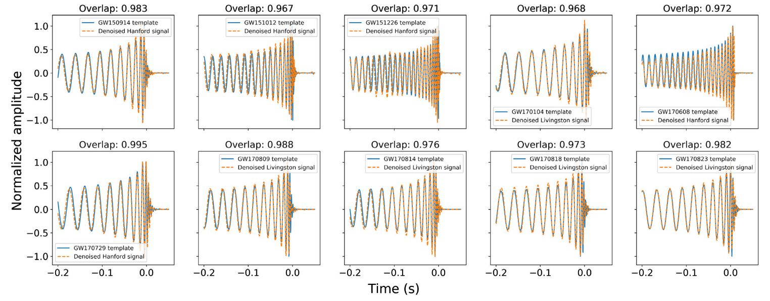
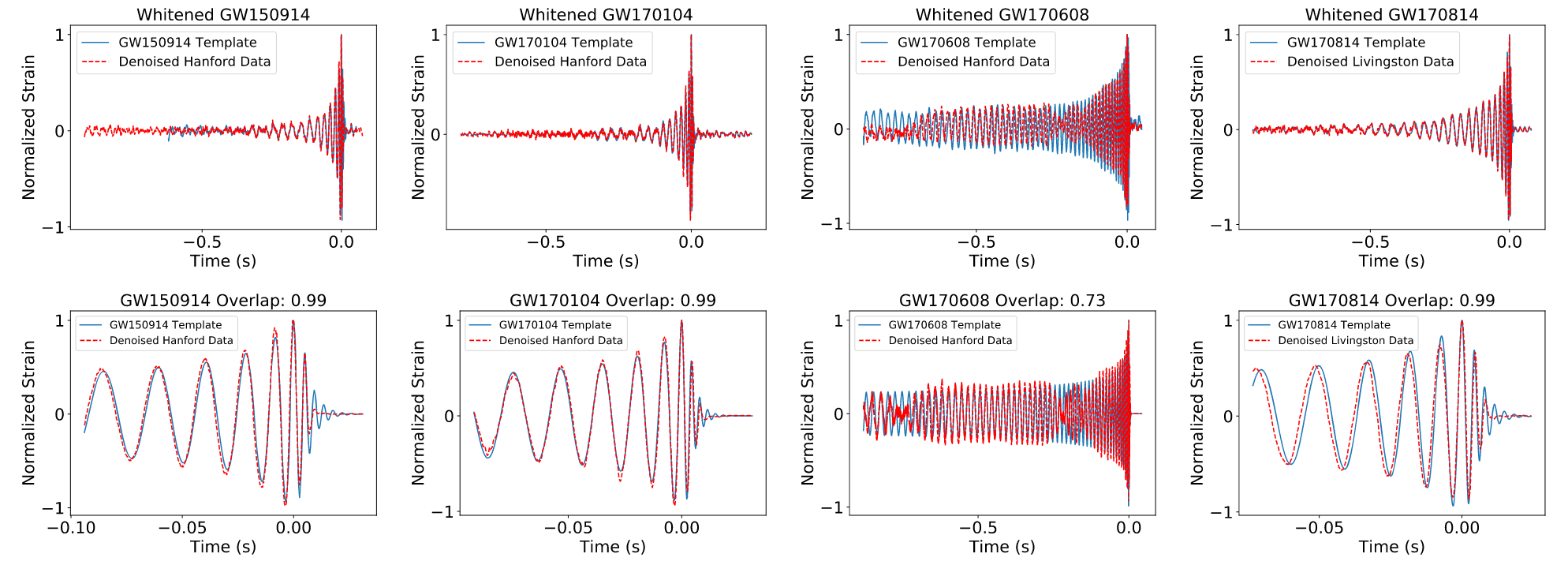
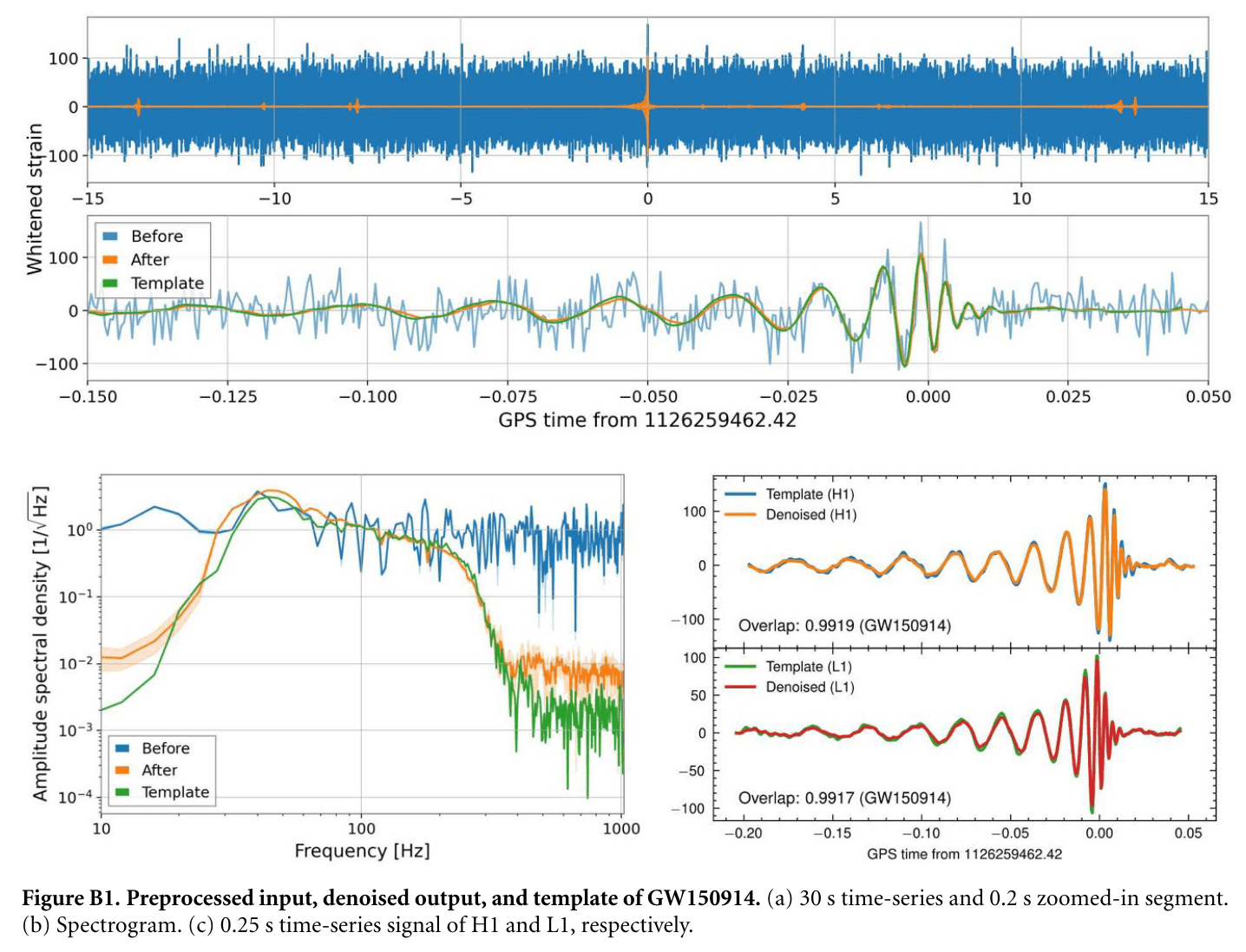
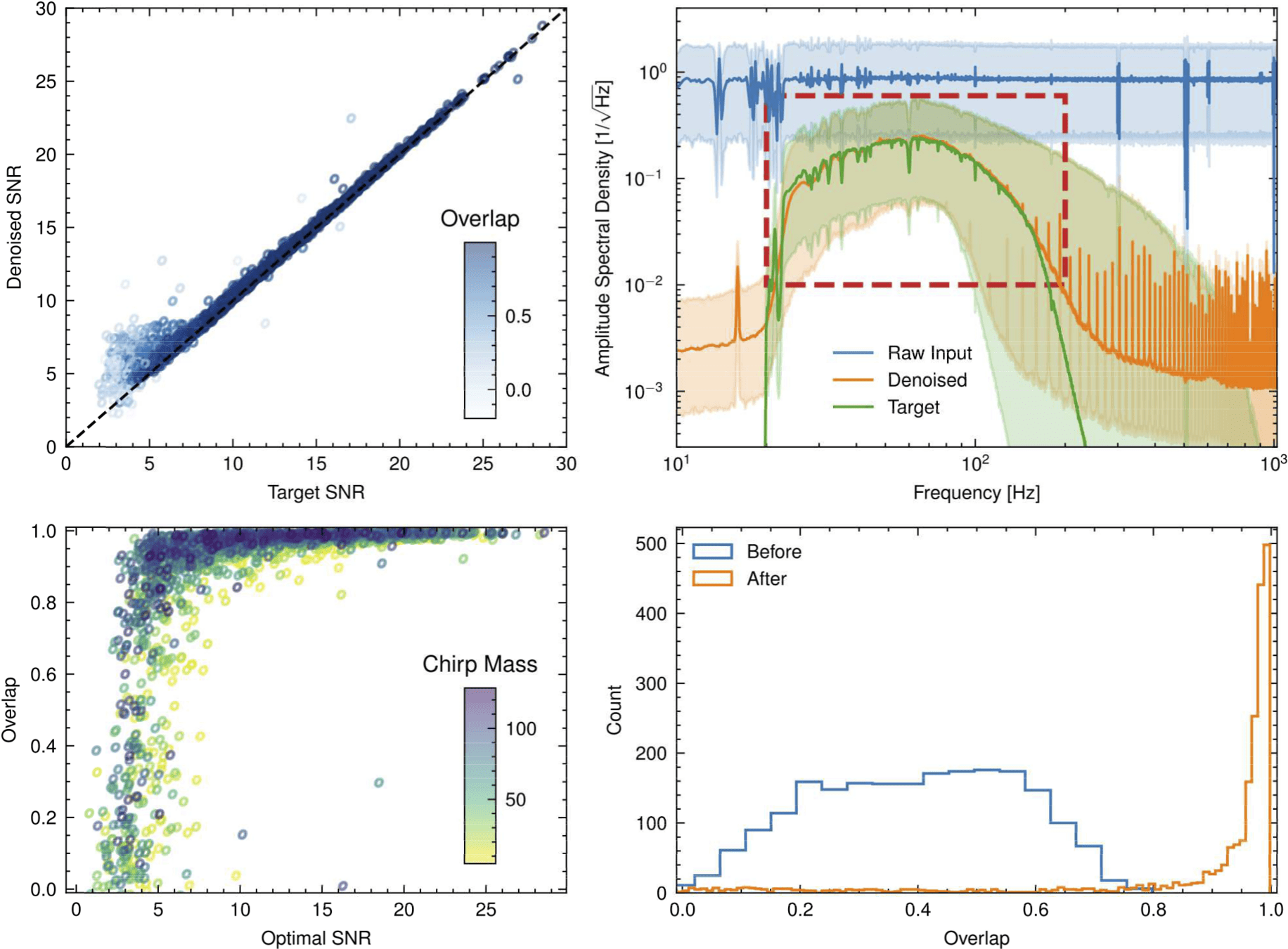
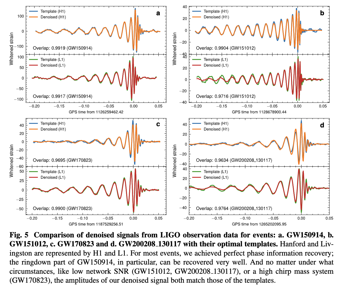
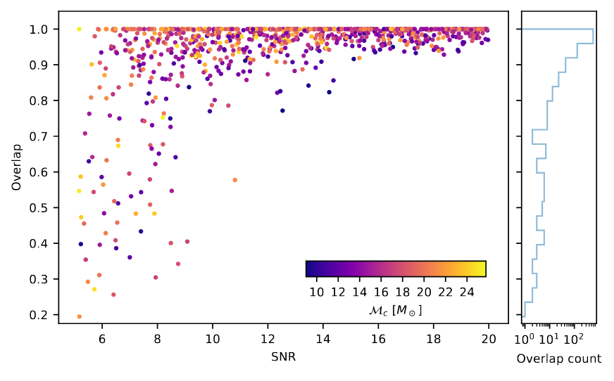
Recovery of Binary Black Holes
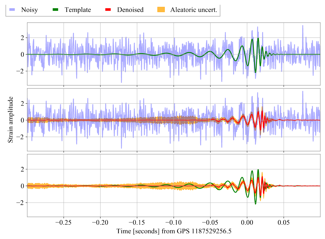
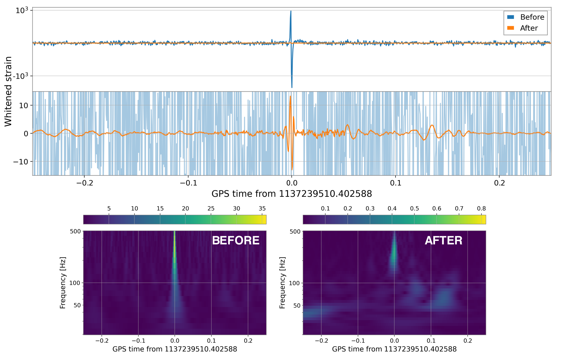
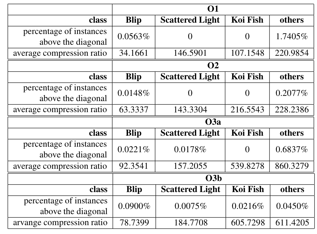
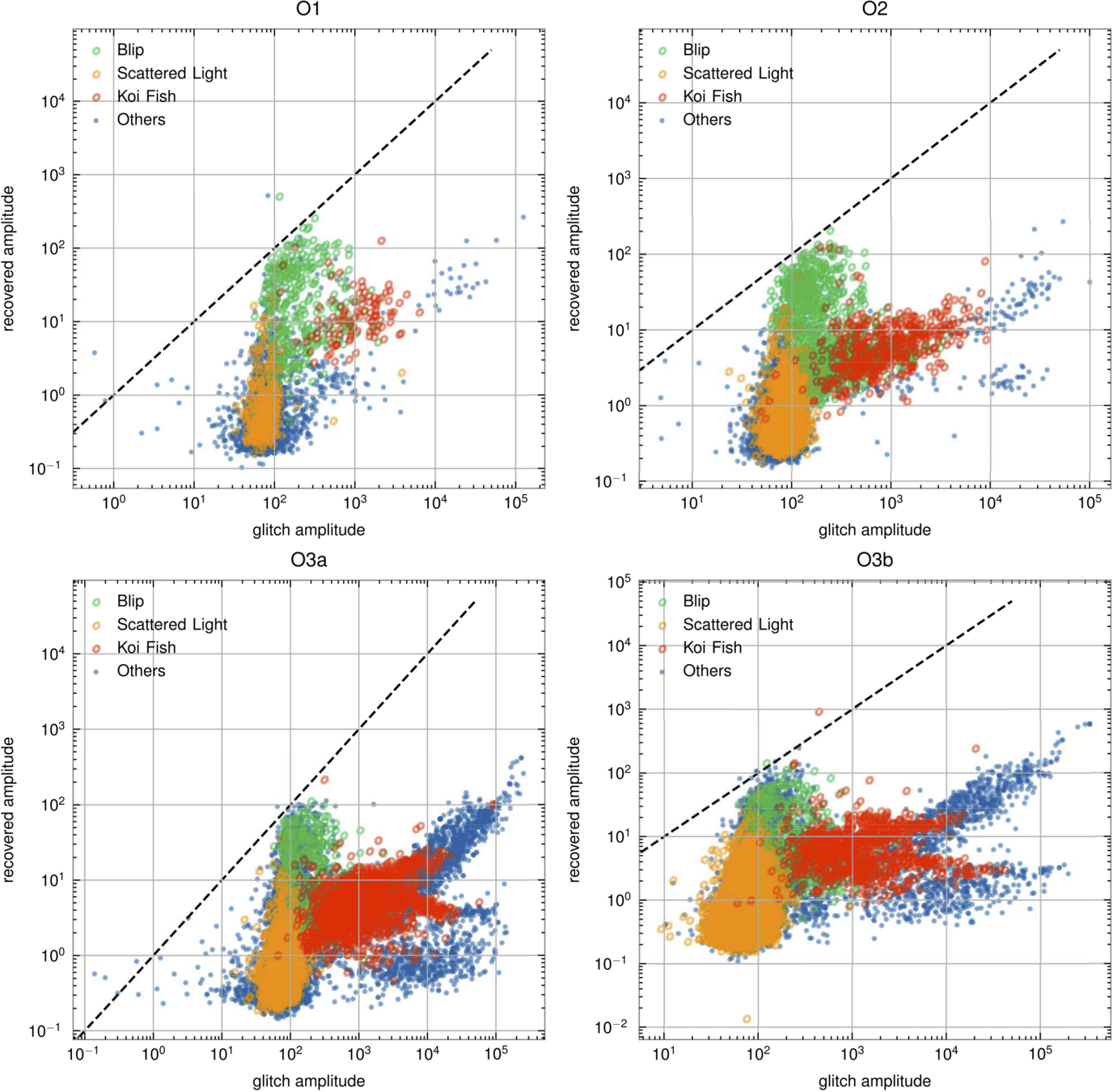
Effect on Realistic Noise (Blip)
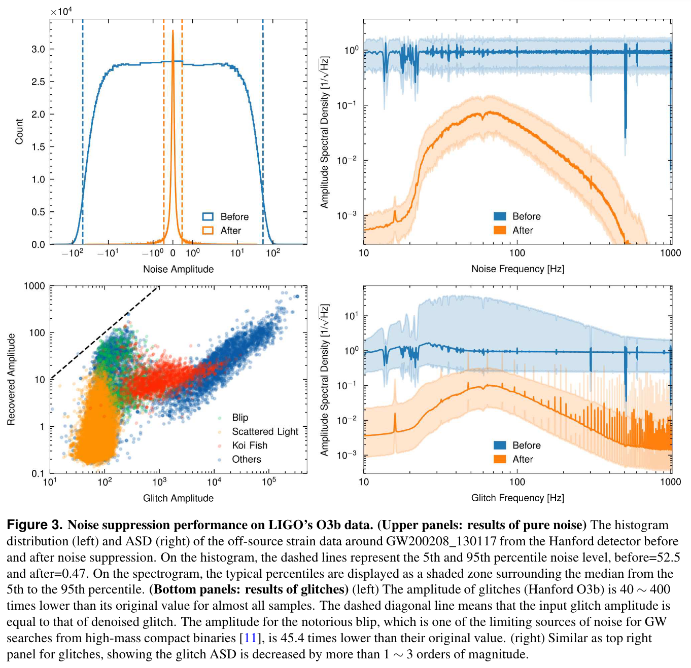
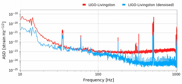
Effect on pure noise
Effect on glitches
Waveformer (OURs)
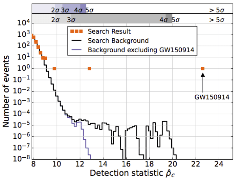
LVK. PRD (2016). arXiv:1602.03839
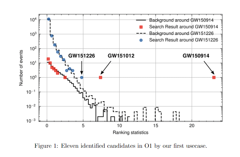
GW151226
GW151012
GW151226
GW151012
LVK. arXiv:1602.03839
He Wang, et al. MLST. 5, 1 (2024): 015046.
A Python Toolbox for Gravitational Wave Astronomy: GWToolkit
Can AI identify new GW events from LIGO data?
Mitigating bias in AI-Driven GW data analysis
Alfaidi & Messerger. arXiv:2402.04589
Menéndez-Vázquez A, et al. PRD 2021
"Draft in Progress"
for _ in range(num_of_audiences):
    print('Thank you for your attention! 🙏')
Slide: DCC-G2502678
Waveformer (OURs)
LVK. PRD (2016). arXiv:1602.03839
GW151226
GW151012
(Bottom panels: results of glitches)
(Upper panels: results of pure noise)
Time-series and spectrogram example of blip.
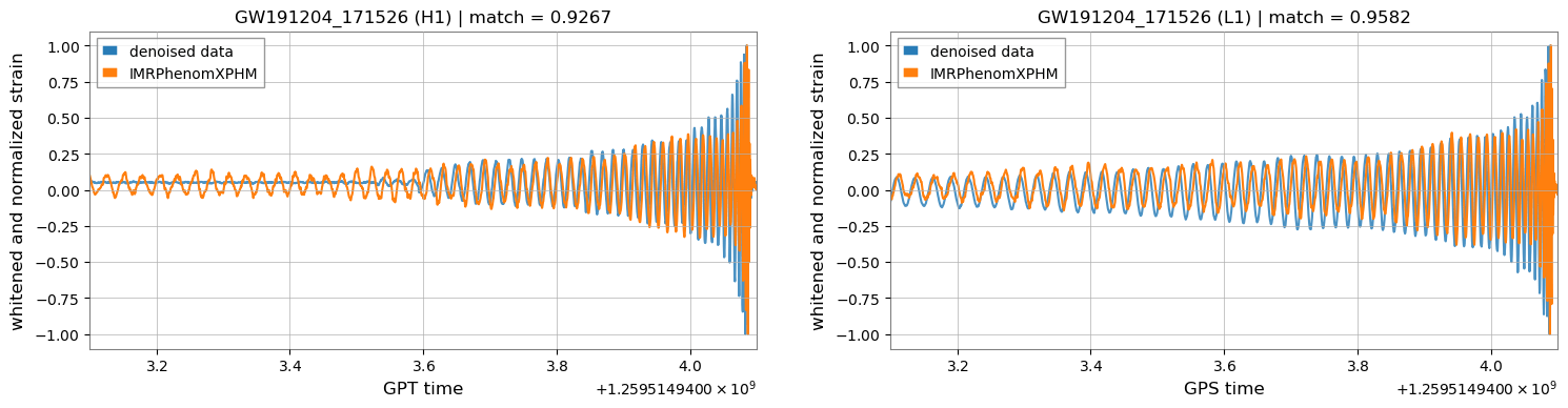
(Upper panels: Signal amplitude recovery performance
(Bottom panels: Signal phase recovery performance)
Bacon P. et al. arXiv: 2205.13513
GW191204_171526
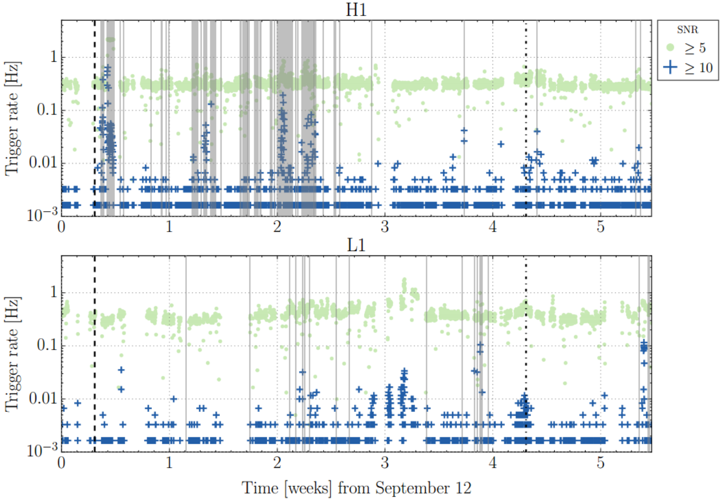
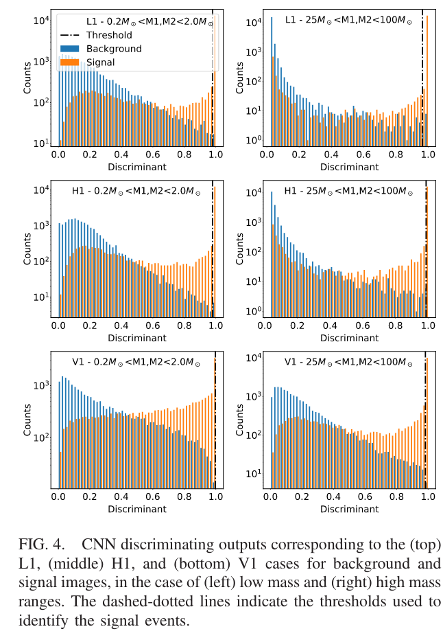
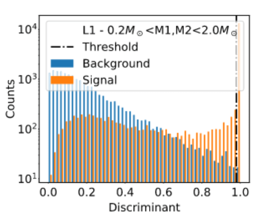
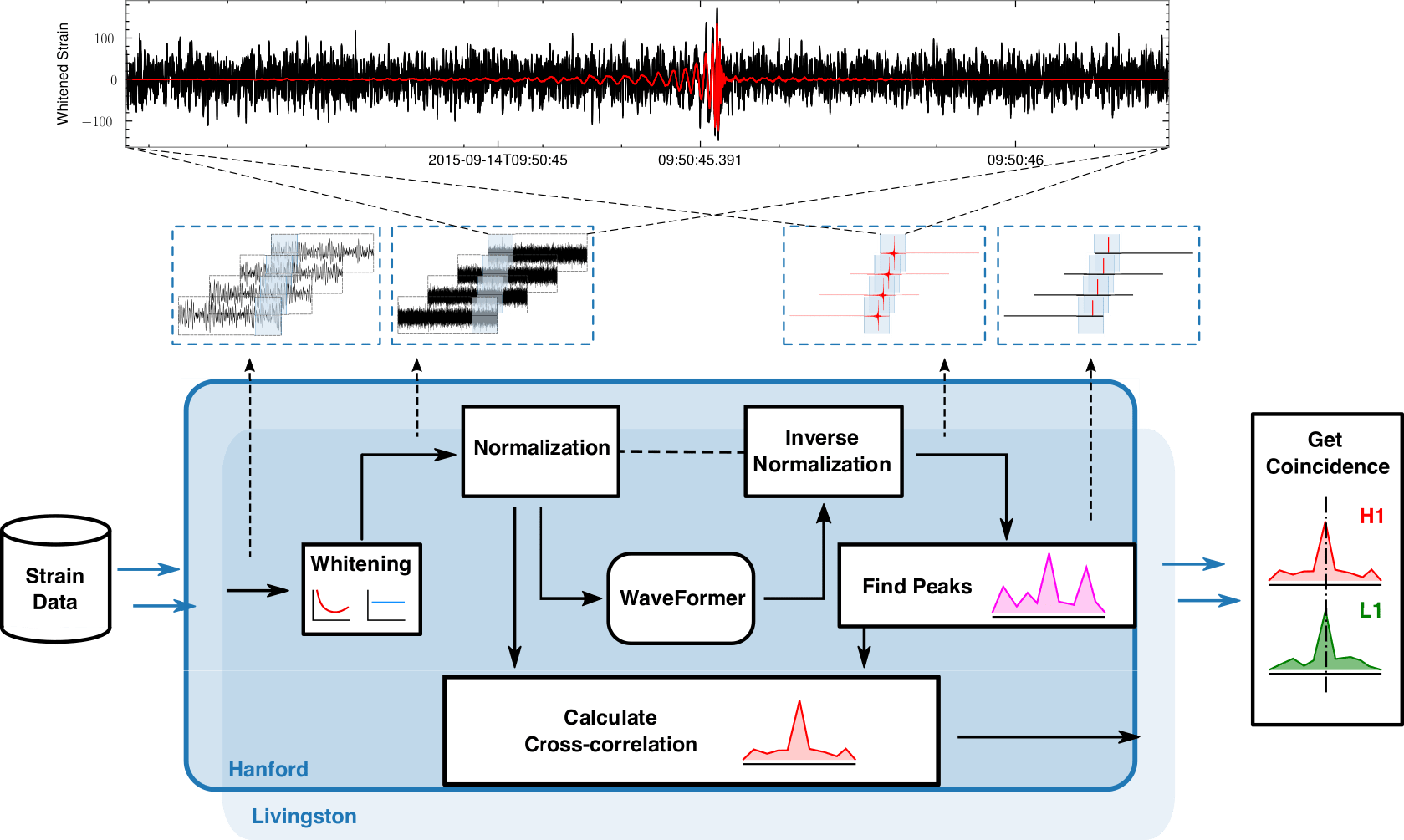
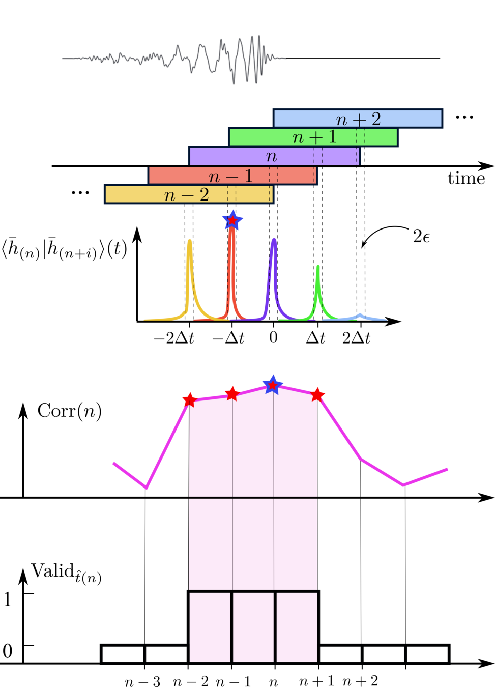
Firstly, we obtain the denoised output by utilizing Waveformer. Then, triggers are defined and identified by three steps including,
Find Peaks. Locate triggers on a single detector by finding its maximum all local-maximum (0.2s away from neighboring maximum/local-maximum).
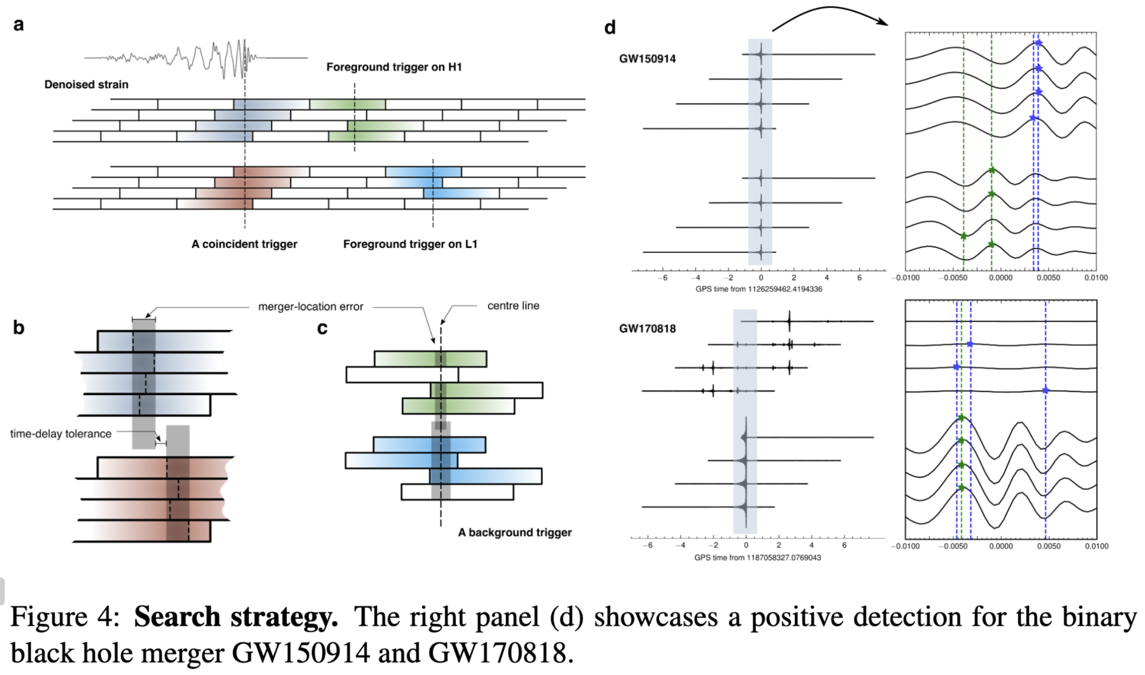
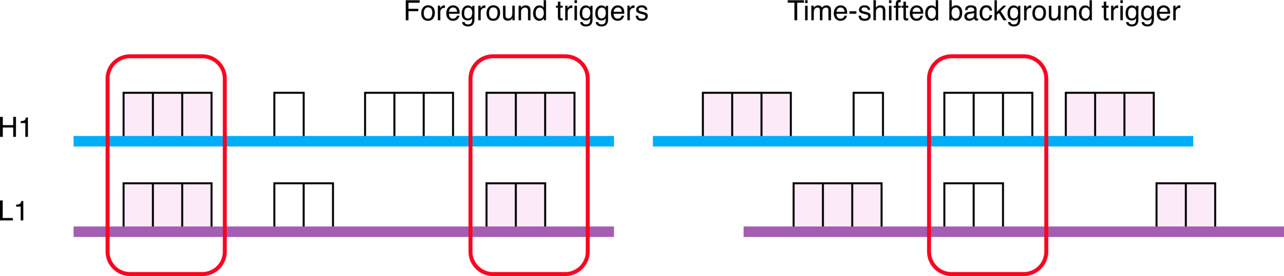
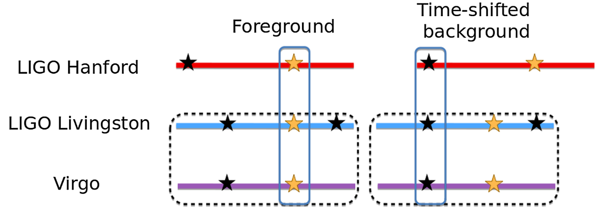
An search algorithm for GW require that: [cite: 2010.07244]
the same signal is seen in the detectors; (the same signal is seen by time-shifting in single detector)
the same waveform must be present both detectors;
and the signal’s time of arrival must be consistent with the GW travel time between the observatories.
Firstly, we obtain the denoised output by utilizing Waveformer. Then, triggers are defined and identified by three steps including,
Find Peaks. Locate triggers on a single detector by finding its maximum all local-maximum (0.2s away from neighboring maximum/local-maximum).
By constraining triggers that exist on both two detectors, we get VALID triggers. (consist 3~4 segments)
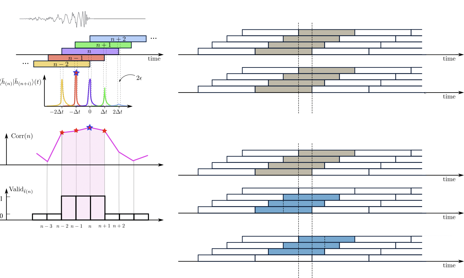
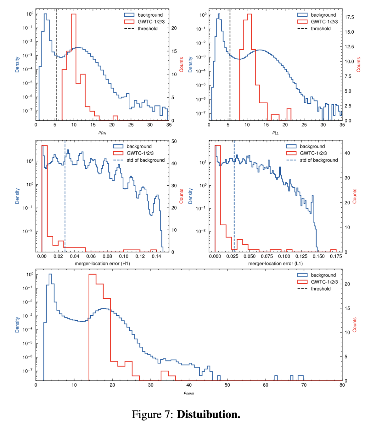
Calculate the correlation of the to-be-evaluated trigger across channels or within a single channel, between its noisy and corresponding denoised segments, as well as between denoised segments themselves.
noisy input segments
denoised output segments
\(\bar{H}\)
\(\bar{L}\)
\({H}\)
\({L}\)
Firstly, we obtain the denoised output by utilizing Waveformer. Then, triggers are defined and identified by three steps including,
Find Peaks. Locate triggers on a single detector by finding its maximum all local-maximum (0.2s away from neighboring maximum/local-maximum).
By constraining triggers that exist on both two detectors, we get VALID triggers. (consist 3~4 segments)
Calculate the correlation of the to-be-evaluated trigger across channels or within a single channel, between its noisy and corresponding denoised segments, as well as between denoised segments themselves.
Waveformer (OURs)
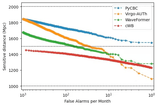
(PyCBC) Davies, et al. PRD 2020
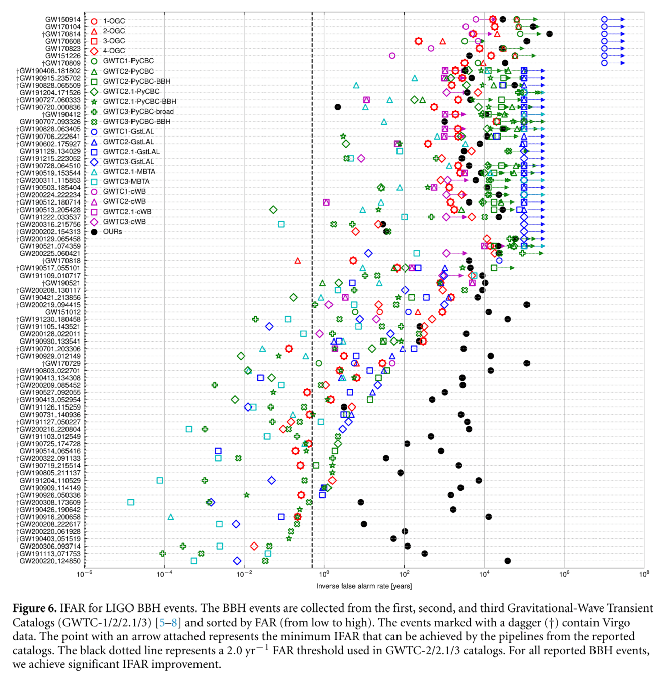
Assessed denoising workflow performance by comparing with GWTC-1, GWTC-2, GWTC2.1, and GWTC-3 catalogs and associated data releases.
Noted significant divergence in IFAR distribution between our results and those from GWTC and OGC catalogs.
Achieved significant IFAR improvement across all 75 reported BBH events, indicating effective suppression of loud terrestrial noise.
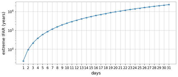
Example: For low SNR (\(10.8_{-0.4}^{+0.3}\)) event GW200208_130117, obtained an IFAR of 8916 years, surpassing maximum IFAR of <4000 years in other catalogs.
Variability in IFAR improvement linked to the original data's noise nature, including its non-Gaussian, non-stationary characteristics, and different signal recognition strategies by pipelines.
IFAR performance significantly depends on the reduction of non-Gaussian noise near each event.
Events with substantial IFAR improvement had misleading non-Gaussian noise effectively eliminated.
Events where IFAR underperforms retained non-Gaussian characteristics, possibly due to WaveFormer's inherent systematic errors.
Evaluating the current workflow as a GW detection demo pipeline on MLGWSC-1 (ds4)
By He Wang
MLA Call (2025/12/18)


