A Tensor Playground:
a demonstration of \(\textsf{TensorSpace}\)
Joshua Maglione
jmaglione@math.uni-bielefeld.de
Universität Bielefeld

Began in 2015 and is still evolving.
Joint with Pete Brooksbank and James Wilson.
Funded in part by NSF: DMS-1620454.
\(\textsf{TensorSpace}\) refers to a collection of Magma packages:
- TensorSpace: data structures for tensors,
- Sylver: algorithms for simultaneous Sylvester equations,
- Densor: algorithms to construct linear closures of tensor spaces.
Constructing Tensors in \(\textsf{TensorSpace}\)
Flexible data structure for tensors
Goal: Want flexible definition for tensors.
Questions: Is a tensor more than just...
- a high-dimensional grid?
- a multilinear map?
How do the questions we want to answer motivate a data structure?
Examples require context
1. \(b\) bilinear form of \(V\). Interpret:
\(\langle b | : V \times V \rightarrowtail K\)
3. \(V\) an \(A\)-module. Interpret:
\(\langle \mu | : V \times A \rightarrowtail V\)
2. \(\psi\) an entangled system of qubits. Interpret:
\(\langle \psi | : \mathbb{C}^2\times \cdots \times \mathbb{C}^2 \rightarrowtail \mathbb{C}\)
Tensors in \(\textsf{TensorSpace}\) are framed
We require tensors to have three things:
1. frame: \((U_0, \ldots, U_n)\),
2. function: \(U_n\times \cdots \times U_1\rightarrowtail U_0\),
3. category*.
*We do not specify now, but we will come back to this.
A "default" category is assigned when not given.
Constructing a tensor from scratch
We construct the tensor
$$\begin{aligned} t : \text{M}_2(\mathbb{Q}) \times \text{M}_2(\mathbb{Q}) &\rightarrowtail \text{M}_2(\mathbb{Q}),\\ (A, B) &\mapsto AB \end{aligned}$$
We have two structures we define:
- frame: \((\text{M}_2(\mathbb{Q}),\; \text{M}_2(\mathbb{Q}),\; \text{M}_2(\mathbb{Q}))\),
- function: \((A, B)\mapsto AB\).
Q := Rationals();
A := MatrixAlgebra(Q, 2);              // 2 x 2 matrices over Q
frame := [A, A, A];
frame;
[
Full Matrix Algebra of degree 2 over Rational Field,
Full Matrix Algebra of degree 2 over Rational Field,
Full Matrix Algebra of degree 2 over Rational Field
]First we define our frame.
Require a function to map a tuple of matrices to their product.
mult := func< x | x[1]*x[2] >;         // <A, B> |-> A*B
t := Tensor(frame, mult);
t;
Tensor of valence 3, U2 x U1 >-> U0
U2 : Full Vector space of degree 4 over Rational Field
U1 : Full Vector space of degree 4 over Rational Field
U0 : Full Vector space of degree 4 over Rational FieldTensors as multilinear functions
Let's do a brief sanity check, and verify \(t\) does what we expect.
X := A![2, 2/5, 0, -1];               // define matrices
Y := A![0, -3, 5, 7];                 // from sequences
X, Y;
[ 2 2/5]
[ 0 -1]
[ 0 -3]
[ 5 7]X*Y, <X, Y> @ t;[ 2 -16/5]
[ -5 -7]
( 2 -16/5 -5 -7)
Recall, the print statement for \(t\): no matrix algebras
t;Tensor of valence 3, U2 x U1 >-> U0
U2 : Full Vector space of degree 4 over Rational Field
U1 : Full Vector space of degree 4 over Rational Field
U0 : Full Vector space of degree 4 over Rational Field
It states vector spaces, but we gave it matrices: \(X\) and \(Y\).
The frame gives context, so that we leave the typing to the machines.
<X, [0, -3, 5, 7]> @ t;
<0, [1, 1, 1, 1]> @ t;
( 2 -16/5 -5 -7)
(0 0 0 0)Structure constants
We define a tensor of the form
$$ \langle t| : K^{d_n} \times \cdots \times K^{d_1} \rightarrowtail K^{d_0} $$
by \(d_0\cdots d_n\) elements in \(K\): a \((d_n\times \cdots \times d_0)\)-grid
$$ [t_{i_n\cdots i_1}^{i_0}]. $$
Notational challenge to do this for general \(n\). We do \(n=2\):
$$ (u, v)\mapsto \left( \sum_{i=1}^{d_2}\sum_{j=1}^{d_1} u_{i}t_{ij}^{1} v_{j}, \ldots, \sum_{i=1}^{d_2}\sum_{j=1}^{d_1} u_{i}t_{ij}^{d_0} v_{j}\right)\in K^{d_0}. $$
Let's construct an example.
d := [3, 2, 5, 4];                 // dimensions of frame
grid := [1..3*2*5*4];              // ints 1, ..., 120
t := Tensor(Q, d, grid);
t;
Tensor of valence 4, U3 x U2 x U1 >-> U0
U3 : Full Vector space of degree 3 over Rational Field
U2 : Full Vector space of degree 2 over Rational Field
U1 : Full Vector space of degree 5 over Rational Field
U0 : Full Vector space of degree 4 over Rational FieldWe verify that the structure constants of \(t\) are what we expect.
StructureConstants(t)[1..10]; // Only first 10 entries[ 1, 2, 3, 4, 5, 6, 7, 8, 9, 10 ]Notice: structure constants are a flat sequence.
The grid model provides easier understanding of data manipulation.
We describe 2 operations that potentially change the frame.
Slicing
Recall, our current tensor has the frame:
$$ \langle t | : \mathbb{Q}^3 \times \mathbb{Q}^2 \times \mathbb{Q}^5 \rightarrow \mathbb{Q}^4 $$
We grab any entry of the grid \([t_{i_n\cdots i_1}^{i_0}]\) and consider the corresponding sub-grid.
This can be interpreted as a tensor itself.
We query for the \(t_{3,2,5}^{4}\) constant:
ind := [{3}, {2}, {5}, {4}];                  // last entry
Slice(t, ind);
[ 120 ]We can query any sequence of indices.
indices := [{1, 3}, {2}, {1, 3, 4}, {4}];     // 2*1*3*1 entries
Slice(t, indices);
[ 24, 32, 36, 104, 112, 116 ]The above example can be interpreted as a new tensor
$$ \langle s | : \mathbb{Q}^2 \times \mathbb{Q} \times \mathbb{Q}^3 \rightarrowtail \mathbb{Q}. $$
So it might be helpful to interpret the output as a matrix.
SliceAsMatrices(t, indices, 3, 1);[
[ 24 32 36]
[104 112 116]
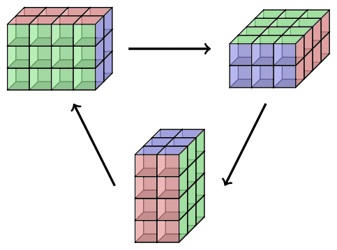
]Shuffling
We apply permutations to the frame. Suppose we are framed by vector spaces
$$ \langle t | : U_n \times \cdots \times U_1\rightarrowtail U_0. $$
For a permutation \(\sigma\) of \(\{0, \ldots, n\}\), a \(\sigma\)-shuffle of \(t\) is a tensor
$$ \langle \sigma(t) | : U_{\sigma(n)} \times \cdots \times U_{\sigma(1)} \rightarrowtail U_{\sigma(0)}. $$
Note: shuffling requires dual-spaces. \(\textsf{TensorSpace}\) handles this.
We continue with current example:
$$ \langle t | : \mathbb{Q}^3 \times \mathbb{Q}^2 \times \mathbb{Q}^5 \rightarrowtail \mathbb{Q}^4. $$
We apply the permutation \(\sigma = (0, 2, 3, 1)\).
sigma := [2, 0, 3, 1];                // cycle: (0, 2, 3, 1)
s := Shuffle(t, sigma);
s;
Tensor of valence 4, U3 x U2 x U1 >-> U0
U3 : Full Vector space of degree 5 over Rational Field
U2 : Full Vector space of degree 3 over Rational Field
U1 : Full Vector space of degree 4 over Rational Field
U0 : Full Vector space of degree 2 over Rational FieldWe can take a look at the structure constants.
StructureConstants(s)[1..10]; // first 10 entries[ 1, 3, 5, 7, 25, 27, 29, 31, 49, 51 ]Recall: the structure constants were \([1, \ldots, 120]\).
Algebras associated to tensors
These definitions work in greater generality, but fix a \(K\)-bilinear map
$$ \langle t | : U\times V\rightarrowtail W. $$
Set \(\Omega = \text{End}(U)\times \text{End}(V)\times \text{End}(W)\). Our algebras are subsets of \(\Omega\).
The first algebra we define is the centroid, and the second is the derivation algebra.
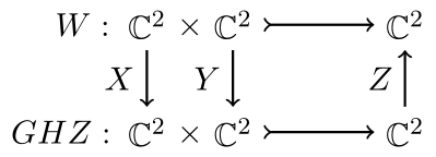
$$ \begin{aligned} \mathcal{C}_t &= \{ (X, Y, Z) \in\Omega \mid \forall u, v,\; \langle t | Xu, v\rangle = \langle t | u, Yv\rangle = Z\langle t | u, v\rangle \} \\ \mathcal{D}_t &= \{ (X, Y, Z) \in \Omega \mid \forall u, v,\; \langle t | Xu, v\rangle + \langle t | u, Yv\rangle = Z\langle t | u, v\rangle \} \end{aligned} $$
Fact. \(\mathcal{C}_t\) is a \(K\)-algebra with \(1\), and \(\mathcal{D}_t\) is a Lie algebra.
Example from quantum info. theory
The GHZ and W states
The Greenberger-Horne-Zeilinger (GHZ) state is
$$ \begin{aligned} \sqrt{2} \cdot GHZ &= |000\rangle + |111\rangle \\ &\equiv (e_1\otimes e_1\otimes e_1) + (e_2\otimes e_2\otimes e_2) \\ &\equiv \begin{bmatrix} (1,0) & (0,0) \\ (0,0) & (0,1) \end{bmatrix}. \end{aligned} $$
The W state is
$$ \begin{aligned} \sqrt{3} \cdot W &= |001\rangle + |010\rangle + |100\rangle \\ &\equiv (e_1\otimes e_1\otimes e_2) + (e_1\otimes e_2\otimes e_1) + (e_2\otimes e_1\otimes e_1) \\ &\equiv \begin{bmatrix} (0,1) & (1,0) \\ (1,0) & (0,0) \end{bmatrix}. \end{aligned} $$
Both states are \((2\times 2\times 2)\)-grids. We interpret these states as
$$ \begin{aligned} \langle GHZ| &: \mathbb{C}^2\times \mathbb{C}^2 \rightarrowtail \mathbb{C}^2 , \\ \langle W| &: \mathbb{C}^2\times \mathbb{C}^2 \rightarrowtail \mathbb{C}^2 \end{aligned} $$
(Typically interpreted as \(\mathbb{C}^2 \times \mathbb{C}^2 \times \mathbb{C}^2 \rightarrowtail \mathbb{C}\).)
Question: \(GHZ\) and \(W\) are contained in the same space. Maybe there is a change of basis (of each \(\mathbb{C}^2\)) that makes GHZ and W equivalent?
(There isn't!)
Let's construct the tensors (over \(\mathbb{Q}\)).
Q := Rationals();
d := [2, 2, 2];                                 // dimensions of frame
GHZ := Tensor(Q, d, [1, 0, 0, 0, 0, 0, 0, 1]);
W := Tensor(Q, d, [0, 1, 1, 0, 1, 0, 0, 0]);
Quick sanity check.
AsMatrices(GHZ, 2, 1);[
[1 0]
[0 0],
[0 0]
[0 1]
]Now we compute their centroids.
C_GHZ := Centroid(GHZ);
C_W := Centroid(W);
C_GHZ, C_W;
Matrix Algebra of degree 6 with 2 generators over Rational Field
Matrix Algebra of degree 6 with 2 generators over Rational Field[
[1 0 0 0 0 0]
[0 1 0 0 0 0]
[0 0 1 0 0 0]
[0 0 0 1 0 0]
[0 0 0 0 1 0]
[0 0 0 0 0 1],
[0 1 0 0 0 0]
[0 0 0 0 0 0]
[0 0 0 1 0 0]
[0 0 0 0 0 0]
[0 0 0 0 0 0]
[0 0 0 0 1 0]
]Basis(C_W);Let's play around with \(\mathcal{C}_W\).
M := C_W.1 + C_W.2;                   // an element of the ring
M;
[1 1 0 0 0 0]
[0 1 0 0 0 0]
[0 0 1 1 0 0]
[0 0 0 1 0 0]
[0 0 0 0 1 0]
[0 0 0 0 1 1]We can get the individual blocks.
X := M @ Induce(C_W, 2);                     // build map
Y := M @ Induce(C_W, 1);                     // for each
Z := M @ Induce(C_W, 0);                     // coordinate
Z;
[1 0]
[1 1]
Verify the centroid satisfies the two equations:
$$ \langle W | Xu, v \rangle = \langle W | u, Yv \rangle = Z \langle W | u, v \rangle. $$
Build two vectors from our \(2\)-dimensional vector space
V := VectorSpace(Q, 2);
u := V![-1, 22/7];
v := V![1/2, 4/27];
u, v;
( -1 22/7)
( 1/2 4/27)<u*X, v> @ W eq <u, v*Y> @ W; // 1st eqn
<u, v*Y> @ W eq (<u, v> @ W)*Z; // 2nd eqntrue
trueWe distinguish \(W\) and \(GHZ\) by the nilpotent elements of their centroids.
J_GHZ := JacobsonRadical(C_GHZ);
J_W := JacobsonRadical(C_W);
Dimension(J_GHZ), Dimension(J_W);
Because the dimension of \(J(GHZ)\) is different from \(J(W)\) these states are inequivalent.
With a little work, one shows that
$$ \begin{aligned} \mathcal{C}_{GHZ} &\cong \mathbb{C}^2, & \mathcal{C}_{W} &\cong \mathbb{C}[x]/\left(x^2\right). \end{aligned} $$
0 1Oh, and just by wiggling your pinky...
The derivation algebras bring their differences to the surface.
D_GHZ := DerivationAlgebra(GHZ);
D_W := DerivationAlgebra(W);
Dimension(D_GHZ), Dimension(D_W);
$$ \dim_{\mathbb{C}}(\mathcal{D}_{GHZ}) = 4 \ne 5 = \dim_{\mathbb{C}}(\mathcal{D}_{W}). $$
4 5Because the dimensions of the derivation algebras are different, \(GHZ\) and \(W\) states are inequivalent.
What is really happening?
The equation \(\langle t | Xu, v\rangle = \langle t | u, Yv\rangle\) becomes
$$ XT^{(k)}_{**} - T^{(k)}_{**}Y = 0, $$where \(T^{(k)}_{**}\) is the \(k\)th slice in the \(0\)-coordinate as a matrix:
$$ T_{**}^{(k)} = \begin{bmatrix} t_{11}^{k} & t_{12}^{k} & \cdots \\ t_{21}^{k} & t_{22}^{k} & \cdots \\ \vdots & \vdots & \ddots \end{bmatrix} $$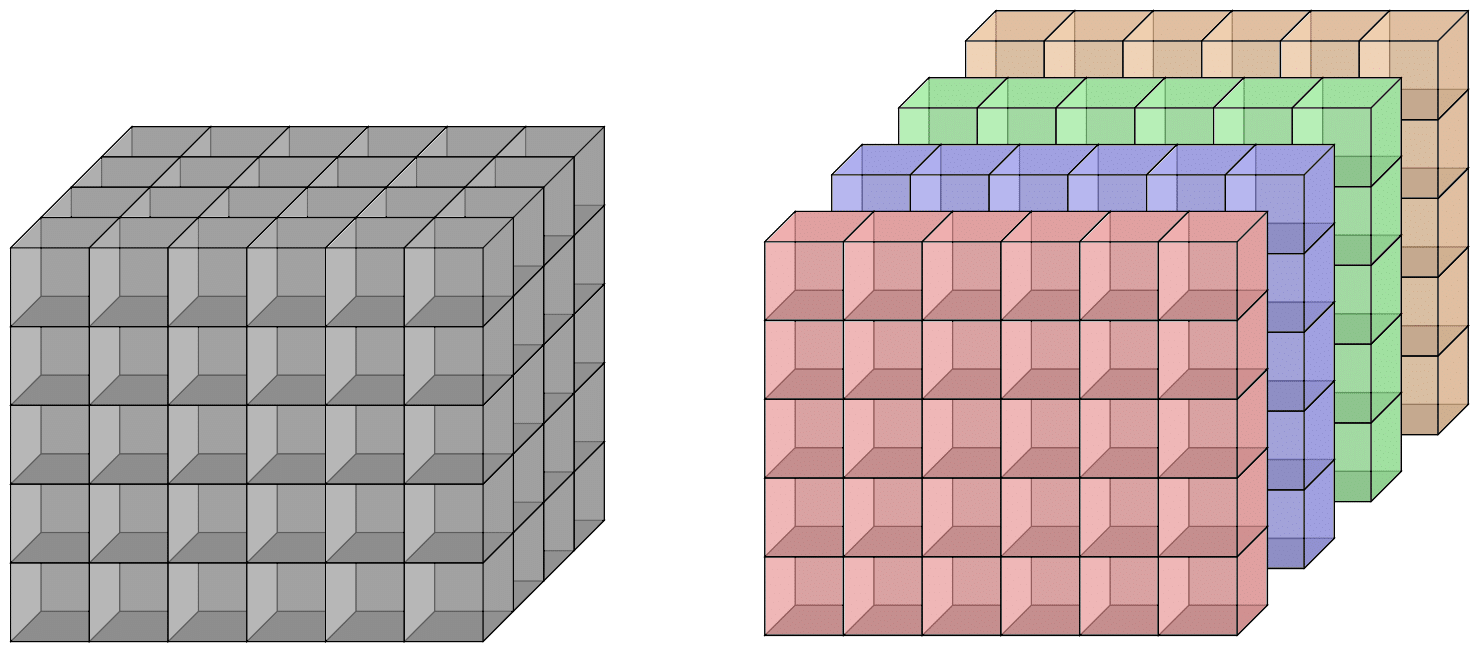
The equation \(\langle t | Xu, v\rangle = Z\langle t | u, v\rangle\) becomes
$$ XT^{*}_{*j} - T^{*}_{*j}Z = 0, $$where \(T^{*}_{*j}\) is the \(j\)th slice in the \(1\)-coordinate as a matrix:
$$ T_{*j}^{*} = \begin{bmatrix} t_{1j}^{1} & t_{1j}^{2} & \cdots \\ t_{2j}^{1} & t_{2j}^{2} & \cdots \\ \vdots & \vdots & \ddots \end{bmatrix} $$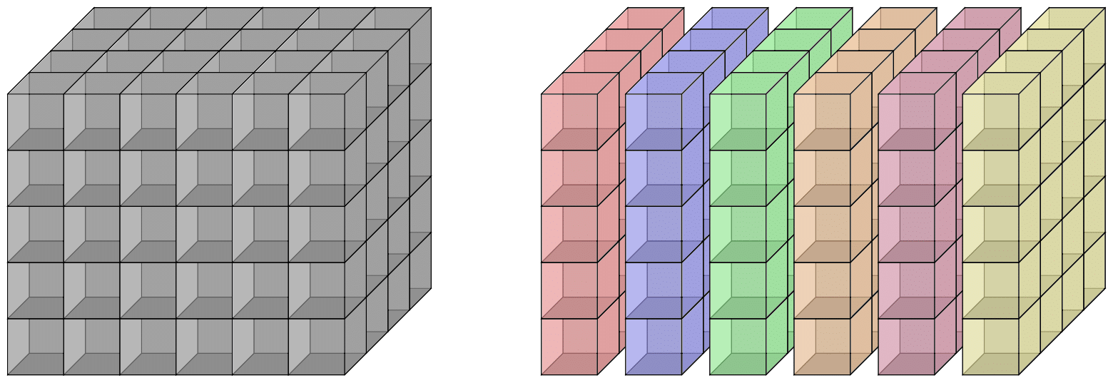
Solving simultaneous Sylvester systems: \(\textsf{Sylver}\)
These algorithms are part of a general family of Sylvester-like equations:
$$ XA + BY = C. $$We need to solve a simultaneous system of Sylvester-like equations.
Naively, this requires \(O(d^7)\) field operations for a \((d\times d\times d)\)-grid.
In general, construct a basis of the kernel of a
\((d_0\cdots d_n) \times (d_0^2 +\cdots + d_n^2)\)-matrix.
Theorem (M.-Wilson 2018).
There is an algorithm to solve simultaneous Sylvester equations of a nondegenerate \((d\times d\times d)\)-grid using \(O(d^4)\) field operations.
Open: Extend this to general tensors and implement.
Tensor spaces & tensor categories
Tensor spaces are the spaces containing tensors. Therefore, defined similarly to tensors.
A tensor space \(T\) is a \(K\)-vector space with
1. a frame \((U_0, \ldots, U_n)\),
2. an interpreter map \(\langle \cdot | : T\rightarrow \left( U_n\times \cdots \times U_1\rightarrowtail U_0\right)\),
3. a category,
4. a basis.
The map \(\langle \cdot |\) gives every \(t\in T\) a multilinear map interpretation
$$ \langle t | : U_n\times \cdots \times U_1\rightarrowtail U_0. $$
Examples that hint towards tensor categories
Equivalence up to a change of bases. The states \(GHZ\) and \(W\) are inequivalent.
For all \(X, Y, Z\in \text{GL}_2(\mathbb{C})\), there exists \(u, v\in\mathbb{C}^2\) such that
$$ \begin{aligned} Z\langle GHZ | Xu, Yv\rangle \ne \langle W | u, v \rangle. \end{aligned} $$
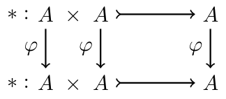
Equivalence of algebras: an isomorphism.
There exists \(\varphi\in\text{GL}(A)\) such that for all \(a,b\in A\)
$$ \begin{aligned} \varphi(ab) &= \varphi(a)\varphi(b). \end{aligned} $$
Adjoint operators of a bilinear form \(\langle\,,\,\rangle\).
For \(u,v\in V\), and \(A\in \text{GL}(V)\),
$$ \begin{aligned} \langle Au, v \rangle &= \langle u, A^*v\rangle. \end{aligned} $$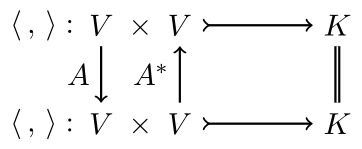
A data structure for tensor categories
For us a tensor category is
1. a function \(\textsf{A}: [n] \rightarrow \{-1, 0, 1\}\),
2. a partition of \([n]\).
The function \(\textsf{A}\) tells us which way the arrows go: \(\downarrow\), \(\parallel\), or \(\uparrow\).
The partition tells us which coordinates are treated as equal.
Examples in \(\textsf{TensorSpace}\)
Let's look at a tensor created earlier: the multiplication in an algebra
$$ \langle t | : \text{M}_2(\mathbb{Q}) \times \text{M}_2(\mathbb{Q}) \rightarrowtail \text{M}_2(\mathbb{Q}). $$
A := MatrixAlgebra(Q, 2);
t := Tensor(A);
TensorCategory(t);
Tensor category of valence 3 (->,->,->) ({ 0, 1, 2 })- all arrows are \(\downarrow\), and
- an operator acts the same way in all three coordinates.
Let's look at an example as a high-dimensional grid.
t := Tensor(GF(2), [2, 3, 2, 3], [1..36]);
t;
Tensor of valence 4, U3 x U2 x U1 >-> U0
U3 : Full Vector space of degree 2 over GF(2)
U2 : Full Vector space of degree 3 over GF(2)
U1 : Full Vector space of degree 2 over GF(2)
U0 : Full Vector space of degree 3 over GF(2)The default tensor category is given.
TensorCategory(t); // default categoryTensor category of valence 4 (->,->,->,->) ({ 1 },{ 2 },{ 0 },{ 3 })Relating tensor spaces & operators
Densor subspaces
The \(GHZ\) and \(W\)-state are not equivalent because derivations were not isomorphic.
For these kinds of questions, we consider spaces of all tensors sharing common operators.
Recall the derivation algebra of \(t\in T\),
$$ \begin{aligned} \mathcal{D}_t &= \{ (X, Y, Z) \in \Omega \mid \forall u, v,\; \langle t | Xu, v\rangle + \langle t | u, Yv\rangle = Z\langle t | u, v\rangle\} \end{aligned} $$
For \(t\in T\), the densor subsapce of \(t\) is the tensor subspace
$$ \textsf{Dens}(t) = \{ s\in T \mid \mathcal{D}_t \subseteq \mathcal{D}_s \}. $$
Example from Lie algebras
Lie algebra of \(3\times 3\) trace zero matrices over a field \(K\), denoted \(\mathfrak{sl}_3\).
The tensor given by the matrix commutator is the following.
K := GF(7);
sl3 := LieAlgebra("A2", K);
t := Tensor(sl3);
t;
Tensor of valence 3, U2 x U1 >-> U0
U2 : Full Vector space of degree 8 over GF(7)
U1 : Full Vector space of degree 8 over GF(7)
U0 : Full Vector space of degree 8 over GF(7)Few tensors contain an \(8\)-dimensional Lie algebra.
Note the tensor category.
TensorCategory(t);Tensor category of valence 3 (->,->,->) ({ 0, 1, 2 })Each operator acts the same on each of the three coordinates.
From standard results, \(\mathcal{D}_t \cong \mathfrak{sl}_3\).
D := DerivationAlgebra(t);
Dimension(D);8The densor subspace of \(t\) is computed using \(\textsf{Densor}\).
Dens := UniversalDensorSubspace(t);
Dens;
Tensor space of dimension 2 over GF(7) with valence 3
U2 : Full Vector space of degree 8 over GF(7)
U1 : Full Vector space of degree 8 over GF(7)
U0 : Full Vector space of degree 8 over GF(7)The dimension of the densor subspace is tiny compared to the ambient space.
T := Parent(t);                      // full tensor space of t
Dimension(T), Dimension(Dens);
512 2What just happened?
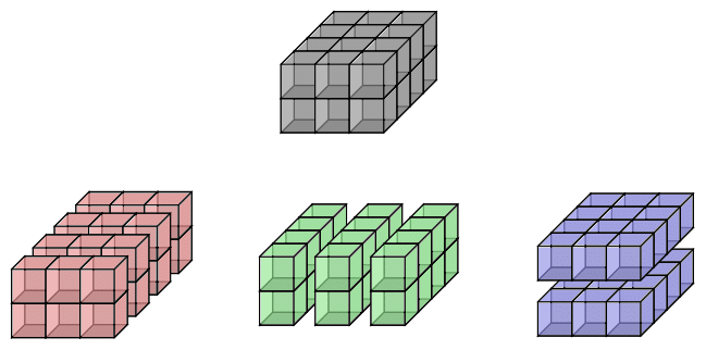
Example: matrix multiplication
The tensor space \(T\) framed by \((K^{12}, K^8, K^6)\) contains
$$ \langle t | : \text{M}_{3\times 4} \times \text{M}_{4\times 2} \rightarrowtail \text{M}_{3\times 2}. $$t := MatrixTensor(Q, [3, 4, 2]);
t;Tensor of valence 3, U2 x U1 >-> U0
U2 : Full Vector space of degree 12 over Rational Field
U1 : Full Vector space of degree 8 over Rational Field
U0 : Full Vector space of degree 6 over Rational FieldThe derivation algebra of \(t\) is large because matrix multiplication is distributive.
Recall the derivation equation:
$$ \langle t | Xu, v\rangle + \langle t | u, Yv \rangle = Z\langle t | u, v \rangle $$
If \(X\in \text{M}_{3\times 3}\), then we re-interpret
$$ (XU)*V + U*(0V) = X(U*V). $$
Similar equations hold for \(Y\in\text{M}_{4\times 4}\) and \(Z\in\text{M}_{2\times 2}\).
Therefore, \(\text{M}_{3\times 3} \cup \text{M}_{4\times 4} \cup \text{M}_{2\times 2} \subseteq \mathcal{D}_t\).
We denote the algebra \(\text{M}_{n\times n}\) with the matrix commutator by \(\mathfrak{gl}_n\).
Fact. \(\mathcal{D}_t \cong \left(\mathfrak{gl}_3\oplus \mathfrak{gl}_4 \oplus\mathfrak{gl}_2\right)/K\).
D := DerivationAlgebra(t);
Dimension(D) eq (3^2 + 4^2 + 2^2 - 1);           // compare dimensions
We can easily verify that the dimensions match.
trueDens := UniversalDensorSubspace(t);
Dens;Tensor space of dimension 1 over Rational Field with valence 3
U2 : Full Vector space of degree 12 over Rational Field
U1 : Full Vector space of degree 8 over Rational Field
U0 : Full Vector space of degree 6 over Rational FieldWith derivaton algebra so large, the densor subspace must be small.
Therefore, in a \(576\)-dimensional space, \(T\), matrix multiplication is set apart from the rest.
As a consequence, the symmetries of \(t\) are completely determined by its derivations.
How are densor spaces computed?
A dual solve to derivations
Recall, we consider Sylvester-like systems of the form:
$$ XT_{**}^{(k)} + T_{**}^{(k)}Y = 0 $$
The same system is used to get the densor subspace$-$the roles are swapped.
We are given the derivation algebra, so we slice a symbolic tensor.
Simultaneously solve a "dual" version of the Sylvester-like equations.
Theorem. (Brooksbank-M.-Wilson)
There exists an algorithm to simultaneously solve a "dual" Sylvester-like system using \(O(d^9m^2)\) field operations, given \(m\) operators acting on a \((d\times d\times d)\)-grid.
Open: Does a similar improvement apply for these equations as well? What is the resulting complexity?
Summary
- Still uncovering new algebraic data from tensors, and this is a snapshot of \(\textsf{TensorSpace}\).
- Context through the frame and tensor category give flexibility in the data structures.
- These algebras provide general tools to different kinds of applications.
A Tensor Playground: a demonstration of TensorSpace
By Josh Maglione
A Tensor Playground: a demonstration of TensorSpace
New algorithms for tensors change the way we compute with and manipulate tensors. Making room for modern theory while keeping the tried and true is the purpose of TensorSpace. We demonstrate how to build a tensor space system and apply it to known problems.