Bridging Simulators with Conditional Optimal Transport
Justine Zeghal, Benjamin Remy,
Yashar Hezaveh, François Lanusse,
Laurence Perreault-Levasseur






Field Level Meeting SkAI, Chicago
February 2026
\underbrace{p(\theta|x=x_0)}_{\text{posterior}}
\underbrace{p(x = x_0|\theta)}_{\text{likelihood}}
\propto
Full-field inference: extracting all cosmological information
\underbrace{p(\theta)}_{\text{prior}}
Bayes theorem:
\underbrace{p(\theta|x=x_0)}_{\text{posterior}}
\underbrace{p(x = x_0|\theta)}_{\text{likelihood}}
\propto
Full-field inference: extracting all cosmological information
\underbrace{p(\theta)}_{\text{prior}}
Bayes theorem:
\underbrace{p(\theta|x=x_0)}_{\text{posterior}}
\underbrace{p(x = x_0|\theta)}_{\text{likelihood}}
\propto
Full-field inference: extracting all cosmological information
\underbrace{p(\theta)}_{\text{prior}}
Bayes theorem:
\underbrace{p(\theta|x=x_0)}_{\text{posterior}}
\underbrace{p(x = x_0|\theta)}_{\text{likelihood}}
\propto
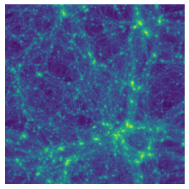
Full-field inference: extracting all cosmological information
\underbrace{p(\theta)}_{\text{prior}}
\theta
Simulator
x
Bayes theorem:
\underbrace{p(\theta|x=x_0)}_{\text{posterior}}
\underbrace{p(x = x_0|\theta)}_{\text{likelihood}}
\propto
Bayes theorem:
Full-field inference: extracting all cosmological information
\underbrace{p(\theta)}_{\text{prior}}
\theta
Simulator
x
Two ways to get the posterior:
- Explicit inference:
\rightarrow \text{we need } \nabla_{\theta, z} \log p(x,\theta, z)
\rightarrow \text{we need } (x, \theta) \sim p(x, \theta, z)
- Implicit inference
\underbrace{p(\theta|x=x_0)}_{\text{posterior}}
\underbrace{p(x = x_0|\theta)}_{\text{likelihood}}
\propto
Full-field inference: extracting all cosmological information
\underbrace{p(\theta)}_{\text{prior}}
\theta
Simulator
x
Two ways to get the posterior:
- Explicit inference:
\rightarrow \text{we need } \nabla_{\theta, z} \log p(x,\theta, z)
\rightarrow \text{we need } (x, \theta) \sim p(x, \theta, z)
- Implicit inference
Has to be realistic!
Bayes theorem:
Wrong models generate bias
Fast simulations
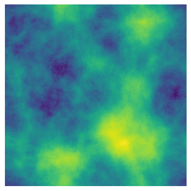
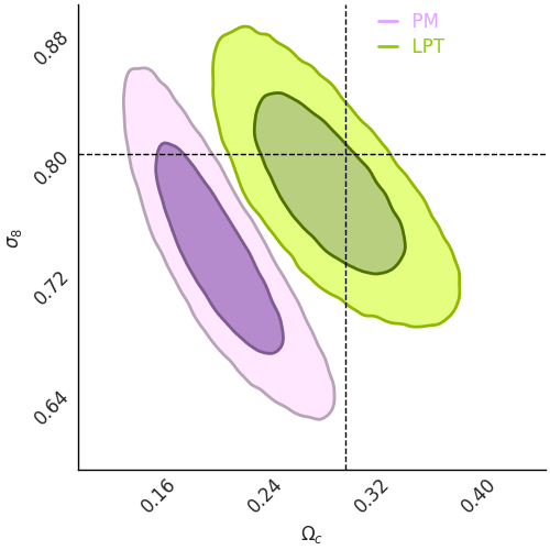
Costly simulations
Wrong models generate bias
→ e.g. full nbody, hydro
\log p(x)
Fast simulations
Costly simulations
| O(ms) runtime | ❌ |
| differentiable | ❌ |
| ❌ | |
| realistic | ✅ |
Wrong models generate bias
→ e.g. full nbody, hydro
\log p(x)
\log p(x)
→ e.g. log-normal, LPT, PM
| O(ms) runtime | ✅ |
| differentiable | ✅ |
| ✅ | |
| realistic | ❌ |
Fast simulations
Costly simulations
| O(ms) runtime | ❌ |
| differentiable | ❌ |
| ❌ | |
| realistic | ✅ |
Learning the correction
We can learn
the correction!
Fast simulations
Costly simulations
Learning the correction
We can learn
the correction!
Fast simulations
x_1 = \phi(x_0)
- it preserves the conditioning,
Costly simulations
\text{We seek a mapping } \phi:
- ,
such that
- it minimally correct the simulation.
x_1 \sim p_1(x \mid \theta)
Learning the correction
We can learn
the correction!
Fast simulations
x_1 = \phi(x_0)
- it preserves the conditioning,
Costly simulations
\text{We seek a mapping } \phi:
- ,
such that
- it minimally correct the simulation.
Requirements:
- has to map to a distribution sample.
\phi
- has to work in high dimensions.
\phi
- has to bridge any two distributions.
\phi
- has to bridge conditional distributions.
\phi
- has to be the solution of the OT problem.
\phi
x_1 \sim p_1(x \mid \theta)
Conditional Optimal Transport Flow Matching
Conditional Optimal Transport Flow Matching
(Lipman et al. 2023)
Flow matching
f^{-1}_1
f^{-1}_2
f_1
f_2
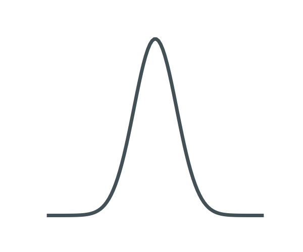
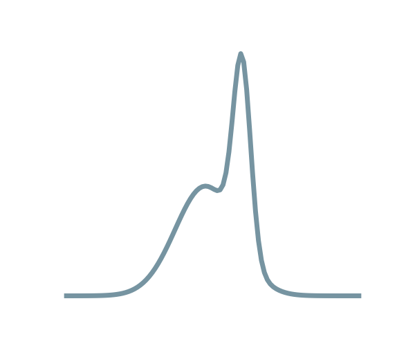
x_0 \sim p_0
x_1 \sim p_1
x_t \sim p_t
x_0 \sim p_0
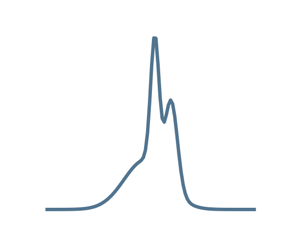
(Lipman et al. 2023)
Flow matching
f^{-1}_1
f^{-1}_2
f_1
f_2
x_0 \sim p_0
x_1 \sim p_1
x_t \sim p_t
x_0 \sim p_0
\rightarrow \text{ learn discrete}\\
\text{ transformations } f_t
(Lipman et al. 2023)
Flow matching
f^{-1}_1
f^{-1}_2
f_1
f_2
x_0 \sim p_0
x_1 \sim p_1
x_t \sim p_t
x_0 \sim p_0
\rightarrow \text{ learn discrete}\\
\text{ transformations } f_t

x_0 \sim p_0
x_1 \sim p_1
x_t \sim p_t
\rightarrow \text{ learn continuous }\\
\text{ transformations } f_t \\
\text{ solution of }\\
\frac{d x_t}{dt} = \color{#ce6eff}{v_\varphi}\color{black}{(x_t, t)}
x_0 \sim p_0
x_0 \sim p_0
x_1 \sim p_1
x_t \sim p_t
x_0 \sim p_0
x_0 \sim p_0
x_1 \sim p_1
x_t \sim p_t
\rightarrow \text{ learn continuous }\\
\text{ transformations } f_t \\
\text{ solution of }\\
\frac{d x_t}{dt} = \color{#ce6eff}{v_\varphi}\color{black}{(x_t, t)}
f^{-1}_1
f^{-1}_2
f_1
f_2
x_0 \sim p_0
x_0 \sim p_0
x_1 \sim p_1
x_t \sim p_t
x_0 \sim p_0
x_0 \sim p_0
x_1 \sim p_1
x_t \sim p_t
x_0 \sim p_0
\rightarrow \text{ learn discrete}\\
\text{ transformations } f_t
\mathcal{L}_{FM}(\theta) = \mathbb{E}_{p(t)q(x_0,x_1)p_t(x_t\mid x_0,x_1)} \Big[ \| \color{#ce6eff}{v_\varphi} \color{black}{(x_t, t)- v(x_t,t) \|^2 \Big]}
(Lipman et al. 2023)
Flow matching
x_0 \sim p_0
x_1 \sim p_1
x_t \sim p_t
\rightarrow \text{ learn continuous }\\
\text{ transformations } f_t \\
\text{ solution of }\\
\frac{d x_t}{dt} = \color{#ce6eff}{v_\varphi}\color{black}{(x_t, t)}
f^{-1}_1
f^{-1}_2
f_1
f_2
x_0 \sim p_0
x_0 \sim p_0
x_1 \sim p_1
x_t \sim p_t
x_0 \sim p_0
x_0 \sim p_0
x_1 \sim p_1
x_t \sim p_t
x_0 \sim p_0
\rightarrow \text{ learn discrete}\\
\text{ transformations } f_t
\mathcal{L}_{FM}(\theta) = \mathbb{E}_{p(t)q(x_0,x_1)p_t(x_t\mid x_0,x_1)} \Big[ \| \color{#ce6eff}{v_\varphi} \color{black}{(x_t, t)- v(x_t,t) \|^2 \Big]}
p(x_t\mid x_0,x_1) = \mathcal{N}((1-t)x_1 + t x_0, \sigma)
(Lipman et al. 2023)
Flow matching
v(x_t, t) = x_1 - x_0
Requirements:
- has to map to a distribution sample.
\phi
- has to work in high dimensions.
\phi
- has to bridge any two distributions.
\phi
- has to bridge conditional distributions.
\phi
- has to be the solution of the OT problem.
\phi
✅
✅
✅
Conditional Optimal Transport Flow Matching
Requirements:
- has to map to a distribution sample.
\phi
- has to work in high dimensions.
\phi
- has to bridge any two distributions.
\phi
- has to bridge conditional distributions.
\phi
- has to be the solution of the OT problem.
\phi
✅
✅
✅
Conditional Optimal Transport Flow Matching
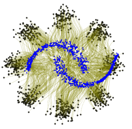
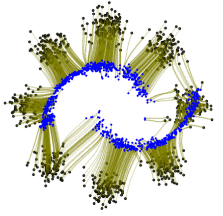
Optimal Transport Flow matching (Tong et al. 2024)
Flow Matching loss function:
\rightarrow (x_0, x_1) \sim p_0(x_0)p_1(x_1)
Indepent coupling:
Optimal Transport coupling:
\rightarrow (x_0, x_1) \sim \pi^*(x_0,x_1)
W(q_0, q_1)^2_2 = \inf_{p_t, v_t} \int_{\mathbb{R}^d}\int^1_0 p_t(x)\|v_t(x)\|^2 dt dx
i.e. minimizes the path for all trajectories between and .
p_0
p_1
\text{ with } \pi^*= \inf_{\pi} \int_{{\mathbb{R}^d}^2} ||x_0 - x_1||^2 d\pi(x_0,x_1)
This coupling, combined with the linear interpolant, solve the dynamic OT:
x_0 \sim p_0
\color{blue}{x_1 \sim p_1}
p(x_t\mid x_0,x_1) = \mathcal{N}((1-t)x_1 + t x_0, \sigma)
\mathcal{L}_{FM}(\theta) = \mathbb{E}_{p(t)q(x_0,x_1)p_t(x_t\mid x_0,x_1)} \Big[ \| \color{#ce6eff}{v_\varphi} \color{black}{(x_t, t)- (x_1-x_0) \|^2 \Big]}
Requirements:
- has to map to a distribution sample.
\phi
- has to work in high dimensions.
\phi
- has to bridge any two distributions.
\phi
- has to bridge conditional distributions.
\phi
- has to be the solution of the OT problem.
\phi
✅
✅
✅
Conditional Optimal Transport Flow Matching
✅
Requirements:
- has to map to a distribution sample.
\phi
- has to work in high dimensions.
\phi
- has to bridge any two distributions.
\phi
- has to bridge conditional distributions.
\phi
- has to be the solution of the OT problem.
\phi
✅
✅
✅
Conditional Optimal Transport Flow Matching
✅
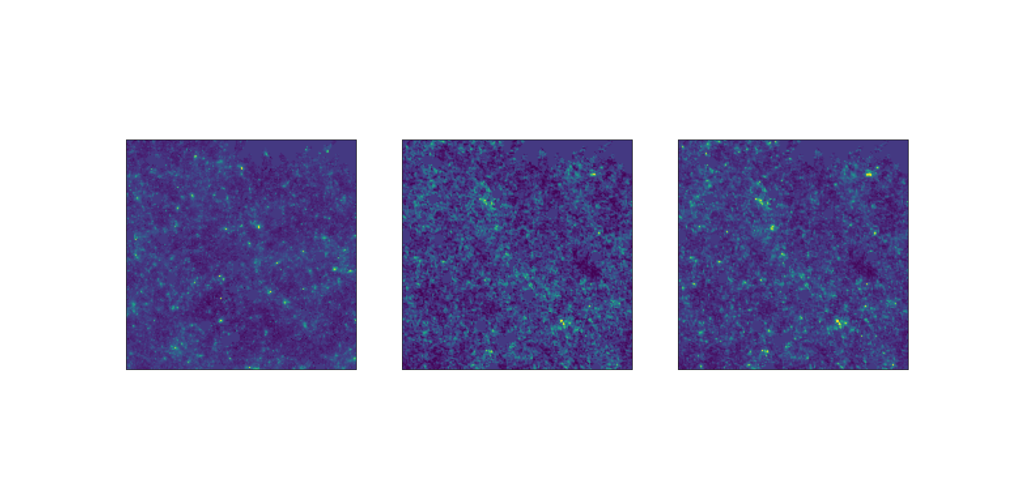
Conditional Optimal Transport Flow matching (Kerrigan et al. 2024)
OT Flow Matching loss function:
\text{ where } \pi^*= \inf_{\pi} \int_{{\mathbb{R}^d}^2} ||x_0 - x_1||^2 d\pi(x_0,x_1)
v_\varphi\left[\begin{matrix} \theta \\ x \end{matrix}\right] = \left[\begin{matrix} v_\varphi(\theta, t) \\ v_\varphi(\theta, x, t) \end{matrix}\right] = \left[\begin{matrix} 0 \\ v_\varphi(\theta, x, t) \end{matrix}\right]
c(x_0,x_1, \theta_0, \theta_1)= \|\theta_1 - \theta_0 \|^2 + \epsilon \|x_1 - x_0 \|^2
p(x_t\mid x_0,x_1) = \mathcal{N}((1-t)x_1 + t x_0, \sigma) \text{ with } (x_0, x_1) \sim \pi^*(x_0,x_1)
\mathcal{L}_{FM}(\theta) = \mathbb{E}_{p(t)q(x_0,x_1)p_t(x_t\mid x_0,x_1)} \Big[ \| \color{#ce6eff}{v_\varphi} \color{black}{(x_t, t)- (x_1-x_0) \|^2 \Big]}
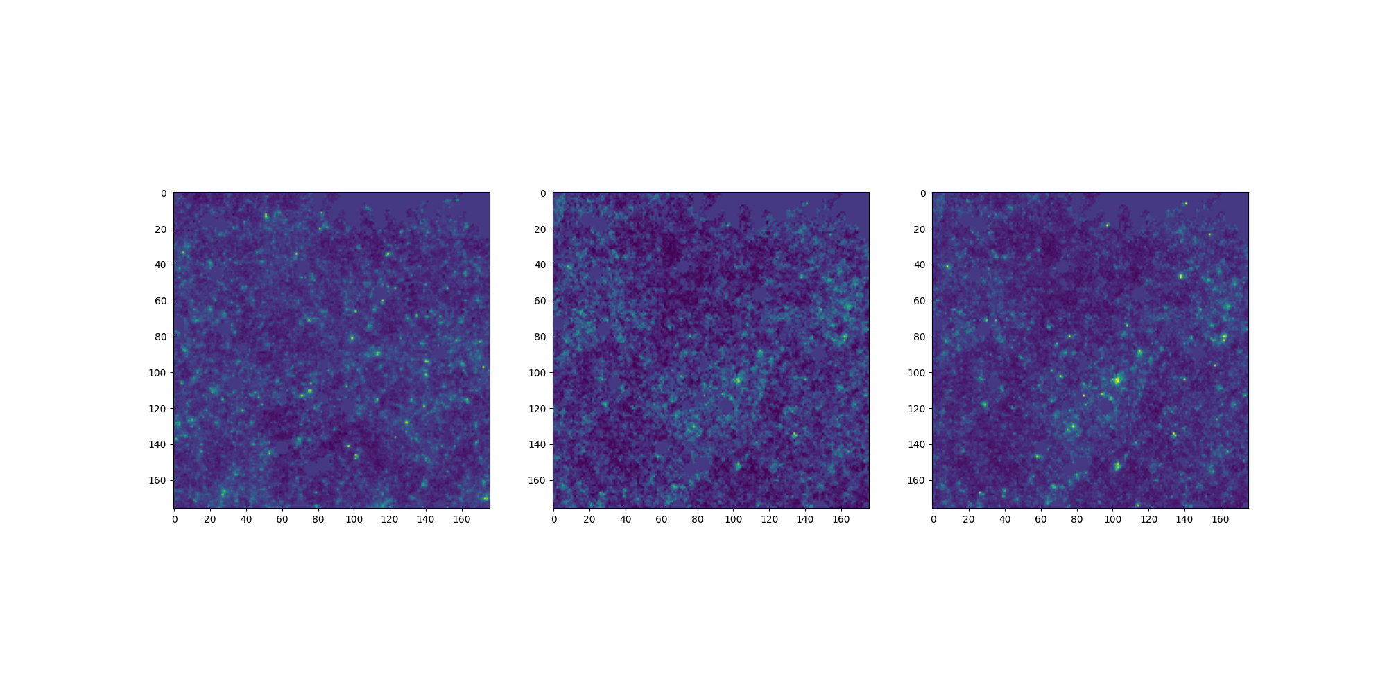
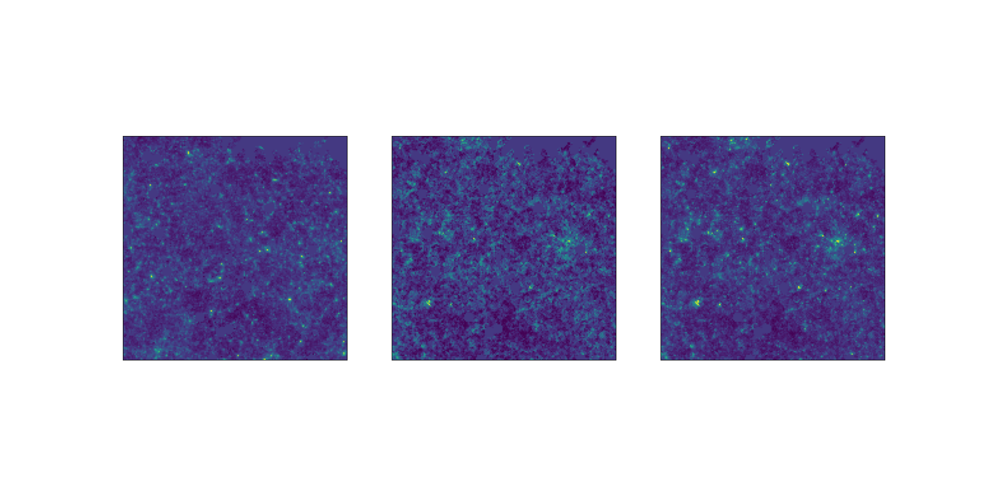
Dataset 1
Optimal Transport Plan
\pi(x_0, x_1)
Dataset 2
Requirements:
- has to map to a distribution sample.
\phi
- has to work in high dimensions.
\phi
- has to bridge any two distributions.
\phi
- has to bridge conditional distributions.
\phi
- has to be the solution of the OT problem.
\phi
✅
✅
✅
✅
✅
→ e.g. full nbody, hydro
\log p(x)
| O(ms) runtime | ✅ |
| differentiable | ✅ |
| ✅ | |
| realistic | ✅ |
\log p(x)
→ e.g. log-normal, LPT, PM
| O(ms) runtime | ✅ |
| differentiable | ✅ |
| ✅ | |
| realistic | ❌ |
Fast simulations
Emulated simulations
Results on weak lensing maps




LPT
PM
Learned
Residuals
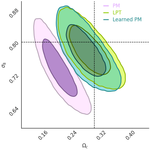
NeurIPS Challenge: Weak Lensing Uncertainty


LogNormal
Emulated

Challenge simulation
VS
NeurIPS Challenge: Weak Lensing Uncertainty
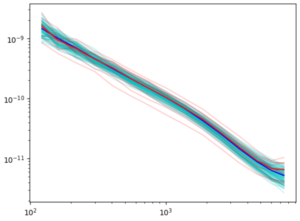
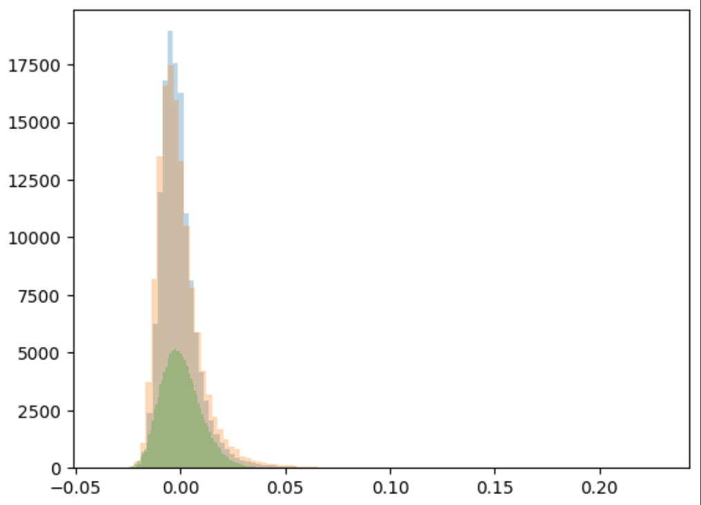
Power spectrum
LogNormal
Emulated
Challenge simulation
VS
NeurIPS Challenge: Weak Lensing Uncertainty

🥳
LogNormal
Emulated
Challenge simulation
VS
NeurIPS Challenge: Weak Lensing Uncertainty
Thank you for your attention!
SkAI FL Meeting
By Justine Zgh