Isospectral flows and a Casimir preserving scheme for long-time simulation of 2D hydrodynamics

Klas Modin

Collaborator: Milo Viviani

Euler equations of ideal hydrodynamics

\dot v + \nabla_v v = -\nabla p
\operatorname{div} v = 0

Leonhard Euler

Make sense on any Riemannian manifold

What is the generic

long-time behaviour?

3D

Nothing known, not even existence (related to Millenium problem)

Some things known:

inverse energy cascade

[Kraichnan 1967]

Various hypotheses based on statistical mechanics

2D

Motivation

Holy grail of 2D incompressible hydrodynamics:

  • Inner workings of the inverse energy cascade
  • Long-time behavior of mean-flow condensates

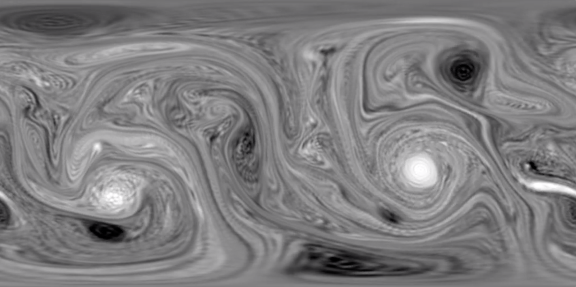
Zonal jet and vortex structures on Jupiter

Copyright: NASA, Cassini Imaging Team

Vorticity formulation

\dot v + \nabla_v v = -\nabla p
\operatorname{div} v = 0
\dot\omega + \{\omega,\psi \} = 0
\Delta\psi = \omega
v = \nabla^\bot\psi

Apply \(\operatorname{curl}\) to

\dot\omega + L_v\omega = 0

Vorticity \(\omega\) transported along \(v\)

Point-vortex dynamics (PVD):

invariant set of weak solutions

\displaystyle\omega = \sum_{k=1}^N p_k \delta_{q^k}

Conservation of Casimirs

\displaystyle \mathcal C_f(\omega) = \int f(\omega)

Statistical mechanics theories for 2D Euler

Idea by Onsager (1949):

  • Approximate \(\omega\) by PV for large \(N\)
  • Find invariant measure and presume ergodicity

Miller (1990) and Robert & Sommeria (1991): (MRS)

  • Minimize microcanonical entropy under energy and Casimir constraints

Predicts equilibrium of large-scale vortex structures

Is the MRS prediction correct?

No!

2D Euler equations are not ergodic

...but perhaps MRS is "generically" correct

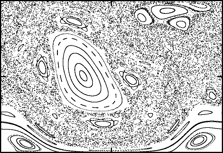
Flow ergodic except at "KAM islands"

Poincaré section of finite dimensional Hamiltonian system

Test MRS theory: a problem

for geometric integration

We need to:

  • Run long simulations
  • Preserve the Casimirs
    (energy + enstrophy alone not enough)
  • Preserve the Lie-Poisson structure

(criterion in MRS)

On \(\mathbb{T}^2\) such discretization exists (sine-bracket)

[Zeitlin 1991, McLachlan 1993]

based on quantization theory by Hoppe (1989)

Numerical simulations support MRS on \(\mathbb{T}^2\)

[Abramov & Majda 2003]

The torus is not a sphere

MRS generally assumed valid also on \(S^2\)

However, non-structure preserving simulations by Dritschel, Qi, & Marston (2015) contradict MRS on \(S^2\)

DQM simulation yield persistent unsteadiness

Our mission: construct trustworthy discretization on \(S^2\)

2D Euler to isospectral flow via Berezin-Toeplitz quantization

C^\infty(M)\ni f \mapsto T^N_f \in \mathfrak{g}_N

Exists if \(M\) compact quantizable Kähler manifold

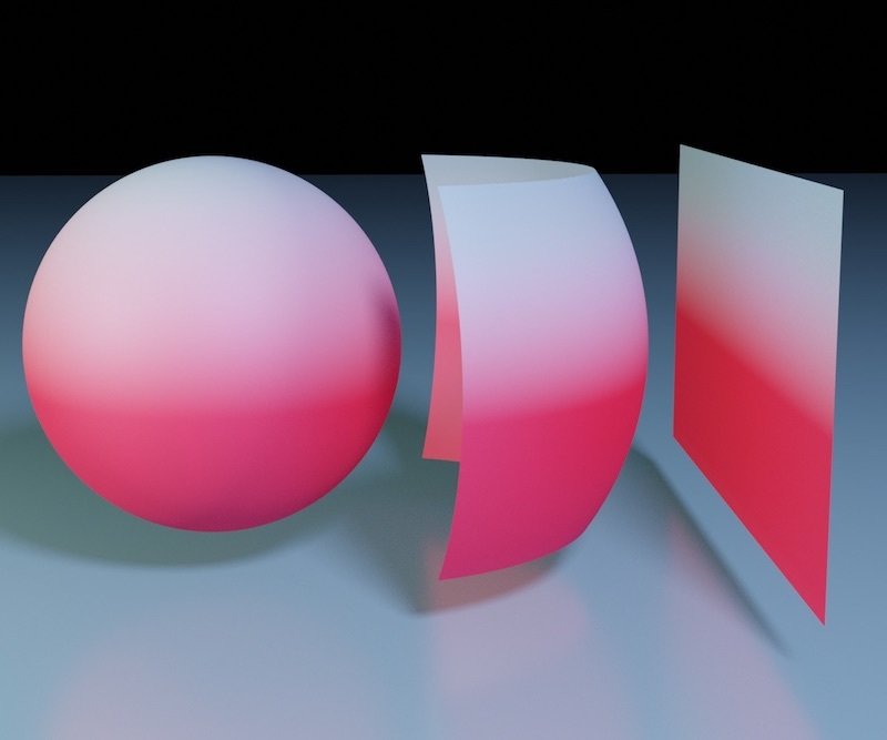
Idea: approximate Poisson algebra with matrix algebras

\{f,g\} \to [T^N_f,T^N_g] \quad N\to\infty
\displaystyle\dot \omega = \left\{\Delta^{-1}\omega,\omega \right\}
\displaystyle\dot W = [\Delta_N^{-1}W,W]

From 2D Euler

To isospectral

\omega \mapsto W

Lie-Poisson isospectral flows

\dot W = [B(W),W]

Let \(B\colon\mathfrak{g}\to\mathfrak{g}\)

isospectral flow

Analytic function \(f\) yields first integral

C_f(W) := \mathrm{tr}(f(W))

Casimir function

Hamiltonian case

B(W) = \nabla H(W)^\dagger

Hamiltonian function

Note: Non-canonical Poisson structure (Lie-Poisson)

Explicit B-T quantization on \(S^2\)

C^\infty(\mathbb S^2)\ni \omega\mapsto W \in \mathfrak{su}(N)

[Hoppe, 1989]

  • Express \(\omega\) in spherical harmonics expansion \[ \omega = \sum_{l=1}^\infty \sum_{m=-l}^l \omega^{lm}Y_{lm}\]
  • Truncate at \(l_{\it max}=N-1\)
  • For fixed \(m\), linear map between \((\omega^{lm})_{l=1}^{N-m})\) and \(m\):th diagonal of \(W\)
  • Gives \(N\) linear maps

Complicated coefficients, expressed by Wigner 3-j symbols of very high order

~2 weeks to compute coefficients for \(N=1025\)

Discrete \(S^2\) Laplacian on \(\mathfrak{su}(N)\)

  • "Magic" formula [Hoppe & Yau, 1998]
    \[\Delta_N W =\frac{N^2-1}{2}\left([X^N,[X^N,W]]- \frac{1}{2}[X_+^N,[X_-^N,W]]- \frac{1}{2}[X_-^N,[X_+^N,W]] \right)  \]

banded matrices

\displaystyle\dot W = [\Delta_N^{-1}W,W]

Recall

What is \(\Delta_N\) and how compute \(\Delta_N^{-1}W\) ?

(Naive approach requires \(O(N^3)\) operations with large constant)

\(O(N^2)\) operations

  • \(\Delta_N\) admits sparse \(LU\)-factorization with \(O(N^2\) non-zeros

Spatial discretization obtained!

\displaystyle \dot W = [\Delta_N^{-1}W,W]

Note: corresponds to

\(N^2\) spherical harmonics

\(O(N^2)\) operations

\(O(N^3)\) operations

Isospectral flow \(\Rightarrow\) discrete Casimirs

\displaystyle C^N_f(W) = \operatorname{tr}(f(W))

Time discretization

Aim: numerical integrator that is

  • isospectral, \(W_{k}\to W_{k+1}\) an isospectral map
    necessary to preserve Casimirs
     
  • symplectic, \(W_{k}\to W_{k+1}\) a Lie-Poisson map \(\mathfrak{su}(N)^*\to\mathfrak{su}(N)^*\)
    necessary to (nearly) preserve energy and phase space structure

What about symplectic Runge-Kutta methods (SRK)?

  • Not Lie-Poisson preserving!
  • Not isospectral!

Isospectral Symplectic

Runge-Kutta methods

[M. & Viviani 2019]

\dot W = [B(W),W]

Given \(s\)-stage Butcher tableau \((a_{ij},b_i)\) for SRK

\begin{aligned} X_i &= - (W_n + \sum_{j=1}^s a_{ij}X_j)h B(\tilde W_i) \\ Y_i &= hB(\tilde W_i)(W_k + \sum_{j=1}^sa_{ij}Y_j \\ K_{ij} &= h B(\tilde W_i)(\sum_{j'=1}^s(a_{ij'}X_{j'}+a_{jj'}K_{ij'})) \\ \tilde W_i &= W_k + \sum_{j=1}^s a_{ij}(X_j + Y_j + K_{ij} \\ W_{k+1} &= W_k + \sum_{i=1}^s [hB(\tilde W_i),\tilde W_i] \end{aligned}

Theorem: method is isospectral and Lie-Poisson preserving on any reductive Lie algebra

Numerical results

Same initial conditions as Dritschel, Qi, & Marston (2015)

\(N=501\)

Let's run it fast...

Strong numerical evidence against MRS!

Alignment with

point-vortex dynamics

Other initial conditions

What are "generic" initial conditions?

Our interpretation: sample from Gaussian random fields on \(H^1(S^2)\)

Non-zero angular momentum

\(N=501\)

Mechanism for long-time behaviour

Observation: large scale motion quasiperiodic

Assumptions for new mechanism:

  1. Small formations merge to larger (inverse energy cascade)
  2. Well-separated blobs interact approximately by PVD
  3. Dynamics is not integrable \(\Rightarrow\) blobs continue to merge
  4. \(k\)-PVD integrable \(\Rightarrow\) quasi-periodicity prevents further mixing

Integrability of PVD on \(S^2\)

Known since long: \(k\)-PVD integrable for \(k\leq 3\)

What about the 4-blob formations?

4-PVD on \(S^2\) non-integrable in general, but integrable for zero-momentum [Sakajo 2007]

Aref (2007) on PVD:

"a classical mathematics playground"

"many strands of classical mathematical physics come together"


Predictions for Euler on \(S^2\)

For generic initial conditions:

  1. Momentum small \(\Rightarrow\) 4-PVD is KAM-integrable \(\Rightarrow\) expect 4 non-steady vortex blobs
     
  2. Momentum intermediate \(\Rightarrow\) 3-PVD is integrable \(\Rightarrow\) expect 3 non-steady vortex blobs
     
  3. Momentum large \(\Rightarrow\) expect 2 large and 1 small vortex blobs

What's next?


  • Estimates on vortex blob dynamics vs. PVD
    [Caglioti, Lions, Marchioro, Pulvirenti, ...]
  • Quasi-periodic Euler solutions as perturbations of integrable PDE, infinite-dim KAM theory
    [Kuksin, ...]
  • Quantization as approach to "weak diffeomorphisms"
  • Rotating case (Coriolis parameters)
  • ...
  • Convergence of the model

Conjecture [M. & Viviani, 2020]
Fixed interval \([0,T]\), constant \(C=C(T,\omega_0)\) s.t. \[ \sup |\omega(t,\cdot)-T_N^{-1}(W^N(t)| \leq C/N \]

Thank you!

Isospectral flows and a Casimir preserving scheme for long-time simulation of 2D hydrodynamics

By Klas Modin

Isospectral flows and a Casimir preserving scheme for long-time simulation of 2D hydrodynamics

Presentation given 2020-02 at PCTS in Princeton. This presentation is more technical than the one given in Bonn.

  • 1,296