


Klas Modin PRO
Mathematician at Chalmers University of Technology and the University of Gothenburg
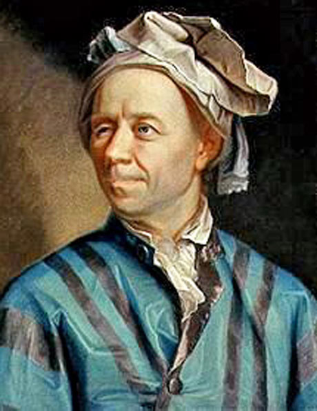
Leonhard Euler
Make sense on any Riemannian manifold
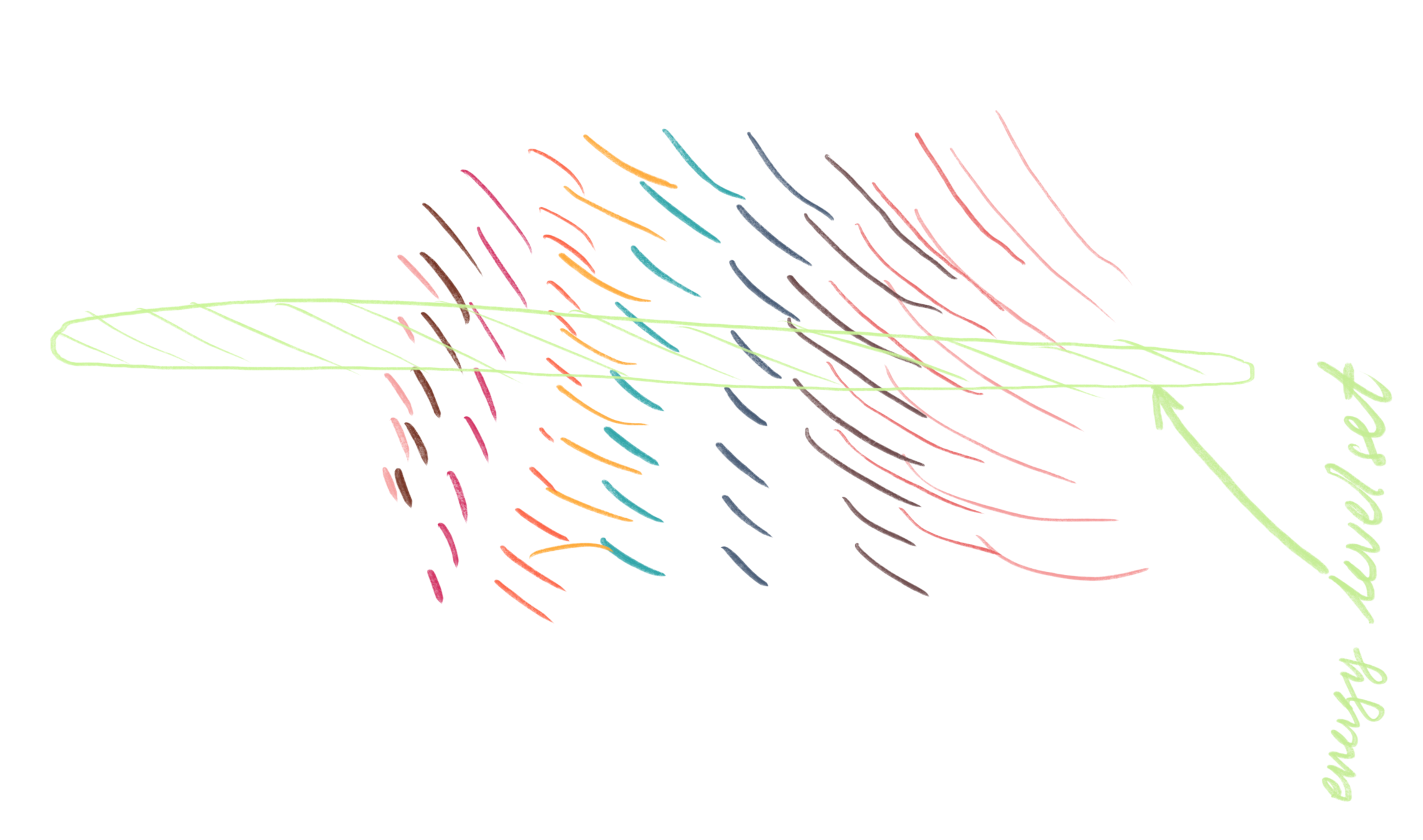
Apply curl to \(v\)
level-sets of \(\omega\)
Lie-Poisson system on \(\mathfrak{X}_\mu(S^2)^* \simeq C^\infty_0(S^2) \)
\(G=\mathrm{Diff}_\mu(S^2)\)
\(T_e^*G\simeq\mathfrak g^*\)
Casimir functions:
Finite-dim (weak) co-adjoint orbits:
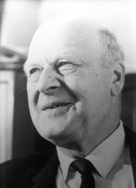
Idea by Onsager (1949):
Hamiltonian function:
Idea by Onsager (1949):
Hamiltonian function:
Onsager's observation:
Pos. and neg. strengths \(\Rightarrow\) energy takes values \(-\infty\) to \(\infty\)
Idea by Onsager (1949):
Hamiltonian function:
Onsager's observation:
Pos. and neg. strengths \(\Rightarrow\) energy takes values \(-\infty\) to \(\infty\)
\(\Rightarrow\) phase volume function \(v(E)\) has inflection point
Idea by Onsager (1949):
Hamiltonian function:
Miller (1990) and Robert & Sommeria (1991): (MRS)
2D Euler equations are not ergodic
...but perhaps MRS is "generically" correct
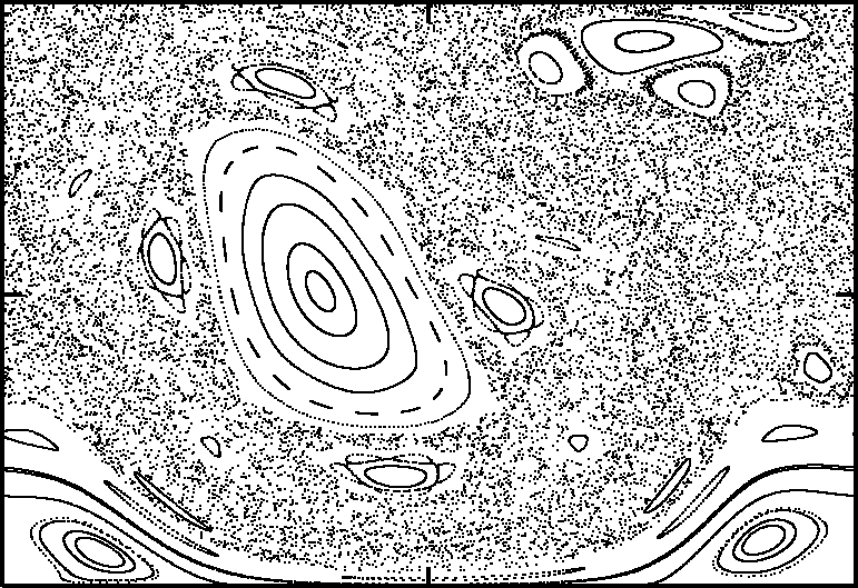
Flow ergodic except at "KAM islands"
Poincaré section of finite dimensional Hamiltonian system
To test MRS we need to:
(criterion in MRS)
On \(\mathbb{T}^2\) such discretization exists (sine-bracket)
[Zeitlin 1991, McLachlan 1993]
based on quantization theory by Hoppe (1989)
[Abramov & Majda 2003]
MRS generally assumed valid also on \(S^2\)
However, non-structure preserving simulations by Dritschel, Qi, & Marston (2015) contradict MRS on \(S^2\)
DQM simulation yield persistent unsteadiness
Our mission: trustworthy discretization on \(S^2\)
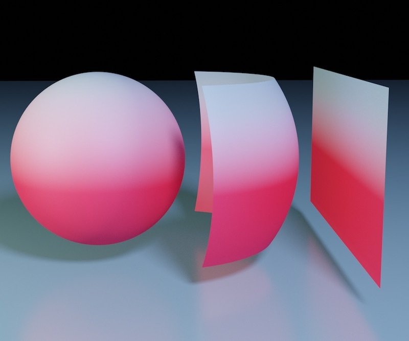
Exists if \(M\) compact quantizable Kähler manifold
Idea: approximate Poisson algebra with matrix algebras
From 2D Euler
To isospectral
Let \(B\colon\mathfrak{g}\to\mathfrak{g}\)
isospectral flow
Analytic function \(f\) yields first integral
Casimir function
Hamiltonian case
Hamiltonian function
Note: Non-canonical Poisson structure (Lie-Poisson)
[Hoppe, 1989]
Complicated coefficients, expressed by Wigner 3-j symbols of very high order
~2 weeks to compute coefficients for \(N=1025\)
banded matrices
Recall
What is \(\Delta_N\) and how compute \(\Delta_N^{-1}W\) ?
(Naive approach requires \(O(N^3)\) operations with large constant)
\(O(N^2)\) operations
Note: corresponds to
\(N^2\) spherical harmonics
\(O(N^2)\) operations
\(O(N^3)\) operations
Isospectral flow \(\Rightarrow\) discrete Casimirs
Aim: numerical integrator that is
What about symplectic Runge-Kutta methods (SRK)?
[M. & Viviani 2019]
Given \(s\)-stage Butcher tableau \((a_{ij},b_i)\) for SRK
Theorem: method is isospectral and Lie-Poisson preserving on any reductive Lie algebra
Evolution of quantized vorticity with \(N=501\)
Let's run it fast...
Strong numerical evidence against MRS!
What are "generic" initial conditions?
Our interpretation: sample from Gaussian random fields on \(H^{1+\epsilon}(S^2)\)
Non-zero angular momentum
\(N=501\)
Observation: large scale motion quasiperiodic
Assumptions for new mechanism:
Known since long: \(k\)-PVD integrable for \(k\leq 3\)
What about the 4-blob formations?
4-PVD on \(S^2\) non-integrable in general, but integrable for zero-momentum [Sakajo 2007]
Aref (2007) on PVD:
"a classical mathematics playground"
"many strands of classical mathematical physics come together"
For generic initial conditions:
By Klas Modin
Presentation given 2021-02 at the Mathematics Colloquium of Florida State University.


