


Klas Modin PRO
Mathematician at Chalmers University of Technology and the University of Gothenburg
Def: momentum map \(J: T^*Q\to \mathfrak{g}^* \) for cotangent lifted action
Proposition: gradient flow is
Simplest special case: right-invariant metric \[ \mathcal G_{e}(\xi,\xi) = \langle \mathcal A\xi,\xi\rangle, \qquad \mathcal A:\mathfrak g\to\mathfrak g^*\]
Proposition: gradient flow on \(\mathrm{Orb}_G(q_0)\) is
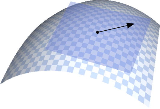
\(\mathcal G\) induces metric \(\bar{\mathcal G}\) on \(\mathrm{Orb}_G(q_0)\)
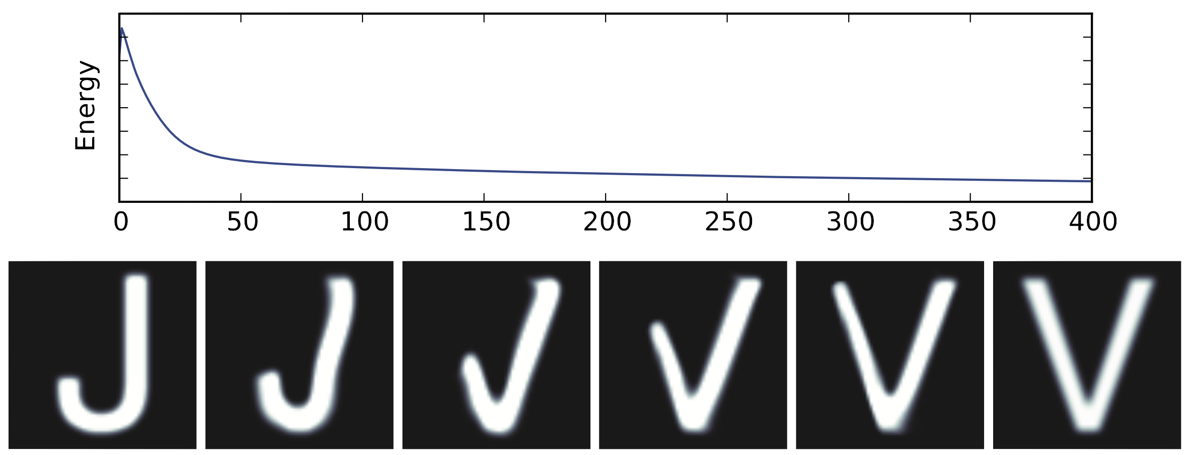
Typical form
distance or divergence
Gradient flow
Lie-Euler method
Guides object-oriented design of shape analysis software
horizontal slice
fiber
fiber
\(QR\) example
\(QR\) example
\(QR\) example
Right action of \(\mathrm{GL}(n)\) on \(P(n)\) is transitive
\(QR\) example
\(QR\) example
Notice: no regularization used here
\(QR\) example
\(QR\) example
Convexity lemma:
Corollary:
\(QR\) example
\(QR\) example
\(QR\) example
Brockett example
Brockett example
Proposition: Fisher-Rao gradient flow restricted to orbits is
Corollary: Expressed in \(\Sigma = W^{-1}\) we get
Double bracket form of Brockett's flow
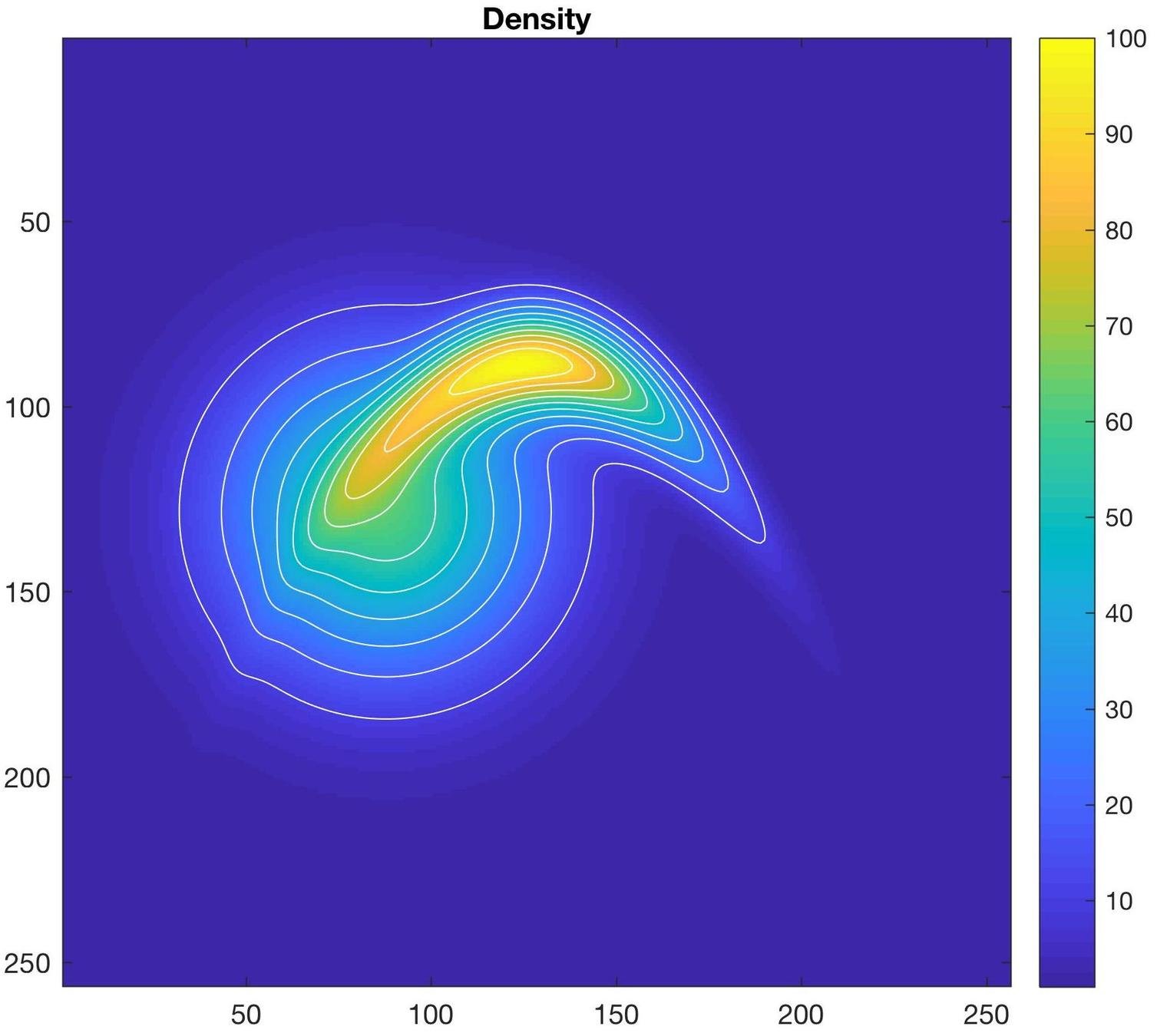
Density example
lots of structure!
(with M. Bauer and S. Joshi)
\(H^1\) metric
Fisher-Rao metric = explicit geodesics
Density example
Gradient flow on orbits of \(\mathrm{Dens}(M)\times\mathrm{Dens}(M)\)
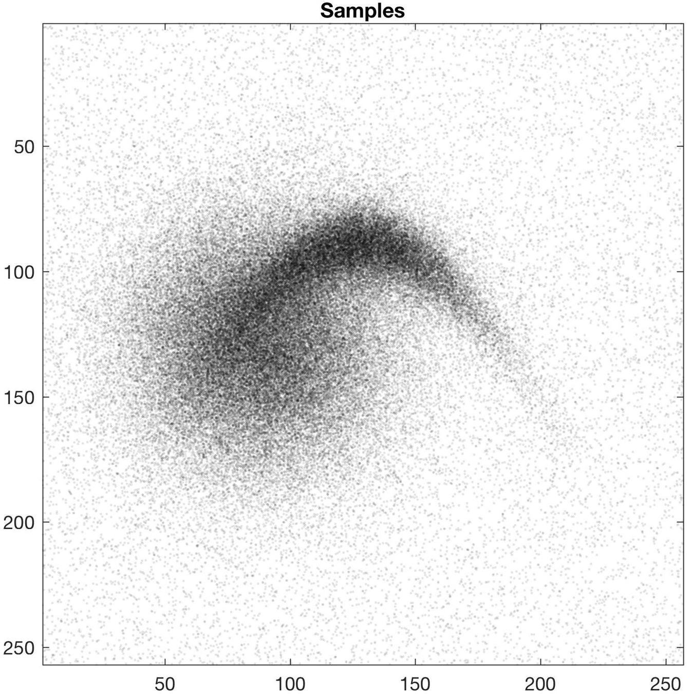
Problem 1: given \(\mu\in\mathrm{Dens}(M)\) generate \(N\) samples from \(\mu\)
Most cases: use Monte-Carlo based methods
Special case here:
transport map approach
might be useful
Density example
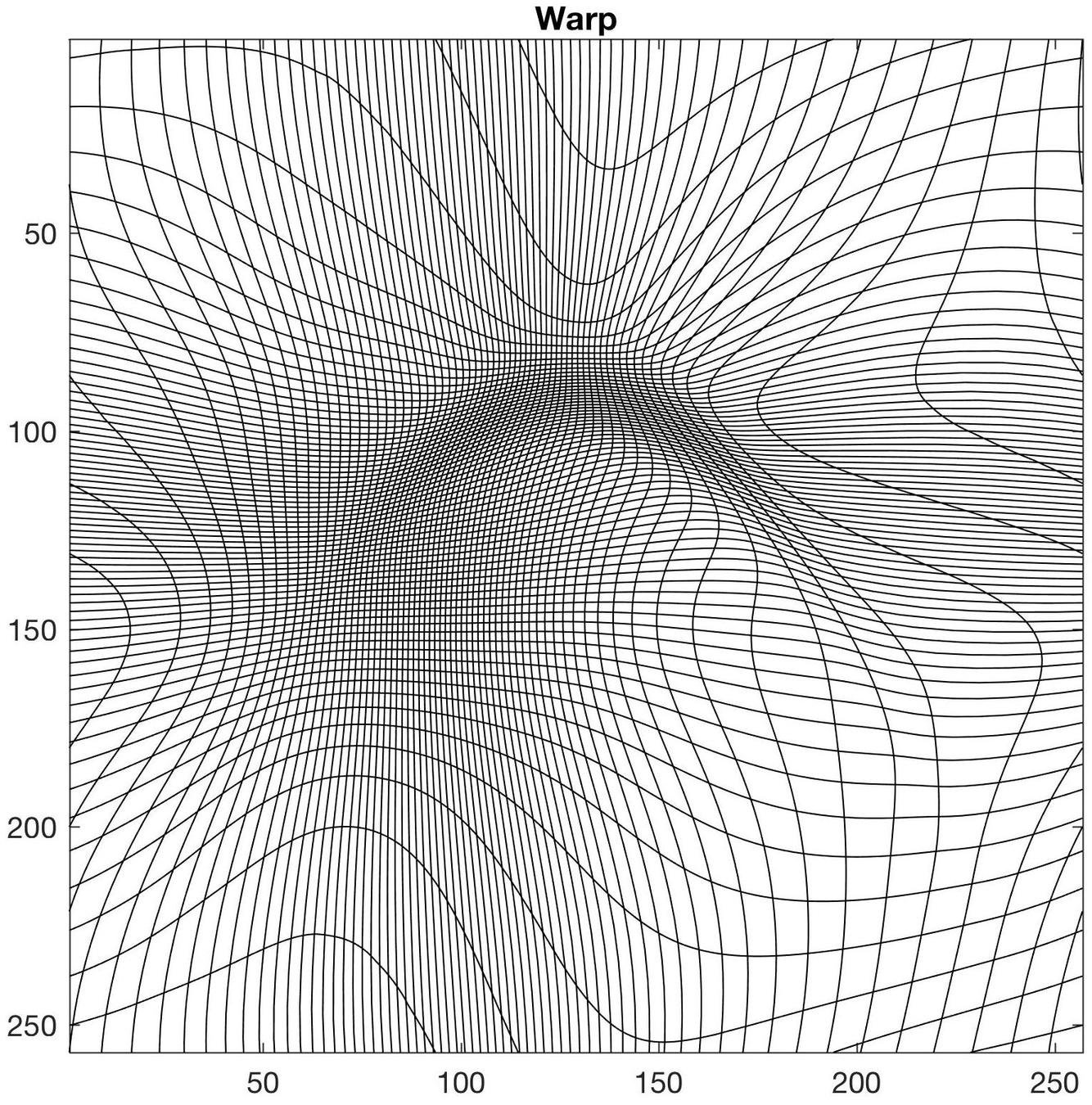
Problem 2: given \(\mu\in\mathrm{Dens}(M)\) find \(\varphi\in\mathrm{Diff}(M)\) minimizing
under constraint \(\varphi_*\mu_0 = \mu\)
Studied case: (Moselhy and Marzouk 2012, Reich 2013, ...)
Our notion:
Density example
Warp computation time (256*256 gridsize, 100 time-steps): ~1s
Sample computation time (10^7 samples): < 1s
Density example
\(\rho_0\)
\(\rho_1\)
Density example
\(\rho_0\)
\(\rho_1\)
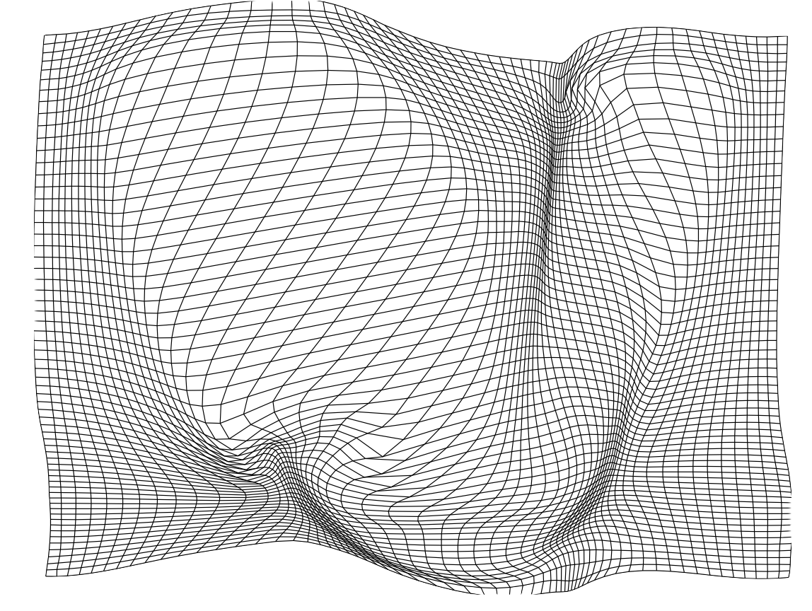
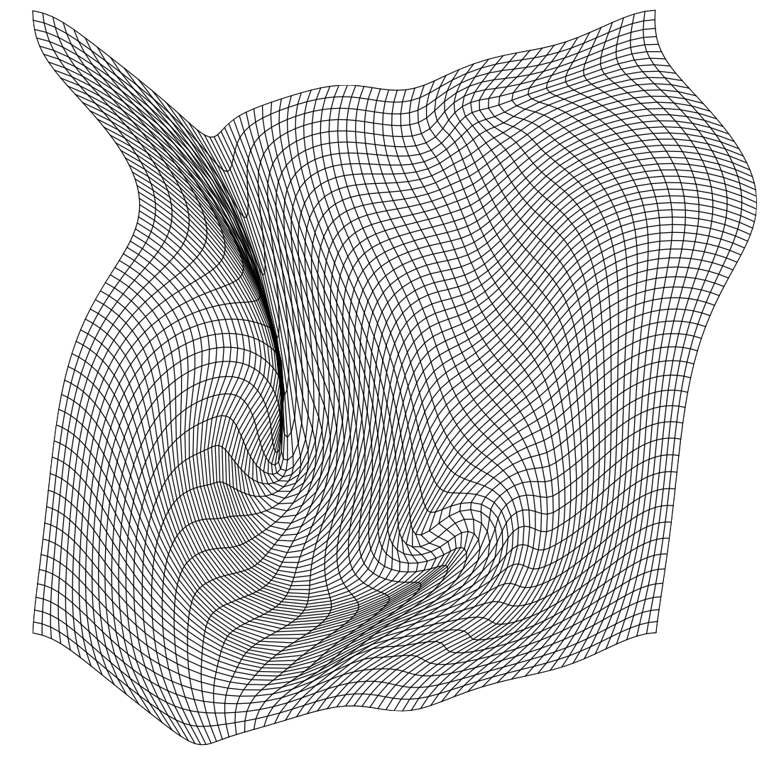
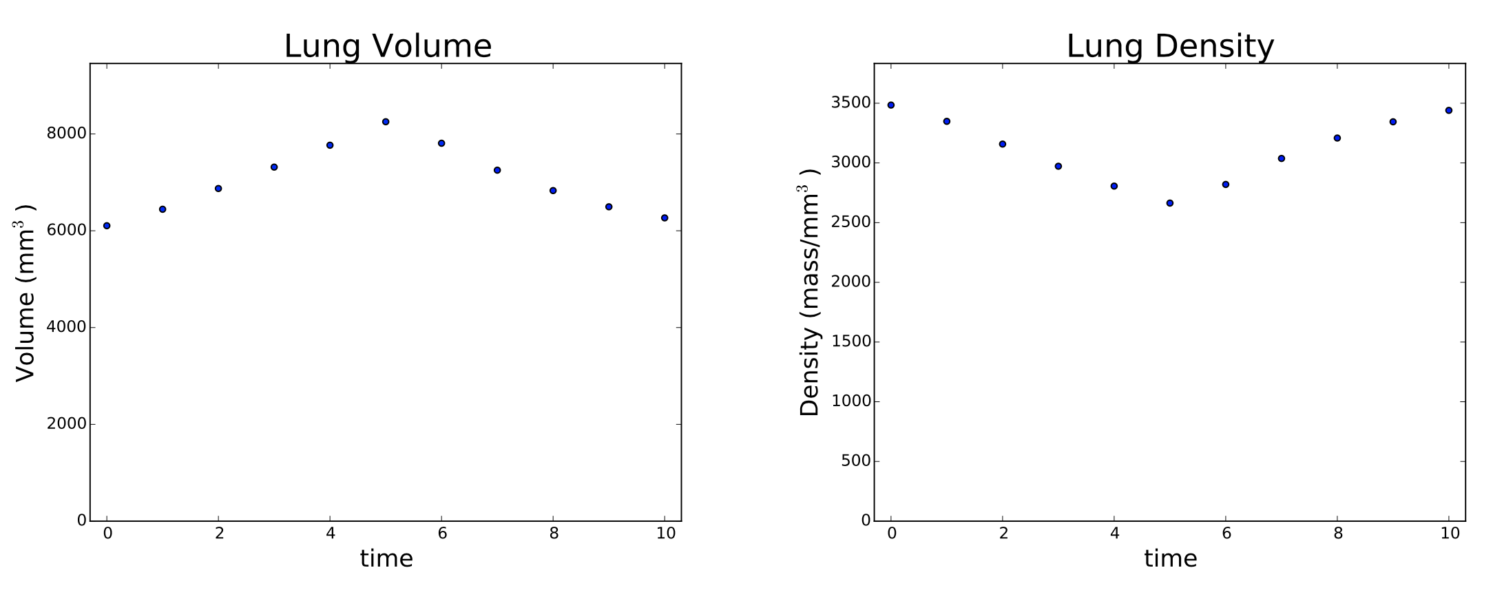
Density example
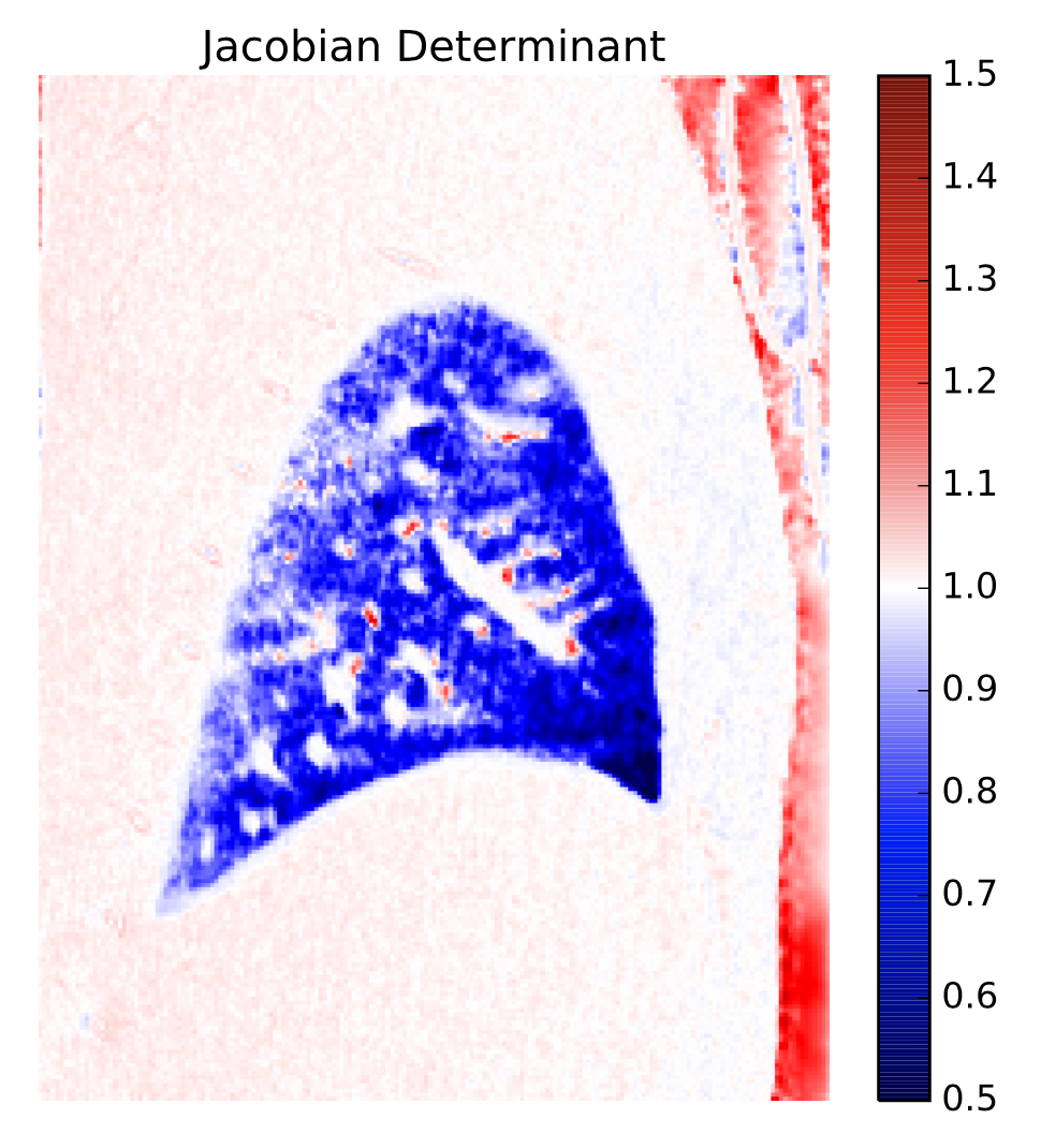
Data: breathing cycle of rat, CT imaging
Density example
Regularized density flow
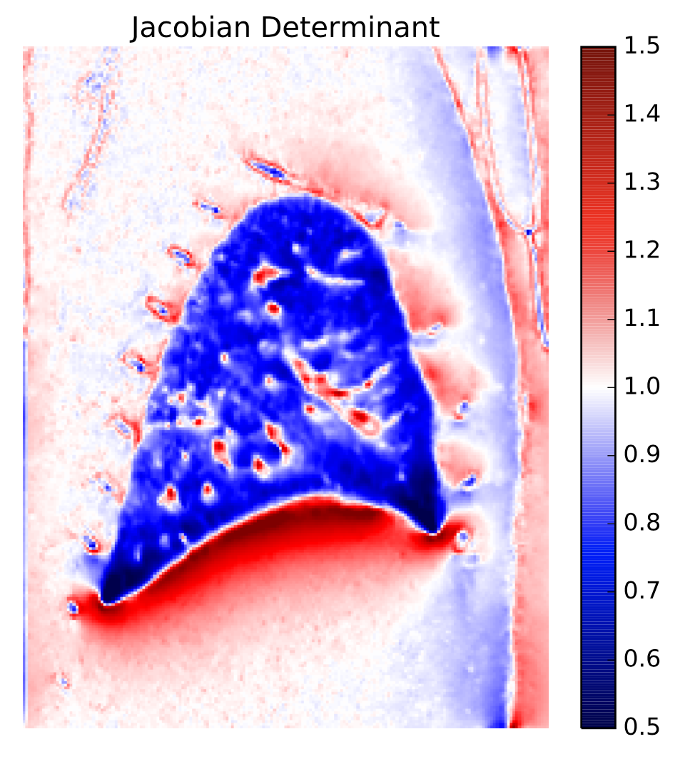
LDDMM
Density example
LDDMM example
Why is LDDMM computationally expensive?
Because \( \frac{\delta d^2_\mathcal A(\mathrm{id},\cdot)}{\delta \eta}\) is expensive
LDDMM example
explicit formula (cf. Peter's talk)
(cf. Joshi, Pennec, and others)
deformation
tensor
Gradient flow on orbit in \(C^\infty(M)\times\mathrm{Met}(M)\)
LDDMM example
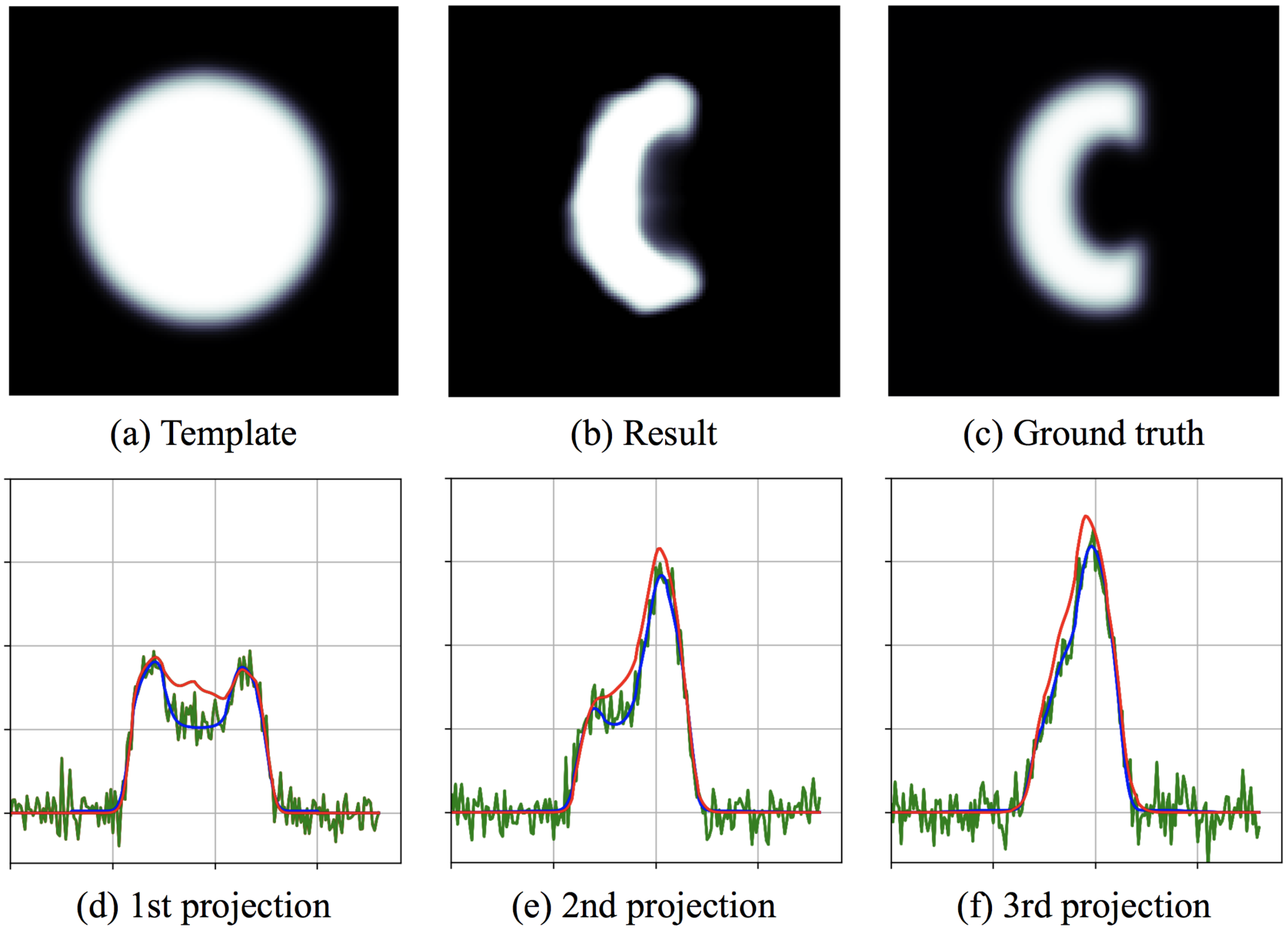
Reconstruction example
(with O. Öktem)
Reconstruction example
Gradient flow on orbit in \(\mathrm{Dens}(M)\times\mathrm{Met}(M)\)
Reconstruction example
References
Slides available at: slides.com/kmodin
By Klas Modin
Presentation given 2017-11-13 at the Isaac Newton Institute in Cambridge.


