


lucasw
大佬教麻
你可以叫我 000 / Lucas
建國中學資訊社37th學術長
建國中學電子計算機研習社44th學術
校際交流群創群者
不會音遊不會競程不會數學的笨
資訊技能樹亂點但都一樣爛
專案爛尾大師
IZCC x SCINT x Ruby Taiwan 聯課負責人
建國中學電子計算機研習社44th學術+總務
是的,我是總務。在座的你各位下次記得交社費束脩給我
技能樹貧乏
想拿機器學習做專題結果只學會使用API
上屆社展烙跑到資訊社的叛徒
科班墊神
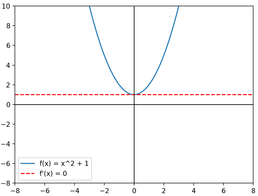
\(f(x)=ax^2+bx+c\)
\(f'(x)=2ax^1+bx\)
\(y=b_0+b_1x\)
?
\(\hat y=b_0+b_1x\)
殘差平方和最小
\((x_1,y_1),(x_2,y_2)...(x_n,y_n)\)
\(\hat y = b_0 + b_1x\)
\(\hat y_1 - y_1 = (b_0 + b_1x_1) - y_1\)
\(\sum_{i=1}^{n} (\hat y_i - y_i)^2\)
用一個函數來計算誤差
ex.
MAE(Mean Absolute Error)
MSE(Mean Square Error)
cross-entropy
還有其他各式各樣的
\(L = \sum_{i=1}^{n} (\hat y_i - y_i)^2\)
\(= \sum_{i=1}^{n} (b_0 + b_1x_i-y_i)^2\)
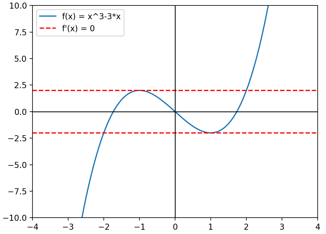
\(f'(x)=0\)
\(x\)
梯度=\(f'(x)\)
\(x'\)
\(x' = x - f'(x)\)
\(x' = x -\alpha f'(x)\)
超參數(hyperparameter)
\(L = \sum_{i=1}^{n} (\hat y_i - y_i)^2\)
\(= \sum_{i=1}^{n} (b_0 + b_1x_i-y_i)^2\)
\(\frac{\partial L}{\partial b_0}=0\)
\(\frac{\partial L}{\partial b_1}=0\)
\(f(x) = (b_0+b_1x-y)^2\)
\(\frac {\partial}{\partial b_0}(b_0+b_1x-y)^2\) ?
\(\frac{dy}{dx}=\frac{dy}{du} \frac{du}{dx}\)
\(y = (x+1)^2\)
令 \(u=x+1\)
\(\frac{dy}{dx}=\frac{dy}{du} \frac{du}{dx}=\frac{(x+1)^2}{x+1} \frac{x+1}{x}\)
\(\frac{dy}{dx}=\frac{dy}{du} \frac{du}{dx}=\frac{(x+1)^2}{x+1} \frac{x+1}{x}\)
\(\frac{dy}{du}=2(x+1)\)
\(\frac{du}{dx}=1\)
\(\frac{dy}{dx}=2(x+1) \times 1=2x+2\)
\(f(x) = (b_0+b_1x-y)^2\)
\(\frac {\partial}{\partial b_0}f(x)=\frac{\partial f(x)}{\partial u}\frac{\partial u}{\partial b_0}\)
令 \(u=b_0+b_1x-y\)
\(\frac{\partial}{\partial b_0}f(x)=2(b_0+b_1x-y) \times 1\)
\(\frac{\partial}{\partial b_0}f(x)=2(\hat y-y)\)
\(f(x) = (b_0+b_1x-y)^2\)
\(\frac {\partial}{\partial b_1}f(x)=\frac{\partial f(x)}{\partial u}\frac{\partial u}{\partial b_1}\)
令 \(u=b_0+b_1x-y\)
\(\frac{\partial}{\partial b_1}=2(b_0+b_1x-y)\times x\)
\(\frac{\partial}{\partial b_1}=2(\hat y-y)\times x\)
import random
import numpy as np
import matplotlib.pyplot as plt
from mpl_toolkits.mplot3d import Axes3D

def MSE(b_0, b_1):
    loss = 0
    for i in range(len(x)):
        y_hat= b_0 + b_1 * x[i]
        loss += (y_hat- y[i])**2
    return loss / len(x)

def gradient_0(b_0, b_1):
    gradient = 0
    for i in range(len(x)):
        y_hat= b_0 + b_1 * x[i]
        gradient += 2 * (y_hat- y[i]) / len(x)
    return gradient

def gradient_1(b_0, b_1):
    gradient = 0
    for i in range(len(x)):
        y_hat= b_0 + b_1 * x[i]
        gradient += 2 * (y_hat- y[i]) * x[i] / len(x)
    return gradient

# y_hat= 0.5 * x - 5
random.seed(114514)
x = [i for i in range(-50, 50, 1)]
y = [0.5 * i - 5 + random.randint(-10, 10) for i in x]
b_0_history = []
b_1_history = []
loss_history = []

#起始位置
b_0 = -15
b_1 = 0.2

#hyperparameter
epoch = 10
lr = 0.001 #別超過0.0015

#梯度下降
for i in range(epoch):
    b_0_history.append(b_0)
    b_1_history.append(b_1)
    loss_history.append(MSE(b_0, b_1))
    b_0 -= lr*gradient_0(b_0, b_1)
    b_1 -= lr*gradient_1(b_0, b_1)

# 定義 b_0_axis 和 b_1_axis 的範圍
b_0_axis = np.linspace(-20, 10, 100)
b_1_axis = np.linspace(0, 1, 100)

# 創建網格
b_0_axis, b_1_axis = np.meshgrid(b_0_axis, b_1_axis)
Loss_values = np.zeros_like(b_0_axis)

# 計算每個 (b_0_axis, b_1_axis) 對應的 Loss 值
for i in range(b_0_axis.shape[0]):
    for j in range(b_0_axis.shape[1]):
        Loss_values[i, j] = MSE(b_0_axis[i, j], b_1_axis[i, j])

# 繪製三維圖
fig = plt.figure(figsize=(10, 7))
ax = fig.add_subplot(111, projection='3d')
ax.plot_surface(b_0_axis, b_1_axis, Loss_values, cmap='viridis', alpha=0.8)

# 繪製梯度下降路徑
ax.plot(b_0_history, b_1_history, loss_history,"o-", color='red')

# 添加標籤
ax.set_xlabel('b_0_axis')
ax.set_ylabel('b_1_axis')
ax.set_zlabel('Loss(b_0_axis, b_1_axis)')
ax.legend()

# 顯示圖形
plt.show()
import random
import numpy as np
import matplotlib.pyplot as plt
from mpl_toolkits.mplot3d import Axes3D
def MSE(b_0, b_1):
loss = 0
for i in range(len(x)):
y_hat= b_0 + b_1 * x[i]
loss += (y_hat- y[i])**2
return loss / len(x)
def gradient_0(b_0, b_1):
gradient = 0
for i in range(len(x)):
y_hat= b_0 + b_1 * x[i]
gradient += 2 * (y_hat- y[i]) / len(x)
return gradient
def gradient_1(b_0, b_1):
gradient = 0
for i in range(len(x)):
y_hat= b_0 + b_1 * x[i]
gradient += 2 * (y_hat- y[i]) * x[i] / len(x)
return gradient
# y_hat= 0.5 * x - 5
random.seed(114514)
x = [i for i in range(-50, 50, 1)]
y = [0.5 * i - 5 + random.randint(-10, 10) for i in x]
b_0_history = []
b_1_history = []
loss_history = []
#起始位置
b_0 = -15
b_1 = 0.2
#hyperparameter
epoch = 10
lr = 0.001 #別超過0.0015
#梯度下降
for i in range(epoch):
b_0_history.append(b_0)
b_1_history.append(b_1)
loss_history.append(MSE(b_0, b_1))
b_0 -= lr*gradient_0(b_0, b_1)
b_1 -= lr*gradient_1(b_0, b_1)
# 定義 b_0_axis 和 b_1_axis 的範圍
b_0_axis = np.linspace(-20, 10, 100)
b_1_axis = np.linspace(0, 1, 100)
# 創建網格
b_0_axis, b_1_axis = np.meshgrid(b_0_axis, b_1_axis)
Loss_values = np.zeros_like(b_0_axis)
# 計算每個 (b_0_axis, b_1_axis) 對應的 Loss 值
for i in range(b_0_axis.shape[0]):
for j in range(b_0_axis.shape[1]):
Loss_values[i, j] = MSE(b_0_axis[i, j], b_1_axis[i, j])
# 繪製三維圖
fig = plt.figure(figsize=(10, 7))
ax = fig.add_subplot(111, projection='3d')
ax.plot_surface(b_0_axis, b_1_axis, Loss_values, cmap='viridis', alpha=0.8)
# 繪製梯度下降路徑
ax.plot(b_0_history, b_1_history, loss_history,"o-", color='red')
# 添加標籤
ax.set_xlabel('b_0_axis')
ax.set_ylabel('b_1_axis')
ax.set_zlabel('Loss(b_0_axis, b_1_axis)')
ax.legend()
# 顯示圖形
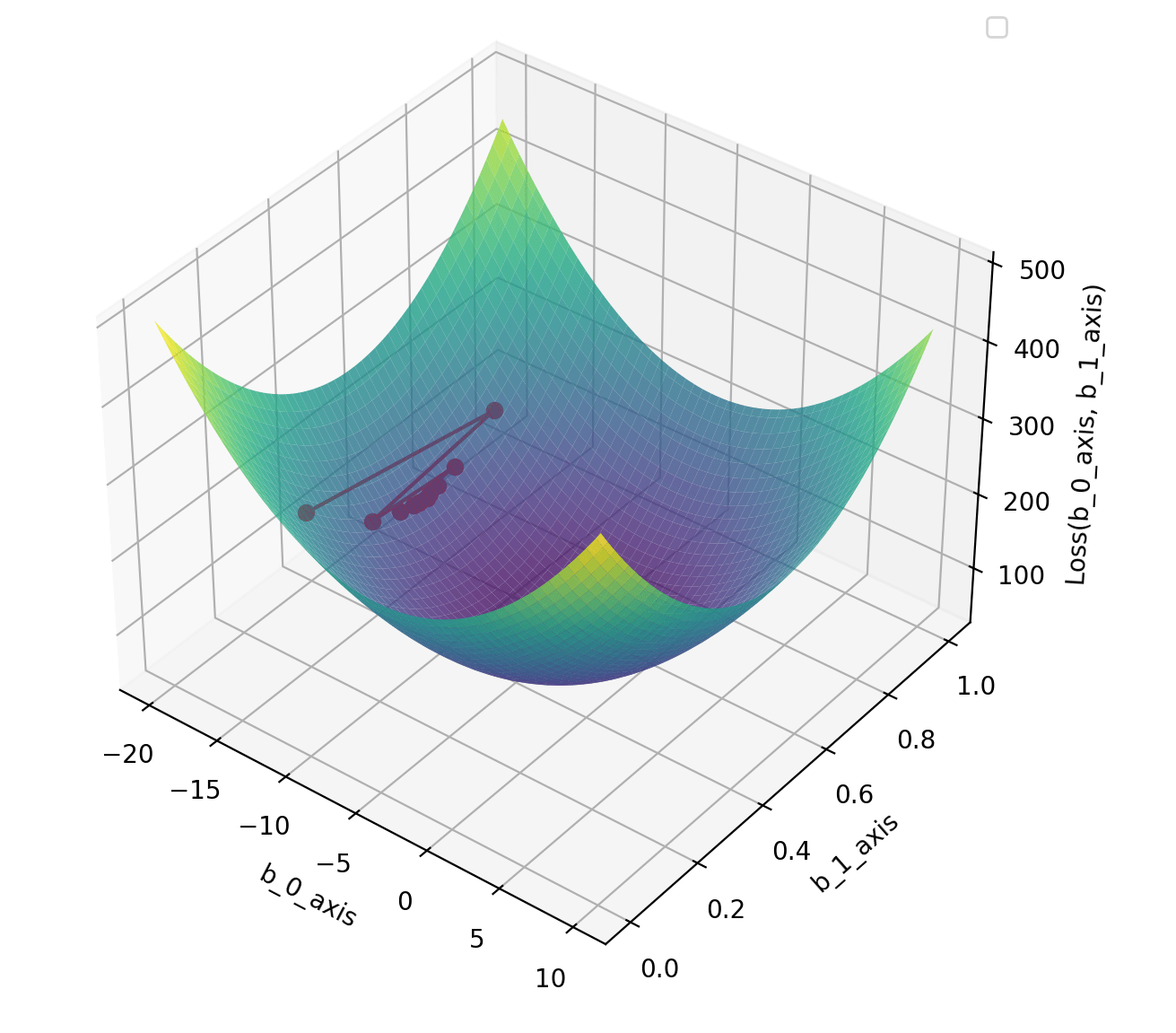
plt.show()MSE=\(\frac{1}{n} \sum_{i=1}^{n} (b_0 + b_1x_i-y_i)^2\)
import random
import numpy as np
import matplotlib.pyplot as plt
from mpl_toolkits.mplot3d import Axes3D

def MSE(b_0, b_1):
    loss = 0
    for i in range(len(x)):
        y_hat= b_0 + b_1 * x[i]
        loss += (y_hat- y[i])**2
    return loss / len(x)

def gradient_0(b_0, b_1):
    gradient = 0
    for i in range(len(x)):
        y_hat= b_0 + b_1 * x[i]
        gradient += 2 * (y_hat- y[i]) / len(x)
    return gradient

def gradient_1(b_0, b_1):
    gradient = 0
    for i in range(len(x)):
        y_hat= b_0 + b_1 * x[i]
        gradient += 2 * (y_hat- y[i]) * x[i] / len(x)
    return gradient

# y_hat= 0.5 * x - 5
random.seed(114514)
x = [i for i in range(-50, 50, 1)]
y = [0.5 * i - 5 + random.randint(-10, 10) for i in x]
b_0_history = []
b_1_history = []
loss_history = []

#起始位置
b_0 = -15
b_1 = 0.2

#hyperparameter
epoch = 10
lr = 0.001 #別超過0.0015

#梯度下降
for i in range(epoch):
    b_0_history.append(b_0)
    b_1_history.append(b_1)
    loss_history.append(MSE(b_0, b_1))
    b_0 -= lr*gradient_0(b_0, b_1)
    b_1 -= lr*gradient_1(b_0, b_1)

# 定義 b_0_axis 和 b_1_axis 的範圍
b_0_axis = np.linspace(-20, 10, 100)
b_1_axis = np.linspace(0, 1, 100)

# 創建網格
b_0_axis, b_1_axis = np.meshgrid(b_0_axis, b_1_axis)
Loss_values = np.zeros_like(b_0_axis)

# 計算每個 (b_0_axis, b_1_axis) 對應的 Loss 值
for i in range(b_0_axis.shape[0]):
    for j in range(b_0_axis.shape[1]):
        Loss_values[i, j] = MSE(b_0_axis[i, j], b_1_axis[i, j])

# 繪製三維圖
fig = plt.figure(figsize=(10, 7))
ax = fig.add_subplot(111, projection='3d')
ax.plot_surface(b_0_axis, b_1_axis, Loss_values, cmap='viridis', alpha=0.8)

# 繪製梯度下降路徑
ax.plot(b_0_history, b_1_history, loss_history,"o-", color='red')

# 添加標籤
ax.set_xlabel('b_0_axis')
ax.set_ylabel('b_1_axis')
ax.set_zlabel('Loss(b_0_axis, b_1_axis)')
ax.legend()

# 顯示圖形
plt.show()import random
import numpy as np
import matplotlib.pyplot as plt
from mpl_toolkits.mplot3d import Axes3D
def MSE(b_0, b_1):
loss = 0
for i in range(len(x)):
y_hat= b_0 + b_1 * x[i]
loss += (y_hat- y[i])**2
return loss / len(x)
def gradient_0(b_0, b_1):
gradient = 0
for i in range(len(x)):
y_hat= b_0 + b_1 * x[i]
gradient += 2 * (y_hat- y[i]) / len(x)
return gradient
def gradient_1(b_0, b_1):
gradient = 0
for i in range(len(x)):
y_hat= b_0 + b_1 * x[i]
gradient += 2 * (y_hat- y[i]) * x[i] / len(x)
return gradient
# y_hat= 0.5 * x - 5
random.seed(114514)
x = [i for i in range(-50, 50, 1)]
y = [0.5 * i - 5 + random.randint(-10, 10) for i in x]
b_0_history = []
b_1_history = []
loss_history = []
#起始位置
b_0 = -15
b_1 = 0.2
#hyperparameter
epoch = 10
lr = 0.001 #別超過0.0015
#梯度下降
for i in range(epoch):
b_0_history.append(b_0)
b_1_history.append(b_1)
loss_history.append(MSE(b_0, b_1))
b_0 -= lr*gradient_0(b_0, b_1)
b_1 -= lr*gradient_1(b_0, b_1)
# 定義 b_0_axis 和 b_1_axis 的範圍
b_0_axis = np.linspace(-20, 10, 100)
b_1_axis = np.linspace(0, 1, 100)
# 創建網格
b_0_axis, b_1_axis = np.meshgrid(b_0_axis, b_1_axis)
Loss_values = np.zeros_like(b_0_axis)
# 計算每個 (b_0_axis, b_1_axis) 對應的 Loss 值
for i in range(b_0_axis.shape[0]):
for j in range(b_0_axis.shape[1]):
Loss_values[i, j] = MSE(b_0_axis[i, j], b_1_axis[i, j])
# 繪製三維圖
fig = plt.figure(figsize=(10, 7))
ax = fig.add_subplot(111, projection='3d')
ax.plot_surface(b_0_axis, b_1_axis, Loss_values, cmap='viridis', alpha=0.8)
# 繪製梯度下降路徑
ax.plot(b_0_history, b_1_history, loss_history,"o-", color='red')
# 添加標籤
ax.set_xlabel('b_0_axis')
ax.set_ylabel('b_1_axis')
ax.set_zlabel('Loss(b_0_axis, b_1_axis)')
ax.legend()
# 顯示圖形
plt.show()\(\frac{\partial L}{\partial b_0}=0\)
\(\frac{\partial L}{\partial b_1}=0\)
把數據線性壓縮到0~1之間
\(x_1,x_2,...x_n\)
\(x_i'=\frac{x_i-min(x_1,x_2,...,x_n)}{max(x_1,x_2,...,x_n)-min(x_1,x_2,...,x_n)}\)
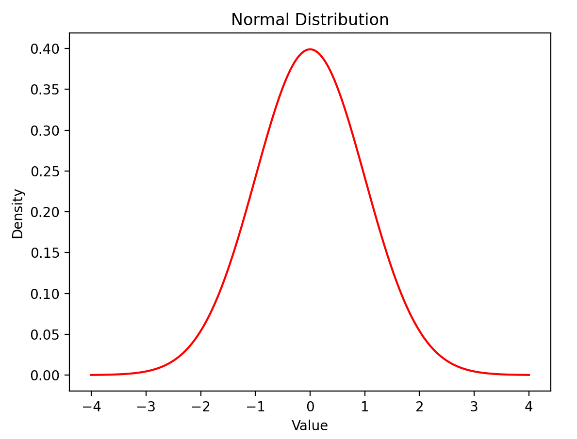
使平均值 = 0,標準差 = 1
\(x_1,x_2,...x_n\)
\(x_i'=\frac{x_i-\mu_x}{\sigma_x}\)
68%
96%
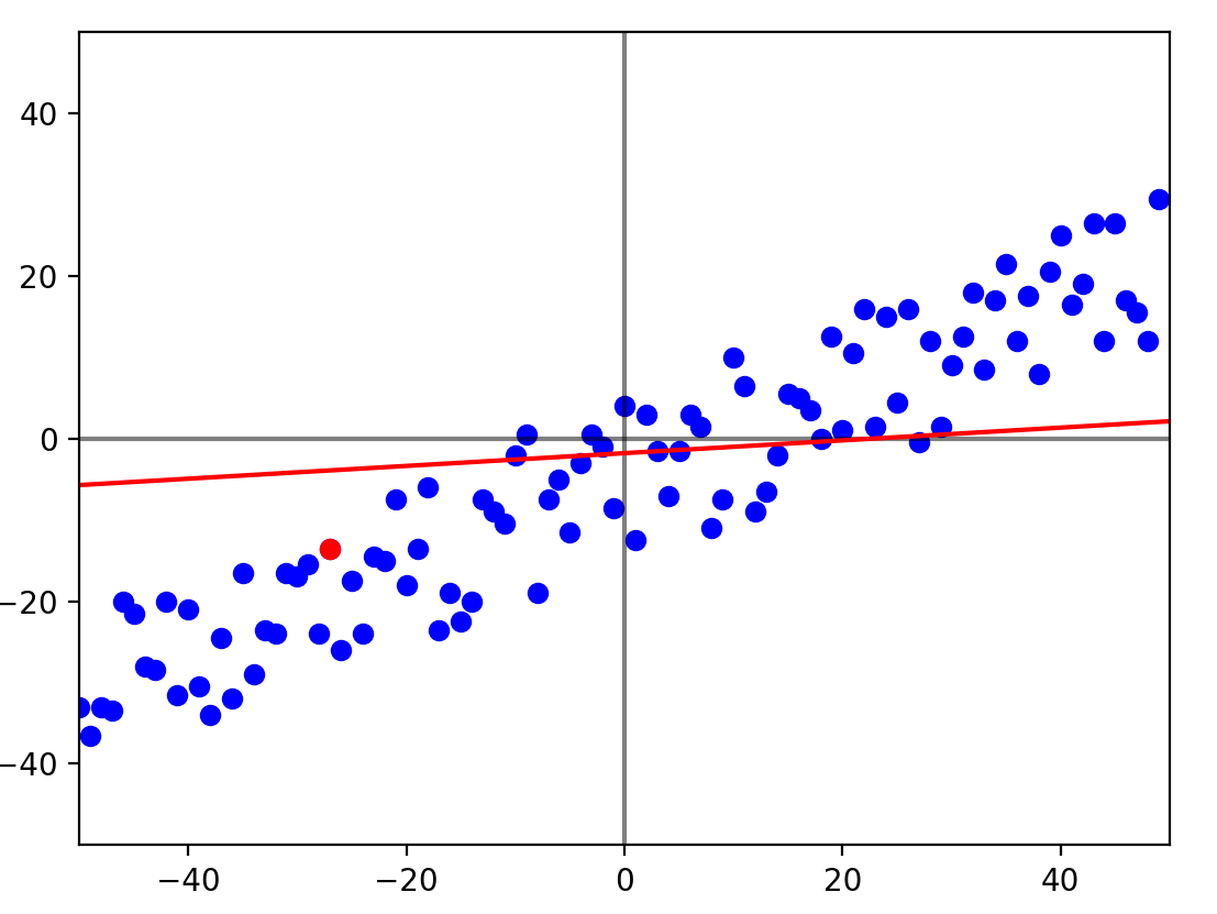
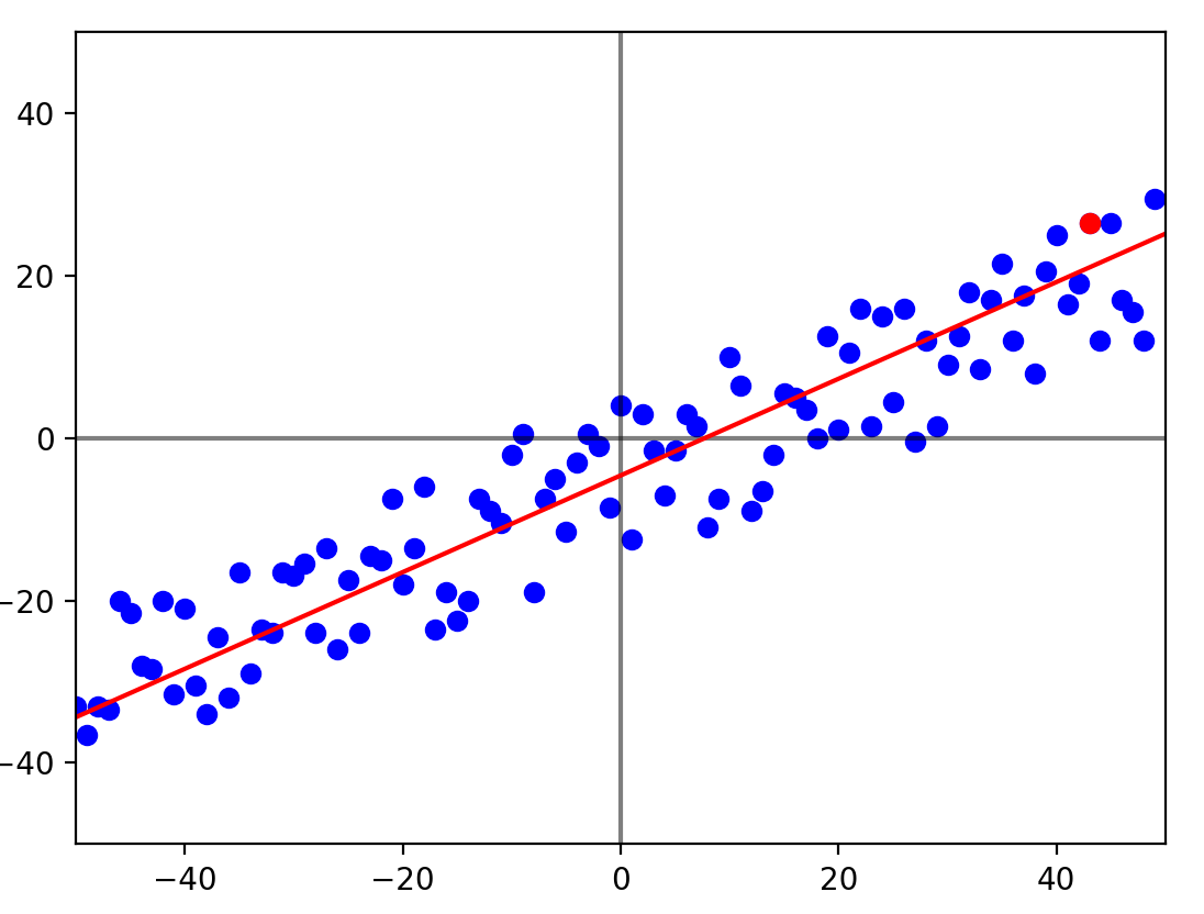
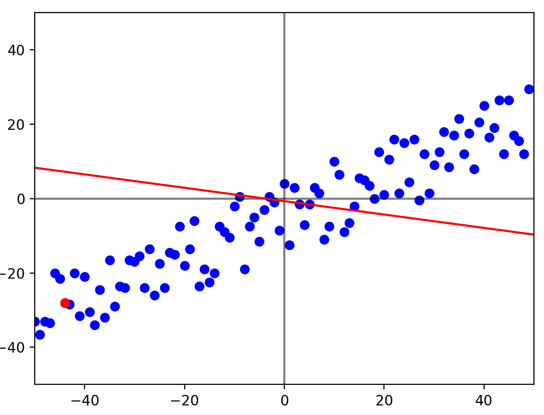
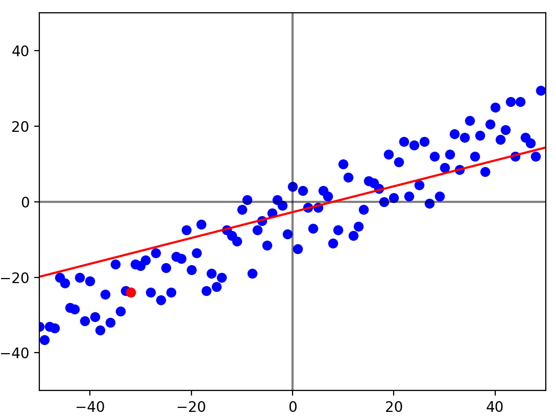
import random

import matplotlib.pyplot as plt
from IPython import display

# y = 0.5 * x - 5
random.seed(114514)
x = [i for i in range(-50, 50, 1)]
y = [0.5 * i - 5 + random.randint(-10, 10) for i in x]
b_0 = random.uniform(-1, 1)
b_1 = random.uniform(-1, 1)
print("before train:")
print(f"b_0:{b_0}")
print(f"b_1:{b_1}\n")

alpha_0 = 0.01
alpha_1 = 0.0001
epoch = 100

def f(x):
    return b_0 + b_1 * x

def delta_0(y, yh):
    return -2 * (y-yh)

def delta_1(y, yh, x):
    return -2 * (y-yh) * x

for _ in range(epoch):
    plt.clf()
    plt.plot([-50,50], [0,0], c="black", alpha=0.5)
    plt.plot([0,0], [-50,50], c="black", alpha=0.5)
    plt.xlim(-50, 50)
    plt.ylim(-50, 50)

    i = random.randint(0, 99)
    yh = b_0 + b_1 * x[i]
    b_0 -= alpha_0 * delta_0(y[i], yh)
    b_1 -= alpha_1 * delta_1(y[i], yh, x[i])
    plt.plot([-50, 50], [f(-50), f(50)], c="red")
    plt.scatter(x, y, c="blue")
    plt.scatter(x[i], y[i], c="red")
    plt.pause(0.01)
    display.clear_output(wait=True)

plt.pause(-1)
print("after train:")
print(f"b_0:{b_0}")
print(f"b_1:{b_1}")import random
import numpy as np
import matplotlib.pyplot as plt
from mpl_toolkits.mplot3d import Axes3D
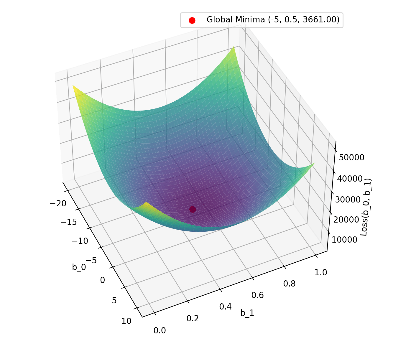
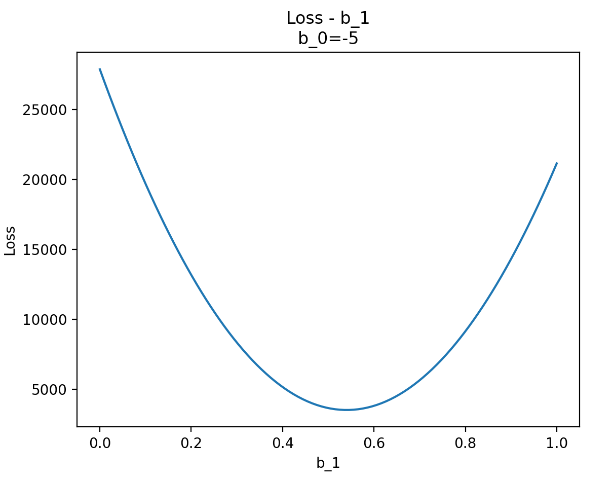
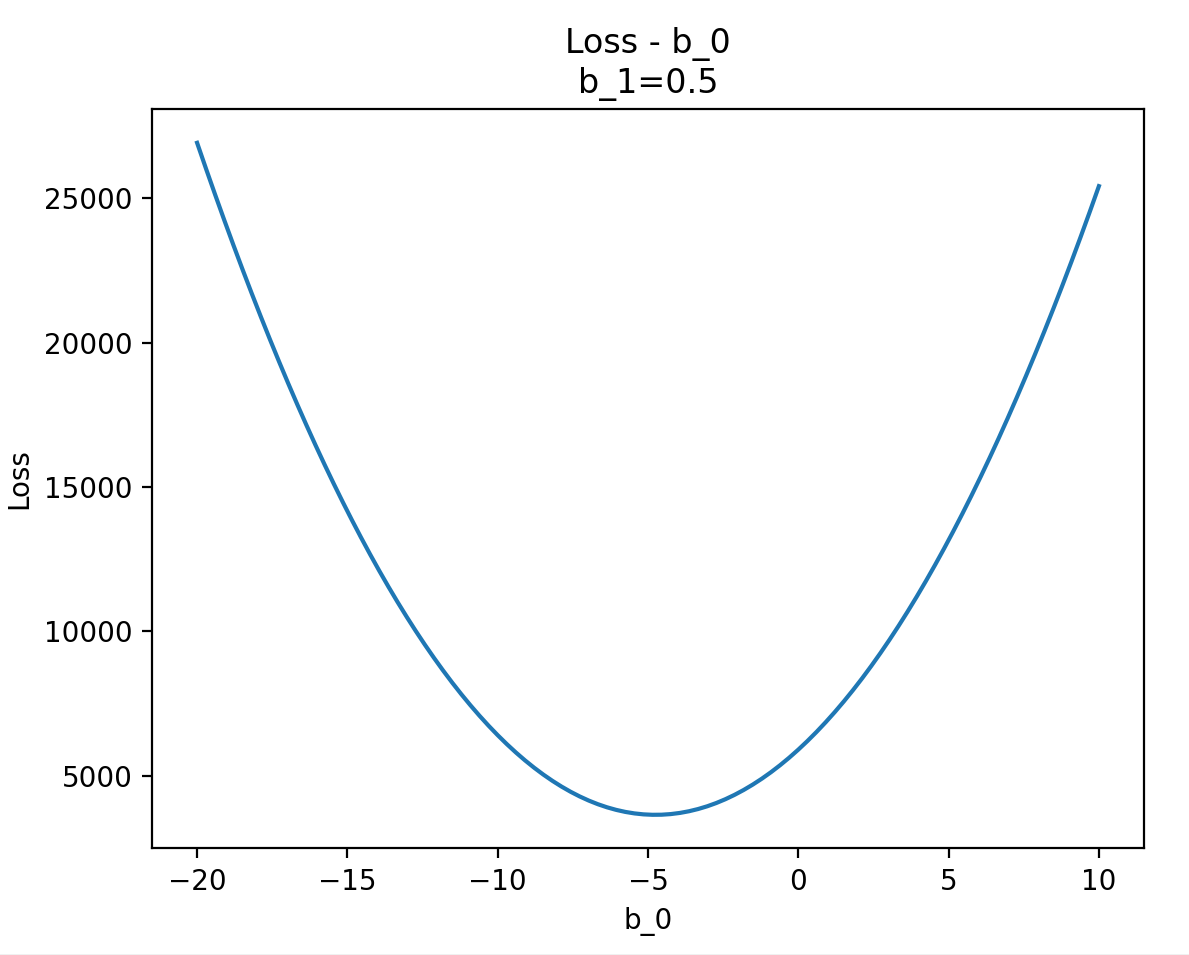
def Loss(b_0, b_1):
loss = 0
for i in range(len(x)):
y_hat = b_0 + b_1 * x[i]
loss += (y_hat - y[i])**2
return loss
# y_hat = 0.5 * x - 5
random.seed(114514)
x = [i for i in range(-50, 50, 1)]
y = [0.5 * i - 5 + random.randint(-10, 10) for i in x]
# 定義 b_0 和 b_1 的範圍
b_0 = np.linspace(-20, 10, 100)
b_1 = np.linspace(0, 1, 100)
# 創建網格
B_0, B_1 = np.meshgrid(b_0, b_1)
Loss_values = np.zeros_like(B_0)
# 計算每個 (b_0, b_1) 對應的 Loss 值
for i in range(B_0.shape[0]):
for j in range(B_0.shape[1]):
Loss_values[i, j] = Loss(B_0[i, j], B_1[i, j])
# 繪製三維圖
fig = plt.figure(figsize=(10, 7))
ax = fig.add_subplot(111, projection='3d')
ax.plot_surface(B_0, B_1, Loss_values, cmap='viridis', alpha=0.8)
# 添加紅點標記 b_0 = -5, b_1 = 0.5
b_0_point = -5
b_1_point = 0.5
loss_point = Loss(b_0_point, b_1_point)
ax.scatter(b_0_point, b_1_point, loss_point, color='red', s=50, label=f"Global Minima (-5, 0.5, {loss_point:.2f})")
# 添加標籤
ax.set_xlabel('b_0')
ax.set_ylabel('b_1')
ax.set_zlabel('Loss(b_0, b_1)')
ax.legend()
# 顯示圖形
plt.show()import matplotlib.pyplot as plt
import random
import numpy as np
from IPython import display
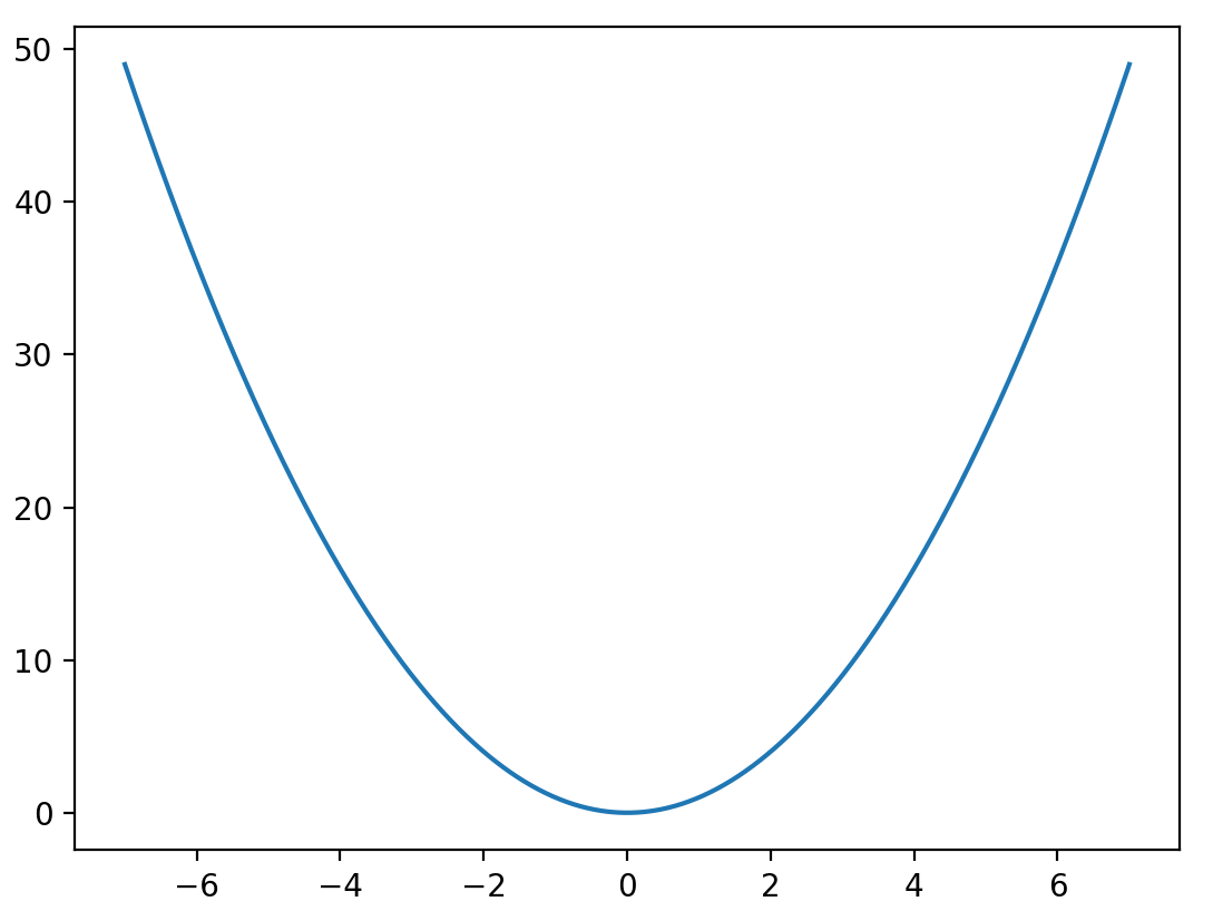
def f(x):
return 3*x**2
def df(x):
return 6*x
x = 3
lr = 0.3 #learning rate
step = 10
x_history = []
y_history = []
for i in range(step):
x_history.append(x)
y_history.append(f(x))
x -= lr*df(x)
X = np.linspace(-5,5,100)
plt.plot(X,f(X),"b-")
plt.plot(x_history,y_history,"o-",c="r")
plt.show()
#動畫
'''
for i in range(len(x_history)):
plt.clf()
X = np.linspace(-5,5,100)
plt.plot(X,f(X),"b-")
plt.plot(x_history[i],y_history[i],"o",c="r")
plt.pause(0.2)
display.clear_output(wait=True)
plt.pause(-1)
'''是的我們又要講數學了。
這就是每個Neuron在進行的事情
把輸入( X )乘上一個Weight並且加上Bias
最後在套上Activation Function
如果一直進行wx+b的操作會發現它始終是線性的,這樣一來這整個神經網路能夠擬合出來的函式會被限縮
並且能夠對每個神經元輸出的值進行一定程度的控制
例如: 限縮範圍,限縮負數成長
而激勵函數能夠提供給這個神經網路的方程式非線性的來改善這個問題
以下為幾種常見的激勵函數範例
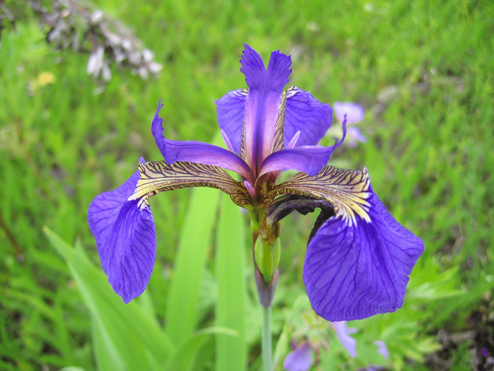
透過花瓣跟萼片分辨鳶尾花種類
經典分類問題
輸入:花瓣長寬+花萼長寬(4項)
輸出:鳶尾花種類(3種)
山鳶尾(setosa)
雜色鳶尾(vesicolor)
維吉尼亞鳶尾(virginica)
輸出一個機率
山鳶尾(setosa) => 1
雜色鳶尾(vesicolor) => 0
\(\hat y=\sigma(\vec X \cdot \vec W +b)\)
\(L = -\sum [y\ln (\hat y)+(1-y)\ln (1-\hat y)]\)
\(y\)是實際機率
\(\hat y\)是預估機率
\(\frac{\partial L}{\partial w_i}=\frac{\partial L}{\partial u}\frac{\partial u}{\partial w_i}\), \(u=x_i\times w_i+b\)
\(\frac{\partial L}{\partial u}=\frac{\partial L}{\partial \sigma(u)}\frac{\partial \sigma(u)}{\partial u}=\sum (\hat y-y)\)
\(\frac{\partial L}{\partial u}=\frac{\partial L}{\partial \hat y}\frac{\partial \hat y}{\partial u}\)
\(\frac{\partial L}{\partial u}=\frac{\partial L}{\partial \sigma (u)}\frac{\partial \sigma (u)}{\partial u}\)
\(\frac{\partial L}{\partial w_i}=\sum(\hat y_i-y_i)\times x_i\)
\(\frac{\partial L}{\partial w_i}=\sum(\hat y-y)\times\frac{\partial u}{\partial w_i}\), \(u=x_i\times w_i+b\)
\(\frac{\partial L}{\partial b}=\sum(\hat y-y)\times\frac{\partial u}{\partial b}\), \(u=x_i\times w_i+b\)
\(\frac{\partial L}{\partial b}=\sum(\hat y_i-y_i)\)
| id | 花萼長 | 花萼寬 | 花瓣長 | 花瓣寬 | 品種 |
|---|---|---|---|---|---|
| 1 | 5.1 | 3.5 | 1.4 | 0.2 | Iris-setosa |
| 2 | 4.9 | 3.0 | 1.4 | 0.2 | Iris-setosa |
| ... | ... | ... | ... | ... | ... |
| 150 | 5.9 | 3.0 | 5.1 | 1.8 | Iris-virginica |
setosa
versicolor
virginica
id
1~50
51~100
101~150
| id | 花萼長 | 花萼寬 | 花瓣長 | 花瓣寬 | 品種 |
|---|---|---|---|---|---|
| 1 | 5.1 | 3.5 | 1.4 | 0.2 | Iris-setosa |
| 2 | 4.9 | 3.0 | 1.4 | 0.2 | Iris-setosa |
| ... | ... | ... | ... | ... | ... |
| 100 | 5.7 | 2.8 | 4.1 | 1.3 | Iris-versicolor |
setosa
versicolor
id
1~50
51~100
| id | 花萼長 | 花萼寬 | 花瓣長 | 花瓣寬 | Label |
|---|---|---|---|---|---|
| 1 | 5.1 | 3.5 | 1.4 | 0.2 | 1 |
| 2 | 4.9 | 3.0 | 1.4 | 0.2 | 1 |
| ... | ... | ... | ... | ... | ... |
| 100 | 5.7 | 2.8 | 4.1 | 1.3 | 0 |
setosa => 1
versicolor => 0
id
1~50
51~100
| 花萼長 | 花萼寬 | 花瓣長 | 花瓣寬 | Label |
|---|---|---|---|---|
| 5.1 | 3.5 | 1.4 | 0.2 | 1 |
| 4.9 | 3.0 | 1.4 | 0.2 | 1 |
| ... | ... | ... | ... | ... |
| 5.7 | 2.8 | 4.1 | 1.3 | 0 |
setosa => 1
versicolor => 0
1~50
51~100
| 花萼長 | 花萼寬 | 花瓣長 | 花瓣寬 | Label |
|---|---|---|---|---|
| 5.0 | 2.3 | 3.3 | 1.0 | 0 |
| 5.1 | 3.8 | 1.9 | 0.4 | 1 |
| ... | ... | ... | ... | ... |
| 4.7 | 3.2 | 1.6 | 0.2 | 1 |
setosa => 1
versicolor => 0
y = data[:,4].reshape(-1,1)
| 花萼長 | 花萼寬 |
|---|---|
| 5.0 | 2.3 |
| 5.1 | 3.8 |
| ... | ... |
| 4.7 | 3.2 |
| Label |
|---|
| 0 |
| 1 |
| ... |
| 1 |
x = data[:,0:2]
y = data[:,4].reshape(-1,1)
x = data[:,0:2]
W = np.random.randn(2,1)
b = np.random.randn(1)
\(\hat y=\sigma(\vec X \cdot \vec W +b)\)
\(-\sum [y\ln (\hat y)+(1-y)\ln (1-\hat y)]\)
\(\hat y=\sigma(\vec X \cdot \vec W +b)\)
\(\hat y=\sigma(\vec X \cdot \vec W +b)\)
\(\hat y=\sigma(\vec X \cdot \vec W +b)\)
\(\hat y=\sigma(\vec X \cdot \vec W +b)\)
\(\frac{\partial L}{\partial w_i}=\sum(\hat y_i-y_i)\times x_i\)
\(\frac{\partial L}{\partial b}=\sum(\hat y_i-y_i)\)
\(\frac{\partial L}{\partial w_i}=\sum(\hat y_i-y_i)\times x_i\)
\(\frac{\partial L}{\partial w_i}=\sum(\hat y_i-y_i)\times x_i\)
\(\frac{\partial L}{\partial w_i}=\sum(\hat y_i-y_i)\times x_i\)
\(\frac{\partial L}{\partial w_i}=\sum(\hat y_i-y_i)\times x_i\)
\(\frac{\partial L}{\partial w_i}=\sum(\hat y_i-y_i)\times x_i\)
\(\frac{\partial L}{\partial w_i}=\sum(\hat y_i-y_i)\times x_i\)
\(\frac{\partial L}{\partial b}=\sum(\hat y_i-y_i)\)
np.sum
By lucasw


