Riemannian Line-Search on the Unitary Group: Bridging Gradient Descent and Quantum Signal Processing
Marek Gluza
NTU Singapore
slides.com/marekgluza

Tailoring polynomials for quantum signal processing using methods of Riemannian geometry
Marek Gluza
NTU Singapore
slides.com/marekgluza
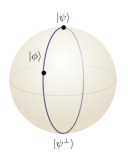
Mathematically, states of the quantum computer are like arrows pointing from the center of the sphere to its surface.
Simple observation "Earth is not flat" leads to quantum algorithms. We will use that when we walk along of the equator, we think we are going straight but eventually we will wrap around it.
Fixing a direction and rotating the arrow, corresponds to a type of of quantum computing operation.
Riemannian geometry underlying quantum algorithms
On a flat surface DOWN-LEFT-UP-RIGHT will return to point of origin.
Riemannian geometry underlying quantum algorithms
On a flat surface DOWN-LEFT-UP-RIGHT will return to point of origin.
On a curved surface SOUTH-WEST-NORTH-EAST will spiral way.
South
West
East
North
Riemannian geometry underlying quantum algorithms
South
West
East
North
My work on double-bracket quantum algorithms shows how to use this spiraling effect to implement non-Euclidean gradient descent in quantum computing.
Regular machine learning fails for quantum computing but our generalization works. The 'failed' machine learning is still key for us - as a warm-start!

(Physical Review Letters '26)
Riemannian geometry underlying quantum algorithms
Riemannian geometry is essential for quantum computation
- The unitary group \(U(d)\) is a Riemannian manifold
- It is an embedded manifold \(U(d) = \{M\in \mathbb C^{d\times d}:~M^{-1}=M^\dagger\}\)
- The tangent space is \(\{W\in \mathbb C^{d\times d}:~W^{\dagger}= -W\} \simeq\{iH \mathrm{~where~} H=H^\dagger\in \mathbb C^{d\times d}\} \)
- The geodesics are matrix exponentials \( \{e^{sW}\}_{s\in\mathbb R} \subset U(d)\) or \( \{e^{isH}\}_{s\in\mathbb R} \subset U(d)\)
- Computing a "gradient" must output an element of the tangent space
\mathbb C^{d\times d}
U(d)
g
W
iH

g^\dagger = -g
e^{s g}
g
g^\dagger = -g
\(\partial_{i,j}\) points to the interior, not tangential
Keep this in mind for later: Unlike in flat space, these 4 steps spiral away from the point of origin
Riemannian geometry is essential for quantum computation
- The unitary group \(U(d)\) is a Riemannian manifold
- The tangent space is \(\{H\in \mathbb C^{d\times d}:~H^{\dagger}= H\} \)
- The geodesics are matrix exponentials \( \{e^{isH}\}_{s\in\mathbb R} \subset U(d)\)
- \(U(d)\) is a curved manifold
e^{is A}e^{is B}e^{-is A}e^{-is B} \neq 1
e^{is A}
e^{isB}
e^{-isB}
e^{-is A}
Operating a quantum computer is all about the group of unitary matrices
\forall A=A^\dagger, B=B^\dagger: ~~M = e^{ [A,B]}\in U(d)
Think of rotations on a sphere
The Lie bracket of two 'velocities' is again a velocity:
Check: \([A,B]^\dagger = (AB- BA)^\dagger = B^\dagger A^\dagger -A^\dagger B^\dagger = -[A,B]\)
M^\dagger = (e^{ [A,B]})^\dagger = e^{ [A,B]^\dagger}=e^{ -[A,B]}=M^{-1}
U(d)
e^{ [A,B]}
\([A,B]^\dagger = -[A,B]\)
Check: \([A,B]^\dagger = -[A,B]\)
U(d) = \{ M\in \mathbb C^{d\times d}: M^{-1} = M^\dagger\}
Operating a quantum computer is all about the group of unitary matrices
\forall A=A^\dagger, B=B^\dagger: ~~M = e^{ [A,B]}\in U(d)
Think of rotations on a sphere
Fact 3: The Lie bracket of two 'velocities' is again a velocity
U(d) = \{ M\in \mathbb C^{d\times d}: M^{-1} = M^\dagger\}
e^{isA}e^{isB}e^{-isA}e^{-isB} = e^{-s^2[A,B]}+O(s^3)
e^{is A}
e^{isB}
e^{-isB}
e^{-is A}
Operating a quantum computer is all about the group of unitary matrices
U(d) = \{ M\in \mathbb C^{d\times d}: M^{-1} = M^\dagger\}
Fact 3: The Lie bracket of two 'velocities' is again a velocity
e^{isA}e^{isB}e^{-isA}e^{-isB} = e^{-s^2[A,B]}+O(s^3)
\forall A=A^\dagger, B=B^\dagger: ~~M = e^{ [A,B]}\in U(d)
The main tool of double-bracket quantum algorithms
e^{is A}
e^{isB}
e^{-isB}
e^{-is A}
E(\psi) = \langle \psi| H | \psi\rangle
| \psi\rangle \mapsto e^{is A}|\psi\rangle
Note that choosing \(A=H\) doesn't change the energy
E(\psi') = \langle \psi| e^{-is H} He^{isH} | \psi\rangle = E(\psi)
Let's find which directions \(A\) are more useful!
\(\partial_{i,j}\) points to the interior, not tangential so which direction is best?
g
W
iH
iA
Same for \(A=\ket{\psi}\bra{\psi}\) because
e^{is \ket\psi\bra\psi} | \psi\rangle = e^{is}\ket\psi
Riemannian gradient: Unique vector \(g\) in the tangent space
such that the directional derivative is a projection onto \(g\)
\nabla_W f(x) = \text{lim}_{s\rightarrow 0}\frac{ f(x+s W) - f(x)}{s} = \langle g, W\rangle
\(\partial_{i,j}\) points to the interior, not tangential so which direction is best?
g
W
iH
iA
Tr(ABC) = Tr(CAB)
\langle g, W\rangle_{\rm{HS}} = \mathrm{Tr}\left(g^\dagger W\right)
(|\psi\rangle\langle \psi|)^\dagger = |\psi\rangle\langle \psi|, H^\dagger = H
We will use very simple ingredients to find \(g\) for \(E(\psi) = \langle \psi| H | \psi\rangle\):
Hilbert-Schmidt scalar product:
Cyclicity of trace:
Tangent space:
Riemannian gradient: Unique vector \(g\) in the tangent space such that the directional derivative is a projection onto \(g\)
\nabla_W f(x) = \text{lim}_{s\rightarrow 0}\frac{ f(x+sW) - f(x)}{s} = \langle g, W\rangle
\nabla_A E(\psi) = \text{lim}_{s\rightarrow 0} \frac{ \langle \psi| e^{-isA}He^{isA}| \psi\rangle- \langle \psi|H | \psi\rangle}{s}
Tr(ABC) = Tr(CAB)\\
\Downarrow \\
Tr(|\psi\rangle\langle \psi| [H,A] ) = Tr([|\psi\rangle\langle \psi|,H]A)
E(\psi) = \langle \psi| H | \psi\rangle
| \psi\rangle \mapsto e^{is A}|\psi\rangle
=\partial_s \langle \psi| e^{-isA}He^{isA}| \psi\rangle_{|s=0}
= iTr\left[|\psi\rangle\langle\psi| [A,H]\right]
\nabla_W f(x) = \langle g, W\rangle
\nabla_A E(\psi) =
\langle- i[|\psi\rangle\langle \psi|,H] , A\rangle_{\rm{HS}}
\\\Downarrow\\
g \equiv -i[|\psi\rangle\langle \psi|,H]
|\psi'\rangle = e^{s[|\psi\rangle\langle \psi|,H]} |\psi\rangle
|\psi\rangle \mapsto e^{isg} |\psi\rangle
|\psi''\rangle = e^{s[|\psi'\rangle\langle \psi'|,H]} |\psi'\rangle
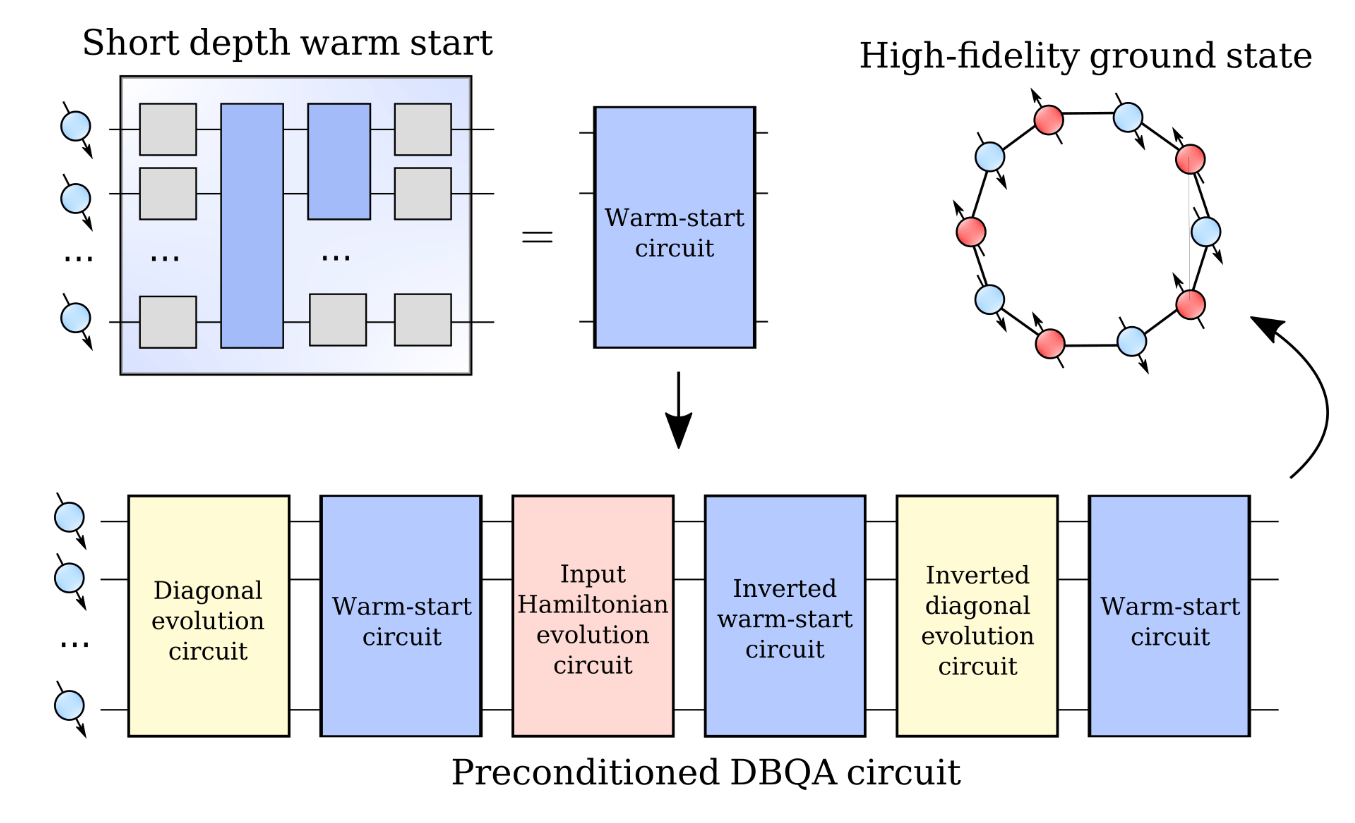
Double-bracket quantum algorithms:
Systematic framework for implementing exponentials of commutators on quantum computers. This uncovered new unitary synthesis formulas.

Riemannian gradient: Unique vector \(g\) in the tangent space such that the directional derivative is a projection onto \(g\)
e^{is A}
e^{isB}
e^{-isB}
e^{-is A}
Double-bracket quantum algorithms
Click these links at slides.com/marekgluza
| Diagonalization | https://arxiv.org/abs/2206.11772 | ||
|---|---|---|---|
| Imaginary-time evolution | https://arxiv.org/abs/2412.04554 | ||
| Quantum signal processing | https://arxiv.org/abs/2504.01077 | ||
| Grover's search | https://arxiv.org/abs/2507.15065 | Approximates ITE |
U^\dagger H U =
\begin{pmatrix}
\lambda_0&&\\
&\lambda_1&\\
&&\ddots
\end{pmatrix}
|\psi(\tau)\rangle = \frac{e^{-\tau H}|\psi\rangle}{\| e^{-\tau H}|\psi\rangle\|}
\frac{ \prod_{k=1}^K(H-z_k I)|\psi\rangle}{\| \prod_{k=1}^K(H-z_k I)|\psi\rangle\|}
\prod_{k=1}^Ke^{i\theta_k|\psi_k\rangle\langle\psi_k|} e^{s_k[|\psi_k\rangle\langle\psi_k|,H]}|\psi\rangle
H' = e^{-s[D,H]}H e^{s[D,H]}
e^{s[|\psi\rangle\langle\psi|,H]}|\psi\rangle +O(\tau^2)
(1-2|\psi\rangle\langle\psi|)\times e^{i t H_f}
e^{s[|\psi\rangle\langle\psi|,H]}|\psi\rangle
Exponentials of commutators solve the unitary synthesis problem in all these cases
Regular gradient descent
Secret sauce when \(x\) is big or \(f(x)\) is costly is the learning rate \(\eta\). Greedy gradient descent will use
\(\eta = \argmin_r f( x_k -r\nabla f(x_k)\))
Next, we do it 'quantumly':
Next, I will show you the optimal line-search solution for linear cost functions like \(C(\ket\psi) = \bra \psi H\ket\psi\)
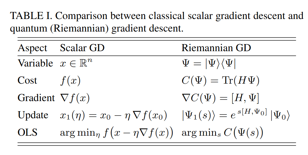
\(s\) is the 'Riemannian' learning rate
\ket{\psi_{k}(s)} = e^{s[\ket{\psi_k}\bra{\psi_k},H]} \ket{\psi_k}
x_{k+1} = x_k -\eta \nabla f(x_k)
\ket{\psi_{k}(s)} = e^{s[\ket{\psi_k}\bra{\psi_k},H]} \ket{\psi_k}
s_k = \argmin_{s\in\mathbb R} \bra{\psi_{k}(s)} H \ket{\psi_{k}(s)}
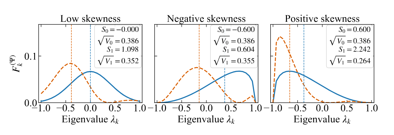
min_{s\in\mathbb R} \bra{\psi_{k}(s)} H \ket{\psi_{k}(s)} = E_k - \sqrt{V_k }\left(\sqrt{1+\tfrac14S_k^2}-\tfrac12{S_k} \right)
S_k ={\bra{\Psi}(H-E_k)^3\ket{\Psi}}/{\sqrt{V_k}^3}
Y. Suzuki

V_k = \bra{\psi_k} H^2\ket{\psi_k}-E_k^2
E_k=\bra{\psi_k} H\ket{\psi_k}
E_{k+1}=E_k -\sqrt{V_k}
Energy filtering in quantum optimization
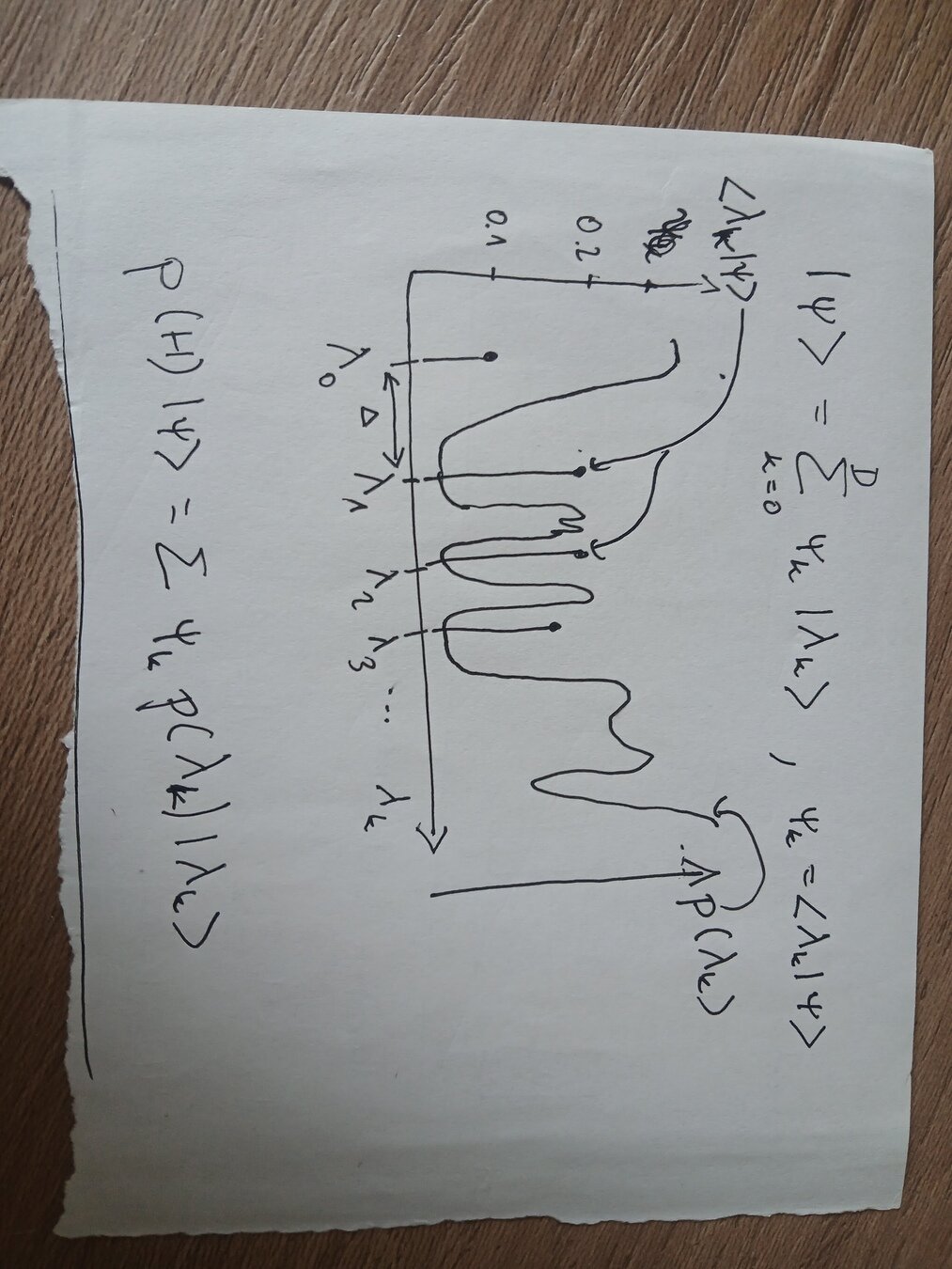
Task: Given Hermitian \(H\), prepare quantum computer in eigenvector \(|\lambda_0\rangle\) with smallest eigenvalue \(\lambda_0\).
\(H = \sum_k \lambda_k |\lambda_k\rangle\langle \lambda_k|\) which is braket notation for: If \(H v_k = \lambda_k v_k\) then \(H= \sum_k \lambda_k v_k^\top v_k\)
After decomposing \(\ket\psi = \sum_k \psi_k \ket{\lambda_k}\) we can filter energy by \(f(H)\ket\psi = \sum_k \psi_k f(\lambda_k) \ket{\lambda_k}\)
Note: We are optimizing \(E(\psi) = \bra\psi H\ket\psi\) and \( \bra{\lambda_0} H\ket{\lambda_0} = \lambda_0\) is the global minimizer
| Imaginary-time evolution |
|
Non-unitary? |
|---|---|---|
| Quantum signal processing | Probabilistic? |
|\psi(\tau)\rangle = \frac{e^{-\tau H}|\psi\rangle}{\| e^{-\tau H}|\psi\rangle\|}
|\psi(z)\rangle = \frac{ p(H)|\psi\rangle}{\| p(H)|\psi\rangle\|}
\(f(\lambda) = e^{-\tau \lambda}\)
\(p(\lambda) = \) Lanczos polynomial
Energy filtering in quantum optimization
Task: Given Hermitian \(H\), prepare quantum computer in eigenvector \(|\lambda_0\rangle\) with smallest eigenvalue \(\lambda_0\).
\(H = \sum_k \lambda_k |\lambda_k\rangle\langle \lambda_k|\) which is braket notation for: If \(H v_k = \lambda_k v_k\) then \(H= \sum_k \lambda_k v_k^\top v_k\)
After decomposing \(\ket\psi = \sum_k \psi_k \ket{\lambda_k}\) we can filter energy by \(f(H)\ket\psi = \sum_k \psi_k f(\lambda_k) \ket{\lambda_k}\)
Note: We are optimizing \(E(\psi) = \bra\psi H\ket\psi\) and \( \bra{\lambda_0} H\ket{\lambda_0} = \lambda_0\) is the global minimizer
f(\tau) = 1-\tau H
E_{k+1}=E_k -\sqrt{V_k}
F_k = |\langle \psi| \lambda_k\rangle|^2
E_k =\sum_k F_k \lambda_k
Energy filtering in quantum optimization
| Imaginary-time evolution |
|
Non-unitary? |
|---|---|---|
| Quantum signal processing | Probabilistic? |
|\psi(\tau)\rangle = \frac{e^{-\tau H}|\psi\rangle}{\| e^{-\tau H}|\psi\rangle\|}
|\psi(z)\rangle = \frac{ p(H)|\psi\rangle}{\| p(H)|\psi\rangle\|}
Task: Given Hermitian \(H\), prepare quantum computer in eigenvector \(|\lambda_0\rangle\) with smallest eigenvalue \(\lambda_0\).
\(f(\lambda) = e^{-\tau \lambda}\)
\(H = \sum_k \lambda_k |\lambda_k\rangle\langle \lambda_k|\) which is braket notation for: If \(H v_k = \lambda_k v_k\) then \(H= \sum_k \lambda_k v_k^\top v_k\)
\(p(\lambda) = \) Lanczos polynomial
After decomposing \(\ket\psi = \sum_k \psi_k \ket{\lambda_k}\) we can filter energy by \(f(H)\ket\psi = \sum_k \psi_k f(\lambda_k) \ket{\lambda_k}\)
Note: We are optimizing \(E(\psi) = \bra\psi H\ket\psi\) and \( \bra{\lambda_0} H\ket{\lambda_0} = \lambda_0\) is the global minimizer
Design choices for optimization
| Diagonalization |
|
Inefficient? |
|---|---|---|
|
Imaginary-time evolution |
Non-unitary? | |
| Quantum signal processing | Probabilistic? |
U^\dagger H U =
\begin{pmatrix}
\lambda_0&&\\
&\lambda_1&\\
&&\ddots
\end{pmatrix}
|\psi(\tau)\rangle = \frac{e^{-\tau H}|\psi\rangle}{\| e^{-\tau H}|\psi\rangle\|}
|\psi(z)\rangle = \frac{ p(H)|\psi\rangle}{\| p(H)|\psi\rangle\|}
\ket{\psi_{k}(s)} = e^{s[\ket{\psi_k}\bra{\psi_k},H]} \ket{\psi_k}
min_{s\in\mathbb R} \bra{\psi_{k}(s)} H \ket{\psi_{k}(s)} = E_k - \sqrt{V_k }\left(\sqrt{1+\tfrac14S_k^2}-\tfrac12{S_k} \right)
S_k =\frac{\bra{\Psi}(H-E_k)^3\ket{\Psi}}{\sqrt{V_k}^3}
V_k = \bra{\psi_k} H^2\ket{\psi_k}-E_k^2
E_k=\bra{\psi_k} H\ket{\psi_k}
s_k = \frac{-\arctan(\frac{2}{S_k})}{2\sqrt{V_k}}
Greedy optimal line-search iteration:
min_{s\in\mathbb R} \bra{\psi_{k}(s)} H \ket{\psi_{k}(s)} = E_k - \sqrt{V_k }\left(\sqrt{1+\tfrac14S_k^2}-\tfrac12{S_k} \right)
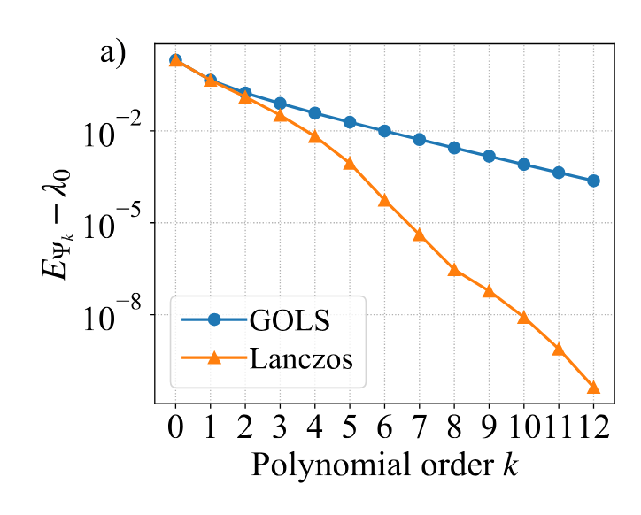
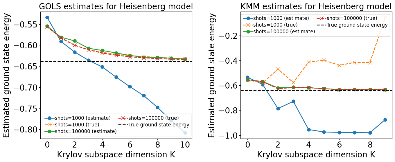
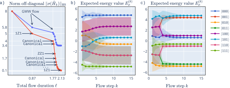
Around step \(k=3\) a global method tempers being greedy.
Then the global method catches up by having a larger \(V_k\) in the subsequent steps.
s_k = \frac{-\arctan(\frac{2}{S_k})}{2\sqrt{V_k}}
Greedy optimal line-search iteration:
min_{s\in\mathbb R} \bra{\psi_{k}(s)} H \ket{\psi_{k}(s)} = E_k - \sqrt{V_k }\left(\sqrt{1+\tfrac14S_k^2}-\tfrac12{S_k} \right)
Geometrically, this means there was a 'ridge' that later eases the climb.
s_k = \frac{-\arctan(\frac{2}{S_k})}{2\sqrt{V_k}}
Greedy optimal line-search iteration:
min_{s\in\mathbb R} \bra{\psi_{k}(s)} H \ket{\psi_{k}(s)} = E_k - \sqrt{V_k }\left(\sqrt{1+\tfrac14S_k^2}-\tfrac12{S_k} \right)
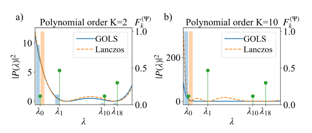
Next, I will tell you that \(k\) steps of Riemannian gradient descent are quantum signal processing by a polynomial of degree \(k\).
This means we can compare to the ideal polynomial the "Lanczos polynomial".
Energy filtering in quantum optimization
| Imaginary-time evolution |
|
Non-unitary? |
|---|---|---|
| Quantum signal processing | Probabilistic? |
|\psi(\tau)\rangle = \frac{e^{-\tau H}|\psi\rangle}{\| e^{-\tau H}|\psi\rangle\|}
|\psi(z)\rangle = \frac{ p(H)|\psi\rangle}{\| p(H)|\psi\rangle\|}
Task: Given Hermitian \(H\), prepare quantum computer in eigenvector \(|\lambda_0\rangle\) with smallest eigenvalue \(\lambda_0\).
\(f(\lambda) = e^{-\tau \lambda}\)
\(H = \sum_k \lambda_k |\lambda_k\rangle\langle \lambda_k|\) which is braket notation for: If \(H v_k = \lambda_k v_k\) then \(H= \sum_k \lambda_k v_k^\top v_k\)
\(p(\lambda) = \) Lanczos polynomial
After decomposing \(\ket\psi = \sum_k \psi_k \ket{\lambda_k}\) we can filter energy by \(f(H)\ket\psi = \sum_k \psi_k f(\lambda_k) \ket{\lambda_k}\)
Note: We are optimizing \(E(\psi) = \bra\psi H\ket\psi\) and \( \bra{\lambda_0} H\ket{\lambda_0} = \lambda_0\) is the global minimizer
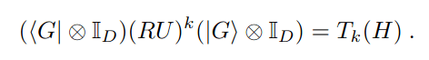
|\psi'\rangle = \frac{P(H) |\psi\rangle}{\|P(H) |\psi\rangle\|} = U_\psi(P) |\psi\rangle
U_\psi(P)
|\phi'\rangle = e^{s[|\phi\rangle\langle\phi|,H]} |\phi\rangle
U_\phi(P) = e^{s[|\phi\rangle\langle\phi|,H]}
We will show that
\(P(H) = 1-\tau_sH\)
Ansatz:
|\psi'\rangle = e^{s[|\psi\rangle\langle \psi|,H]} |\psi\rangle
|\psi'\rangle = \sum_{n=0}^\infty \frac{s^n}{n!} ([|\psi\rangle\langle \psi|,H])^n |\psi\rangle
[|\psi\rangle\langle \psi|,H] |\psi\rangle = |\psi\rangle\langle \psi|H |\psi\rangle - H|\psi\rangle\langle \psi |\psi\rangle
[|\psi\rangle\langle \psi|,H] |\psi\rangle = (E-H) |\psi\rangle
Double-bracket ansatz:
\(n=1\):
([|\psi\rangle\langle \psi|,H])^2 |\psi\rangle = [|\psi\rangle\langle \psi|,H](E-H) |\psi\rangle
([|\psi\rangle\langle \psi|,H])^2 |\psi\rangle = E(E-H) |\psi\rangle - [|\psi\rangle\langle \psi|,H] H |\psi\rangle
= - V|\psi\rangle
([|\psi\rangle\langle \psi|,H])^{2k} |\psi\rangle = (- 1)^k V^k|\psi\rangle
([|\psi\rangle\langle \psi|,H])^{2k+1} |\psi\rangle = (- 1)^k V^k(E-H)|\psi\rangle
[|\psi\rangle\langle \psi|,H] |\psi\rangle = (E-H) |\psi\rangle
\(n=1\):
\(n=2\):
Y. Suzuki
= E^2 |\psi\rangle - EH |\psi\rangle - |\psi\rangle\langle \psi|H^2 |\psi\rangle + E H|\psi\rangle
V =\langle \psi |H^2|\psi\rangle - \langle \psi |H|\psi\rangle^2
([|\psi\rangle\langle \psi|,H])^{2k} |\psi\rangle = (- 1)^k V^k|\psi\rangle
([|\psi\rangle\langle \psi|,H])^{2k+1} |\psi\rangle = (- 1)^k V^k(E-H)|\psi\rangle
This starts looking like quantum signal processing:
Lemma 1. Any linear polynomial with a real root \(P(H) = 1-\tau H\) can be implemented this way.

s_k = \frac{-\arctan(\frac{2}{S_k})}{2\sqrt{V_k}}
Greedy optimal line-search iteration:
min_{s\in\mathbb R} \bra{\psi_{k}(s)} H \ket{\psi_{k}(s)} = E_k - \sqrt{V_k }\left(\sqrt{1+\tfrac14S_k^2}-\tfrac12{S_k} \right)
There is a very nice method for finding the Lanczos polynomial from block-encodings
Being greedy makes you globally slower
Being greedy makes you more stable under noise!
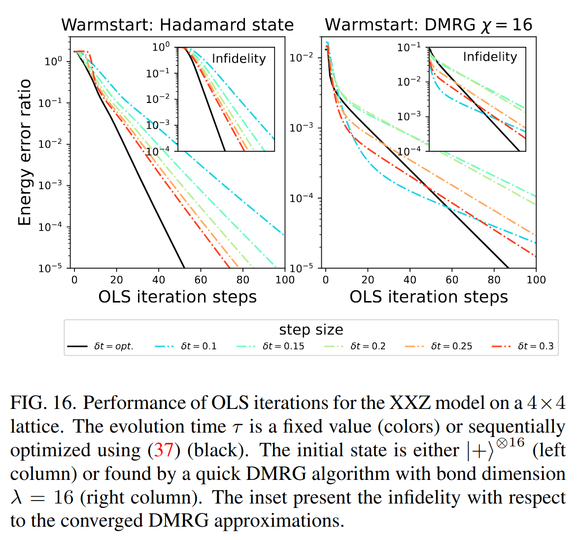
Full compilation in Qrisp of GOLS and KMM
Checking GOLS with MPS
New solver for Krylov spaces:
Iterating OLS to converge to Lanczos by removing random roots and finding new ones
E_{k+1} \ge E_k - \sqrt{V_k }\left(\sqrt{1+\tfrac14S_k^2}-\tfrac12{S_k} \right)
On Arxiv soon-ish
Full compilation in Qrisp of GOLS and KMM
Checking GOLS with MPS
New solver for Krylov spaces:
Iterating OLS to converge to Lanczos by removing random roots and finding new ones
E_{k+1} \ge E_k - \sqrt{V_k }\left(\sqrt{1+\tfrac14S_k^2}-\tfrac12{S_k} \right)
On Arxiv soon-ish
4 stages of creating quantum algorithms
1. Design choice:
How to go about it?
|\psi(\tau)\rangle = \frac{e^{-\tau H}|\psi\rangle}{\| e^{-\tau H}|\psi\rangle\|}
2. Unitary synthesis:
How to do it?
3. Circuit compilation:
What gates to do?
0. Problem choice:
What challenge to take up?
Double-bracket quantum algorithms:
Systematic framework for unitary synthesis
4 stages of creating quantum algorithms
1. Design choice:
How to go about it?
|\psi(\tau)\rangle = \frac{e^{-\tau H}|\psi\rangle}{\| e^{-\tau H}|\psi\rangle\|}
3. Circuit compilation:
What gates to do?
0. Problem choice:
What challenge to take up?
2. Unitary synthesis:
How to do it?
Double-bracket quantum algorithms:
Systematic framework for unitary synthesis
4 stages of creating quantum algorithms
E(\psi) = \langle \psi| H | \psi\rangle
4 stages of creating quantum algorithms
1. Design choice:
How to go about it?
|\psi(\tau)\rangle = \frac{e^{-\tau H}|\psi\rangle}{\| e^{-\tau H}|\psi\rangle\|}
3. Circuit compilation:
What gates to do?
|\psi(\tau)\rangle = \frac{e^{-\tau H}|\psi\rangle}{\| e^{-\tau H}|\psi\rangle\|}
0. Problem choice:
What challenge to take up?
2. Unitary synthesis:
How to do it?
4 stages of creating quantum algorithms
Imaginary-time evolution
\ket\psi\rightarrow |\psi(\tau)\rangle
H = \sum_{k=1}^{D} \lambda_k \ket{\lambda_k}\bra{\lambda_k}
e^{-\tau H}|\psi\rangle = \langle\lambda_0|\psi\rangle \ket{\lambda_0} +\sum_{k=1}^{D} e^{-\tau\lambda_k} \langle\lambda_k|\psi\rangle \ket{\lambda_k}
|\psi\rangle = \langle\lambda_0|\psi\rangle \ket{\lambda_0} +\sum_{k=1}^{D} \langle\lambda_k|\psi\rangle \ket{\lambda_k}
\lim_{\tau\rightarrow \infty}\ket{\psi(\tau)} = \ket{\lambda_0}
4 stages of creating quantum algorithms
1. Design choice:
How to go about it?
|\psi(\tau)\rangle = \frac{e^{-\tau H}|\psi\rangle}{\| e^{-\tau H}|\psi\rangle\|}
3. Circuit compilation:
What gates to do?
|\psi(\tau)\rangle = \frac{e^{-\tau H}|\psi\rangle}{\| e^{-\tau H}|\psi\rangle\|}
0. Problem choice:
What challenge to take up?
2. Unitary synthesis:
How to do it?
|\psi(\tau)\rangle = \frac{e^{-\tau H}|\psi\rangle}{\| e^{-\tau H}|\psi\rangle\|}
= e^{\tau[|\psi\rangle\langle\psi|,H]}|\psi\rangle +O(\tau^2)
4 stages of creating quantum algorithms
4 stages of creating quantum algorithms
1. Design choice:
How to go about it?
|\psi(\tau)\rangle = \frac{e^{-\tau H}|\psi\rangle}{\| e^{-\tau H}|\psi\rangle\|}
3. Circuit compilation:
What gates to do?
0. Problem choice:
What challenge to take up?
2. Unitary synthesis:
How to do it?
Double-bracket quantum algorithms:
Systematic framework for unitary synthesis
4 stages of creating quantum algorithms
E(\psi) = \langle \psi| H | \psi\rangle
Operating a quantum computer is all about the group of unitary matrices
\forall A=A^\dagger, B=B^\dagger: ~~M = e^{ [A,B]}\in U(d)
Fact 3: The Lie bracket of two 'velocities' is again a velocity
U(d) = \{ M\in \mathbb C^{d\times d}: M^{-1} = M^\dagger\}
e^{isA}e^{isB}e^{-isA}e^{-isB} = e^{-s^2[A,B]}+O(s^3)
e^{is A}
e^{isB}
e^{-isB}
e^{-is A}
Operating a quantum computer is all about the group of unitary matrices
U(d) = \{ M\in \mathbb C^{d\times d}: M^{-1} = M^\dagger\}
Fact 3: The Lie bracket of two 'velocities' is again a velocity
e^{isA}e^{isB}e^{-isA}e^{-isB} = e^{-s^2[A,B]}+O(s^3)
\forall A=A^\dagger, B=B^\dagger: ~~M = e^{ [A,B]}\in U(d)
The main tool of double-bracket quantum algorithms
e^{is A}
e^{isB}
e^{-isB}
e^{-is A}
4 stages of creating quantum algorithms
1. Design choice:
How to go about it?
|\psi(\tau)\rangle = \frac{e^{-\tau H}|\psi\rangle}{\| e^{-\tau H}|\psi\rangle\|}
3. Circuit compilation:
What gates to do?
0. Problem choice:
What challenge to take up?
2. Unitary synthesis:
How to do it?
Double-bracket quantum algorithms:
Systematic framework for unitary synthesis
4 stages of creating quantum algorithms
|\psi(\tau)\rangle = \frac{e^{-\tau H}|\psi\rangle}{\| e^{-\tau H}|\psi\rangle\|}
E(\psi) = \langle \psi| H | \psi\rangle
e^{s[|\psi\rangle\langle \psi|,H]} |\psi\rangle
4 stages of creating quantum algorithms
\frac{e^{-\tau H}|\psi\rangle}{\| e^{-\tau H}|\psi\rangle\|}
= e^{\tau[|\psi\rangle\langle\psi|,H]}|\psi\rangle +O(\tau^2)
Product formula approximation:
\(e^{\tau[|\psi\rangle\langle\psi|,H]} = e^{i\sqrt{\tau}H}e^{i\sqrt{\tau}|\psi\rangle\langle\psi|}e^{-i\sqrt{\tau}H}e^{-i\sqrt{\tau}|\psi\rangle\langle\psi|} + O(\tau^{3/2})\)
4 stages of creating quantum algorithms
2. Unitary synthesis:
How to do it?
1. Design choice:
How to go about it?
|\psi(\tau)\rangle = \frac{e^{-\tau H}|\psi\rangle}{\| e^{-\tau H}|\psi\rangle\|}
3. Circuit compilation:
What gates to do?
|\psi(\tau)\rangle = \frac{e^{-\tau H}|\psi\rangle}{\| e^{-\tau H}|\psi\rangle\|}
0. Problem choice:
What challenge to take up?
= e^{i\sqrt{\tau}H}e^{i\sqrt{\tau}|\psi\rangle\langle\psi|}e^{i\sqrt{\tau}H}|\psi\rangle + O(\tau^{3/2})
3. Circuit compilation:
What gates to do?
Product formula approximation:
\(e^{\tau[|\psi\rangle\langle\psi|,H]} = e^{i\sqrt{\tau}H}e^{i\sqrt{\tau}|\psi\rangle\langle\psi|}e^{-i\sqrt{\tau}H}e^{-i\sqrt{\tau}|\psi\rangle\langle\psi|} + O(\tau^{3/2})\)
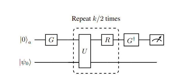
Quantum algorithm DB-QITE - iterate recursively:
- Define \(|{\psi_k}\rangle = U_k |0\rangle\)
- Use \(e^{is |\psi_k\rangle\langle\psi_k|} = U_ke^{is |0\rangle\langle0|}U_k^\dagger \)
- Recursively iterate \( U_{k+1} = e^{is H} U_k e^{is |0\rangle\langle 0|} U_k^\dagger e^{-is H} U_k\)
3 stages of creating quantum algorithms
1. Design choice:
How to go about it?
3. Circuit compilation:
What gates to do?
|\psi(\tau)\rangle = \frac{e^{-\tau H}|\psi\rangle}{\| e^{-\tau H}|\psi\rangle\|}
0. Problem choice:
What challenge to take up?
e^{itH}\\
e^{it|\psi\rangle\langle\psi|}
4 stages of creating quantum algorithms
2. Unitary synthesis:
How to do it?
(PRL '26)
3. Circuit compilation:
What gates to do?
Product formula approximation:
\(e^{\tau[|\psi\rangle\langle\psi|,H]} = e^{i\sqrt{\tau}H}e^{i\sqrt{\tau}|\psi\rangle\langle\psi|}e^{-i\sqrt{\tau}H}e^{-i\sqrt{\tau}|\psi\rangle\langle\psi|} + O(\tau^{3/2})\)
Quantum algorithm DB-QITE - iterate recursively:
- Define \(|{\psi_k}\rangle = U_k |0\rangle\)
- Use \(e^{is |\psi_k\rangle\langle\psi_k|} = U_ke^{is |0\rangle\langle0|}U_k^\dagger \)
- Recursively iterate \( U_{k+1} = e^{is H} U_k e^{is |0\rangle\langle 0|} U_k^\dagger e^{-is H} U_k\)
3 stages of creating quantum algorithms
1. Design choice:
How to go about it?
3. Circuit compilation:
What gates to do?
|\psi(\tau)\rangle = \frac{e^{-\tau H}|\psi\rangle}{\| e^{-\tau H}|\psi\rangle\|}
0. Problem choice:
What challenge to take up?
e^{itH}\\
e^{it|\psi\rangle\langle\psi|}
4 stages of creating quantum algorithms
2. Unitary synthesis:
How to do it?
(accepted at PRL)
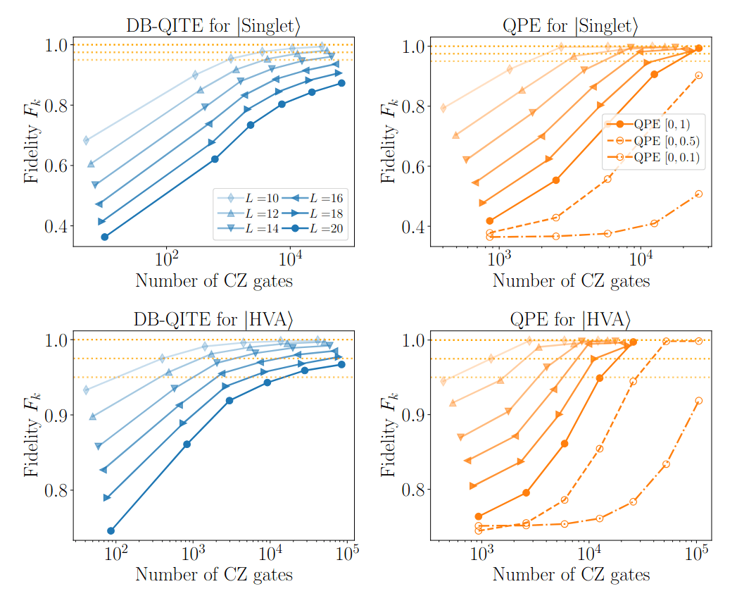
Numerical results for DB-QITE:
DB-QITE:
- Define \(|{\psi_k}\rangle = U_k |0\rangle\)
- Recursively iterate \( U_{k+1} = e^{is H} U_k e^{is |0\rangle\langle 0|} U_k^\dagger e^{-is H} U_k\)
Then:


Quantinuum
(accepted at PRL)
Quantum computing: What do we really have?
Yes. But: Is it really enough?
Quantum winter
Quantum computers
Useful tasks?
If for
No
Then
BUT!

Quantum winter
Quantum computers
Useful tasks!
If for
No
Then
Material science?


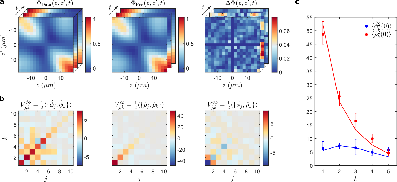
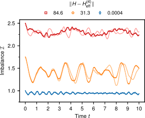
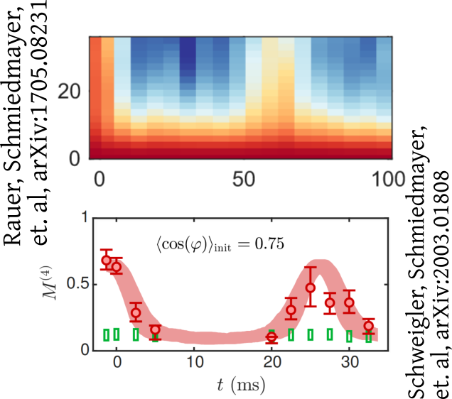
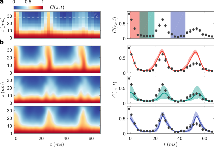
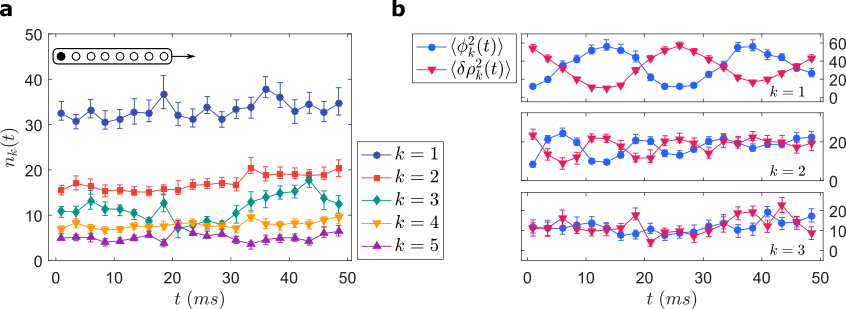
\langle\hat \phi_k^2(t)\rangle= \cos^2(\omega_k t) \langle \phi_k^2(0)\rangle \\
\quad\quad\quad\quad\quad+\sin^2(\omega_k t) \langle \delta\hat \rho_k^2(0)\rangle

\delta \hat\rho
\langle\hat \phi^2(t)\rangle
\langle\delta\hat \rho^2(0)\rangle =0?
\langle \hat \phi^2(0)\rangle
\hat \phi
Ask me anytime:
[4,8]
[1]

[3]
[2]
[5]
[13]

[6]

[9]
[11,16]
[12]
[7, 14, 15, 17]
[10]

0
0
0
0
C
Fidelity witnesses
Tomography optical lattices
Tomography phonons
Proving statistical mechanics
Quantum simulating DSF
Holography in tensor networks
PEPS contraction average #P-hard
Quantum field machine
MBL l-bits
Gaussian quantum simulators

How?
Ultra-cold 1d gases
Inside: atoms
Outside: wavepackets
hydrodynamics
Energy of phonons


E
E
E
E

\hat H_\text{TLL} = \int \text{d}z\left[ \frac{\hbar^2n_{GP}}{2m}\partial_z\hat\varphi^2+g\delta\hat\varrho^2\right]
\delta\varrho
\partial_z\varphi
\partial_z\varphi
\ll
\delta\varrho
\ll
Tomonaga-Luttinger liquid
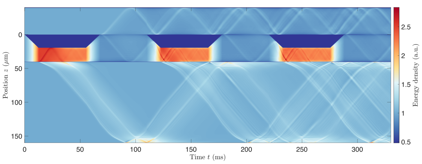
Quantum field refrigerators in the TLL model:
System
Piston
Bath
Bath with excitations
System cooled down
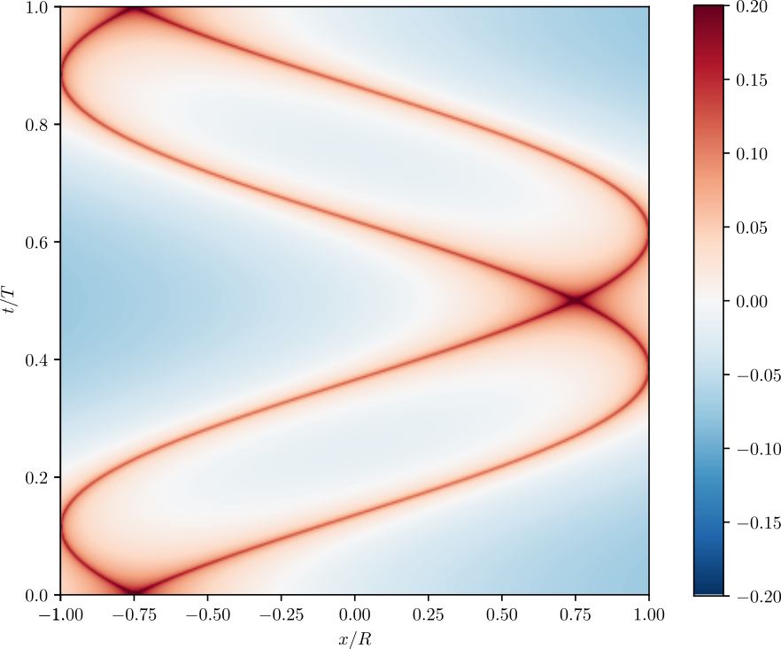
Breaking of the Huygens-Fresnel principle
in the inhomogenous TLL model:
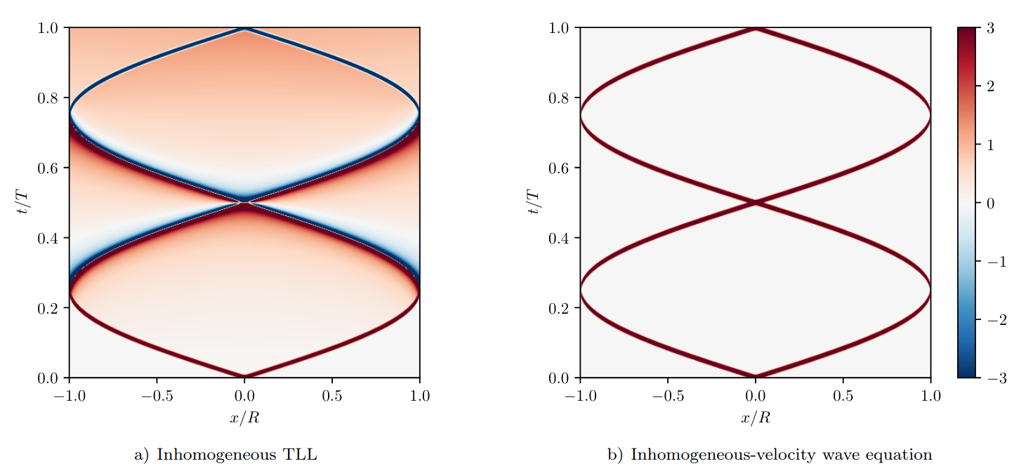
Why?
Why develop continuous field
quantum simulators?
- Representation theory: Quantum information?
- Continuum limits: BQP and QMA or more?
- Are nanowires computationally hard to simulate?
What do we know is difficult?


SM
Fundamental
Universal
Effective
Why develop continuous field
quantum simulators?
- Representation theory: Quantum information?
- Continuum limits: BQP and QMA or more?
- Are nanowires computationally hard to simulate?
What do we know is difficult?
SM
Fundamental
Universal
Effective
Non-thermal
steady states
Sine-Gordon
thermal states
Atomtronics
Generalized hydrodynamics
Recurrences
Some highlights:
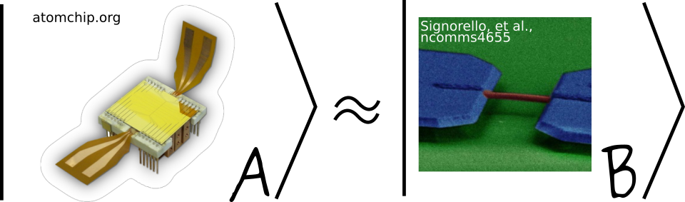
Interferometry measures velocities

van Nieuwkerk, Schmiedmayer, Essler, arXiv:1806.02626
Schumm, Schmiedmayer, Kruger, et al., arXiv:quant-ph/0507047
\partial_z\hat \varphi(z) \approx\frac{\hat \varphi(z)-\hat \varphi(z+\Delta z)}{\Delta z}
\partial_z\hat \varphi(z) \approx\frac{\Delta\hat\varphi(z)}{\Delta z}
\Delta z
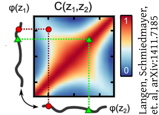
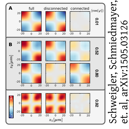
Tomography
Tomography for phonons
\hat H_\text{TLL} = \int \text{d}z\left[ \frac{\hbar^2n_{GP}}{2m}\partial_z\hat\varphi^2+g\delta\hat\varrho^2\right]
\hat H_\text{TLL} = \sum_{k>0} \frac {\hbar \omega_k}2 (\phi_k^2+\delta\hat\rho_k^2) + g\hat\rho_0^2
\langle\hat \phi_k^2(t)\rangle= \cos^2(\omega_k t) \langle \phi_k^2(0)\rangle \\
\quad\quad\quad\quad\quad+\sin^2(\omega_k t) \langle \delta\hat \rho_k^2(0)\rangle
\delta \hat\rho
\langle\hat \phi^2(t)\rangle
\langle\delta\hat \rho^2(0)\rangle =0?
\langle \hat \phi^2(0)\rangle
\hat \phi
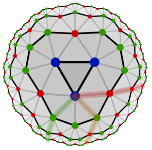
What are eigenmodes?
\hat H_\text{TLL} = \int \text{d}z\left[ \frac{\hbar^2n_{GP}}{2m}\partial_z\hat\varphi^2+g\delta\hat\varrho^2\right]
\hat H_\text{TLL} = \sum_{k>0} \frac {\hbar \omega_k}2 (\phi_k^2+\delta\hat\rho_k^2) + g\hat\rho_0^2
\hat \phi_k = \int_0^L dz \cos(\pi k z/L)\hat \varphi(z)
\int_0^L dz \cos(\pi k z/L)\cos(\pi k'z/L) = \delta_{k,k'}
Transmutation
\langle\hat \phi_k^2(t)\rangle= \cos^2(\omega_k t) \langle \hat\phi_k^2(0)\rangle +\sin^2(\omega_k t) \langle \delta\hat \rho_k^2(0)\rangle
\langle\hat \phi_k^2(t)\rangle= \langle \hat\phi_k^2(0)\rangle
\langle\hat \phi_k^2(t)\rangle= \langle \delta\hat \rho_k^2(0)\rangle
t=0:
t=\frac{\pi}{2\omega_k}:
\delta \hat\rho
\langle\hat \phi^2(t)\rangle
\langle\delta\hat \rho^2(0)\rangle =0?
\langle \hat \phi^2(0)\rangle
\hat \phi
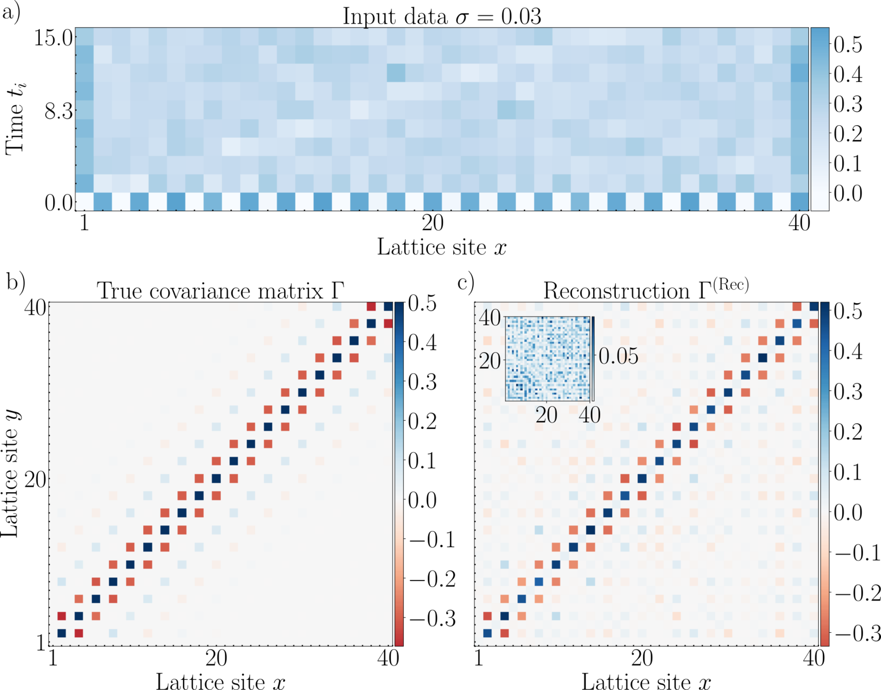
Tomography
A_{1,2}= \sin^2(\omega_k t_1 )
A_{1,1}= \cos^2(\omega_k t_1)
\langle\hat \phi_k^2(t)\rangle= \cos^2(\omega_k t) \langle \hat\phi_k^2(0)\rangle+ \sin^2(\omega_k t) \langle \delta\hat \rho_k^2(0)\rangle
A_{3,2}= \sin^2(\omega_k t_3 )
A_{3,1}= \cos^2(\omega_k t_3)
A_{2,2}= \sin^2(\omega_k t_2 )
A_{2,1}= \cos^2(\omega_k t_2)
A
\begin{pmatrix} \langle \hat\phi_k^2(0)\rangle \\\langle \delta\hat \rho_k^2(0)\rangle
\end{pmatrix}
=\begin{pmatrix} \langle \hat\phi_k^2(t_1)\rangle \\\langle \hat\phi_k^2(t_2)\rangle \\\langle \hat\phi_k^2(t_3)\rangle \end{pmatrix}
\|Aq - d\| = \text{min}
(This formalism: Tomography for many modes)

Tomography Klein-Gordon thermal state after quench
\hat H_\text{KG}=\hat H_\text{TLL}+J\int \mathrm{d}z \,n_{GP} \hat \varphi^2
Extracting physical properties
Extracting physical properties
Extracting physical properties
Tomography for optical lattices

SQST 2026
By Marek Gluza


