Quantum algorithms for optimisation derived from the non-Euclidean geometry of quantum computing operations
Marek Gluza
NTU Singapore
Scan QR code or go to slides.com/marekgluza

What is a quantum computer?
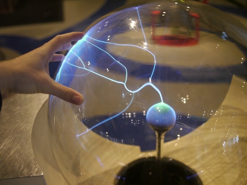
It is a quantum system e.g. ionized atom, loop of a superconductor
It is modeled by a finite dimensional vector space \(\mathcal V = \mathbb C^d\)
It is modular: We can add more of its components and make \(d\) grow
It is programmable: There are ways (quantum gates) to change its states in a reproducible and reversible manner
It is universal: Composing sufficiently many of the programmable operations allows to approximate any \(v = |v\rangle \in \mathcal V\)
We take more qubits
Apply patterned EM radiation
Reproducible: Use FPGA
Reversible: Physics challenge; keep cold
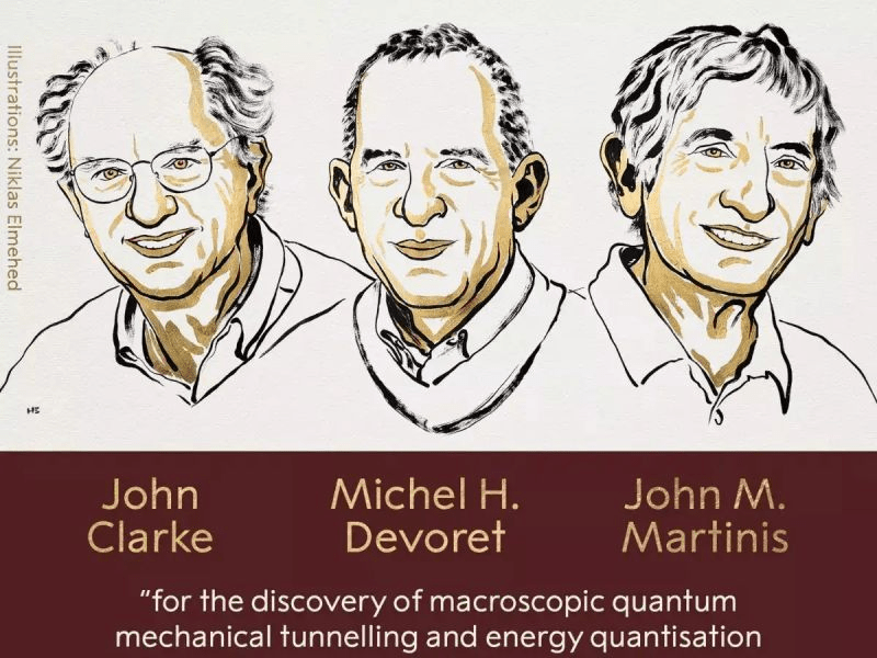
Physics papers from the 90's
|
|
|
|---|---|
|
|
|
|
|
|
|
|
|
|
|
We can make it!
We take \(n\) qubits then \(\mathcal V = (\mathbb C^2)^{\otimes n}\) and \(d=2^n\)
What is a quantum computer?
A quantum computer is an experimental setup A which includes a quantum system B and that setup A allows to manipulate the quantum state of B.
This is modeled by mulitplying unitary matrices to vectors from a finite-dimensional vector space.
Types of quantum computers:
- A) Superconducting loops
- B) Ionized atoms
- C) Neutral atoms
- D) Others
Companies:
- A) Google, IQM, IBM, Rigetti
- B) Quantinuum, IonQ
- C) Quera, Atom Computing, Pasqal
- D) Alice&Bob, Qolab, Normal Computing, Psi-Quantum,
Zapata
Currently 80 companies listed here:
https://thequantuminsider.com/2025/09/23/top-quantum-computing-companies/
What are quantum algorithms?
We model quantum computing operations by mulitplying unitary matrices to vectors from a finite-dimensional vector space:
- States of the quantum computer are vectors.
- Operations on the quantum computer rotate these vectors.
- Two consecutive rotations are a rotation.
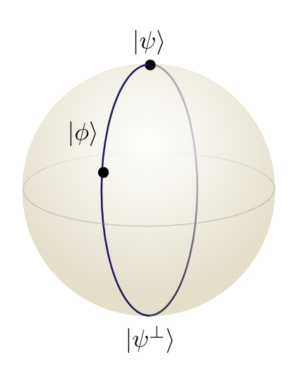
- The space of all rotations generalizes the geometry of the sphere.
- Straight lines in the space of rotations are those which don't change their direction.
- Going SOUTH-WEST-NORTH-EAST in the space of all rotations spirals away from the point of origin.
- Repeating two directions sufficiently many times will bring you eventually everywhere.
Braket notation
|\psi\rangle = a | 0 \rangle + b | 1\rangle
\langle \vec v,\vec w\rangle \leftrightarrow \langle \phi|\psi\rangle
1 qubit:
*The biography of the physicist who proposed it is literally called "The strangest man"

\mathcal V = \mathbb C^2 = \mathrm{span}_{\mathbb C}\{ e_1, e_2\}
| 0 \rangle :=e_1, | 1\rangle :=e_2
v \in \mathcal V \leftrightarrow |v\rangle = v_0 | 0 \rangle + v_1 | 1\rangle
\langle \vec v,A \vec v\rangle \leftrightarrow \langle \psi|H|\psi\rangle
A \vec v \leftrightarrow H|\psi\rangle
*Dirac was one of the smartest quantum physicist in history
\vec v^\dagger \in \mathcal V^* \leftrightarrow \langle \psi|
"ket"
"bra"
"bracket"
"quantum superposition"
What is a universal quantum computer?
|\psi\rangle = a | 0 \rangle + b | 1\rangle
|\psi\rangle = a | 00 \rangle + b | 10\rangle+c | 01 \rangle + b | 11\rangle
|\psi\rangle = a | 000 \rangle + b | 100\rangle+c | 010 \rangle + d | 100\rangle+
e | 011 \rangle + f | 101\rangle+g | 110 \rangle +h | 111\rangle
|\psi\rangle = a | 0000 \rangle + b | 1000\rangle+c | 0100 \rangle + d | 1000\rangle+
e | 0011 \rangle + f | 0101\rangle+g | 1010 \rangle +h | 1100\rangle + \ldots
1 qubit
2 qubits
3 qubits
4 qubits
|\psi\rangle = U |00\ldots0\rangle \Rightarrow U \approx U_c
it can approximate any state preparation via circuits
It is a machine for realizing such linear combinations in nature
0
0
0
0
C
Operating a quantum computer is all about the group of unitary matrices
M,M' \in U(d) \Rightarrow (M M')(MM')^\dagger = M (M'M'^\dagger) M^\dagger
= M M^\dagger = I
\Rightarrow (M M')\in U(d)
\ket{\psi'} = M \ket\psi \Rightarrow \ket{\psi''} = M'\ket{\psi'} = M'M \ket\psi
Think of rotations on a sphere
U(d) = \{ M\in \mathbb C^{d\times d}: M^{-1} = M^\dagger\}
|\psi'\rangle
|\psi\rangle
|\psi''\rangle
|\psi\rangle = U |00\ldots0\rangle
What are quantum algorithms?
We model quantum computing operations by mulitplying unitary matrices to vectors from a finite-dimensional vector space:
- States of the quantum computer are vectors.
- Operations on the quantum computer rotate these vectors.
- Two consecutive rotations are a rotation.
- The space of all rotations generalizes the geometry of the sphere.
- Straight lines in the space of rotations are those which don't change their direction.
- Going SOUTH-WEST-NORTH-EAST in the space of all rotations spirals away from the point of origin.
- Repeating two directions sufficiently many times will bring you eventually everywhere.
Riemannian geometry is essential for quantum computation
- The unitary group \(U(d)\) is a Riemannian manifold
- It is an embedded manifold \(U(d) = \{M\in \mathbb C^{d\times d}:~M^{-1}=M^\dagger\}\)
- The tangent space is \(\{W\in \mathbb C^{d\times d}:~W^{\dagger}= -W\} \simeq\{iH \mathrm{~where~} H=H^\dagger\in \mathbb C^{d\times d}\} \)
- The geodesics are matrix exponentials \( \{e^{sW}\}_{s\in\mathbb R} \subset U(d)\) or \( \{e^{isH}\}_{s\in\mathbb R} \subset U(d)\)
- Computing a "gradient" must output an element of the tangent space
\mathbb C^{d\times d}
U(d)
g
W
iH

g^\dagger = -g
e^{s g}
g
g^\dagger = -g
\(\partial_{i,j}\) points to the interior, not tangential
To go straight to New York, follow the equator. Don't drill a tunnel to literally go straight.
Unlike in flat space, going SOUTH-WEST-NORTH-EAST in the space of all rotations spirals away from the point of origin.
Riemannian geometry is essential for quantum computation
- The unitary group \(U(d)\) is a Riemannian manifold
- The tangent space is \(\{H\in \mathbb C^{d\times d}:~H^{\dagger}= H\} \)
- The geodesics are matrix exponentials \( \{e^{isH}\}_{s\in\mathbb R} \subset U(d)\)
- \(U(d)\) is a curved manifold
e^{is A}e^{is B}e^{-is A}e^{-is B} \neq 1
e^{is A}
e^{isB}
e^{-isB}
e^{-is A}
Operating a quantum computer is all about the group of unitary matrices
\exist G_1,G_2,\ldots G_K \in U(d) \mathrm{~such~that}
Think of rotations on a sphere
Universal quantum computation means: Composing sufficiently many basic unitary matrices (elementary quantum gates \(G_1,G_2,\ldots, G_K\)) can approximate any other 'larger' unitary.
(finding these sequences = task of unitary synthesis)
U(d) = \{ M\in \mathbb C^{d\times d}: M^{-1} = M^\dagger\}
\forall M \in U(d)~\exist \mathrm{sequence~s.t.} ~M\approx G_1 G_5G_6G_1 G_K G_1 G_2\ldots
4 stages of creating quantum algorithms
1. Design choice:
How to go about it?
|\psi(\tau)\rangle = \frac{e^{-\tau H}|\psi\rangle}{\| e^{-\tau H}|\psi\rangle\|}
2. Unitary synthesis:
How to do it?

3. Circuit compilation:
What gates to do?
0. Problem choice:
What challenge to take up?
Double-bracket quantum algorithms:
Systematic framework for unitary synthesis
Quantum computing cannot be useful if
- The problem can be solved quickly on classical computers
- Solving the problem isn't important
- Solving the problem is too hard for the quantum computer
Classical computation
Key question in current quantum computation:
Find an important problem which is difficult yet doable
Millenials
What challenge to take up?
Quantum computing cannot be useful if
- The problem can be solved quickly on classical computers
- Solving the problem isn't important
- Solving the problem is too hard for the quantum computer
Key question in current quantum computation:
Find an important problem which is difficult yet doable
What challenge to take up?
Materials science?
Why materials science? Imagine improving photovoltaics by 1%.
What needs to be done? Perform \(\bra\psi H\ket\psi\) optimization.
How? Quantum circuit synthesis.
0. Problem choice:
What challenge to take up?
Materials science?
Quantum computing cannot be useful if
- The problem can be solved quickly on classical computers
- Solving the problem isn't important
- Solving the problem is too hard for the quantum computer
Why materials science? Imagine improving photovoltaics by 1%.
What needs to be done? Perform \(\bra\psi H\ket\psi\) optimization.
How? Quantum circuit synthesis.
Non-Euclidean geometry leads to quantum algorithms
Next: How to get $$ from a quantum computer?
We need to optimize among all operations of the quantum computer to get a low-energy state
(Non-Euclidean optimization)
E(\psi) = \langle \psi| H | \psi\rangle
4 stages of creating quantum algorithms
1. Design choice:
How to go about it?
|\psi(\tau)\rangle = \frac{e^{-\tau H}|\psi\rangle}{\| e^{-\tau H}|\psi\rangle\|}
3. Circuit compilation:
What gates to do?
0. Problem choice:
What challenge to take up?
2. Unitary synthesis:
How to do it?
Double-bracket quantum algorithms:
Systematic framework for unitary synthesis
4 stages of creating quantum algorithms
E(\psi) = \langle \psi| H | \psi\rangle
4 stages of creating quantum algorithms
1. Design choice:
How to go about it?
|\psi(\tau)\rangle = \frac{e^{-\tau H}|\psi\rangle}{\| e^{-\tau H}|\psi\rangle\|}
3. Circuit compilation:
What gates to do?
|\psi(\tau)\rangle = \frac{e^{-\tau H}|\psi\rangle}{\| e^{-\tau H}|\psi\rangle\|}
0. Problem choice:
What challenge to take up?
2. Unitary synthesis:
How to do it?
4 stages of creating quantum algorithms
Imaginary-time evolution
\ket\psi\rightarrow |\psi(\tau)\rangle
H = \sum_{k=1}^{D} \lambda_k \ket{\lambda_k}\bra{\lambda_k}
e^{-\tau H}|\psi\rangle = \langle\lambda_0|\psi\rangle \ket{\lambda_0} +\sum_{k=1}^{D} e^{-\tau\lambda_k} \langle\lambda_k|\psi\rangle \ket{\lambda_k}
|\psi\rangle = \langle\lambda_0|\psi\rangle \ket{\lambda_0} +\sum_{k=1}^{D} \langle\lambda_k|\psi\rangle \ket{\lambda_k}
\lim_{\tau\rightarrow \infty}\ket{\psi(\tau)} = \ket{\lambda_0}
4 stages of creating quantum algorithms
1. Design choice:
How to go about it?
|\psi(\tau)\rangle = \frac{e^{-\tau H}|\psi\rangle}{\| e^{-\tau H}|\psi\rangle\|}
3. Circuit compilation:
What gates to do?
|\psi(\tau)\rangle = \frac{e^{-\tau H}|\psi\rangle}{\| e^{-\tau H}|\psi\rangle\|}
0. Problem choice:
What challenge to take up?
2. Unitary synthesis:
How to do it?
|\psi(\tau)\rangle = \frac{e^{-\tau H}|\psi\rangle}{\| e^{-\tau H}|\psi\rangle\|}
= e^{\tau[|\psi\rangle\langle\psi|,H]}|\psi\rangle +O(\tau^2)
4 stages of creating quantum algorithms
4 stages of creating quantum algorithms
1. Design choice:
How to go about it?
|\psi(\tau)\rangle = \frac{e^{-\tau H}|\psi\rangle}{\| e^{-\tau H}|\psi\rangle\|}
3. Circuit compilation:
What gates to do?
0. Problem choice:
What challenge to take up?
2. Unitary synthesis:
How to do it?
Double-bracket quantum algorithms:
Systematic framework for unitary synthesis
4 stages of creating quantum algorithms
E(\psi) = \langle \psi| H | \psi\rangle
Operating a quantum computer is all about the group of unitary matrices
\forall A=A^\dagger, B=B^\dagger: ~~M = e^{ [A,B]}\in U(d)
Think of rotations on a sphere
The Lie bracket of two 'velocities' is again a velocity:
Check: \([A,B]^\dagger = (AB- BA)^\dagger = B^\dagger A^\dagger -A^\dagger B^\dagger = -[A,B]\)
M^\dagger = (e^{ [A,B]})^\dagger = e^{ [A,B]^\dagger}=e^{ -[A,B]}=M^{-1}
U(d)
e^{ [A,B]}
\([A,B]^\dagger = -[A,B]\)
Check: \([A,B]^\dagger = -[A,B]\)
U(d) = \{ M\in \mathbb C^{d\times d}: M^{-1} = M^\dagger\}
Operating a quantum computer is all about the group of unitary matrices
\forall A=A^\dagger, B=B^\dagger: ~~M = e^{ [A,B]}\in U(d)
Think of rotations on a sphere
Fact 3: The Lie bracket of two 'velocities' is again a velocity
U(d) = \{ M\in \mathbb C^{d\times d}: M^{-1} = M^\dagger\}
e^{isA}e^{isB}e^{-isA}e^{-isB} = e^{-s^2[A,B]}+O(s^3)
e^{is A}
e^{isB}
e^{-isB}
e^{-is A}
Operating a quantum computer is all about the group of unitary matrices
U(d) = \{ M\in \mathbb C^{d\times d}: M^{-1} = M^\dagger\}
Think of rotations on a sphere
Fact 3: The Lie bracket of two 'velocities' is again a velocity
My quantum algorithms use such unitary matrices - they are implementing Riemannian gradient descent
e^{isA}e^{isB}e^{-isA}e^{-isB} = e^{-s^2[A,B]}+O(s^3)
\forall A=A^\dagger, B=B^\dagger: ~~M = e^{ [A,B]}\in U(d)
The main tool of double-bracket quantum algorithms
e^{is A}
e^{isB}
e^{-isB}
e^{-is A}
E(\psi) = \langle \psi| H | \psi\rangle
| \psi\rangle \mapsto \ket{\psi'}= e^{is A}|\psi\rangle
Note that choosing \(A=H\) doesn't change the energy
E(\psi') = \langle \psi| e^{-is H} He^{isH} | \psi\rangle = E(\psi)
Let's find which directions \(A\) are more useful!
\(\partial_{i,j}\) points to the interior, not tangential so which direction is best?
g
W
iH
iA
Text
We need to find a tangential direction which lowers the energy of \(\ket\psi\)
E(\psi) = \langle \psi| H | \psi\rangle
| \psi\rangle \mapsto \ket{\psi'}= e^{is A}|\psi\rangle
Let's see how a direction \(A=A^\dagger\) changes the energy of \(\ket\psi\)
Tr(ABC) = Tr(CAB)\\
\Downarrow \\
Tr(|\psi\rangle\langle \psi| [H,A] ) = Tr([|\psi\rangle\langle \psi|,H]A)
\partial_s \langle \psi| e^{-isA}He^{isA}| \psi\rangle_{|s=0} = -i\langle \psi| [A,H]| \psi\rangle
=- iTr\left[|\psi\rangle\langle\psi| [A,H]\right]
This bracket is called the Riemannian gradient
g
W
iH
iA
g \equiv -i[|\psi\rangle\langle \psi|,H]
|\psi'\rangle = e^{s[|\psi\rangle\langle \psi|,H]} |\psi\rangle
|\psi\rangle \mapsto e^{isg} |\psi\rangle
|\psi''\rangle = e^{s[|\psi'\rangle\langle \psi'|,H]} |\psi'\rangle
Double-bracket quantum algorithms:
Systematic framework for implementing exponentials of commutators on quantum computers. This uncovered new unitary synthesis formulas.

e^{is A}
e^{isB}
e^{-isB}
e^{-is A}
4 stages of creating quantum algorithms
1. Design choice:
How to go about it?
|\psi(\tau)\rangle = \frac{e^{-\tau H}|\psi\rangle}{\| e^{-\tau H}|\psi\rangle\|}
3. Circuit compilation:
What gates to do?
0. Problem choice:
What challenge to take up?
2. Unitary synthesis:
How to do it?
Double-bracket quantum algorithms:
Systematic framework for unitary synthesis
4 stages of creating quantum algorithms
|\psi(\tau)\rangle = \frac{e^{-\tau H}|\psi\rangle}{\| e^{-\tau H}|\psi\rangle\|}
E(\psi) = \langle \psi| H | \psi\rangle
e^{s[|\psi\rangle\langle \psi|,H]} |\psi\rangle
4 stages of creating quantum algorithms
\frac{e^{-\tau H}|\psi\rangle}{\| e^{-\tau H}|\psi\rangle\|}
= e^{\tau[|\psi\rangle\langle\psi|,H]}|\psi\rangle +O(\tau^2)
Product formula approximation:
\(e^{\tau[|\psi\rangle\langle\psi|,H]} = e^{i\sqrt{\tau}H}e^{i\sqrt{\tau}|\psi\rangle\langle\psi|}e^{-i\sqrt{\tau}H}e^{-i\sqrt{\tau}|\psi\rangle\langle\psi|} + O(\tau^{3/2})\)
4 stages of creating quantum algorithms
2. Unitary synthesis:
How to do it?
1. Design choice:
How to go about it?
|\psi(\tau)\rangle = \frac{e^{-\tau H}|\psi\rangle}{\| e^{-\tau H}|\psi\rangle\|}
3. Circuit compilation:
What gates to do?
|\psi(\tau)\rangle = \frac{e^{-\tau H}|\psi\rangle}{\| e^{-\tau H}|\psi\rangle\|}
0. Problem choice:
What challenge to take up?
= e^{i\sqrt{\tau}H}e^{i\sqrt{\tau}|\psi\rangle\langle\psi|}e^{i\sqrt{\tau}H}|\psi\rangle + O(\tau^{3/2})
3. Circuit compilation:
What gates to do?
Product formula approximation:
\(e^{\tau[|\psi\rangle\langle\psi|,H]} = e^{i\sqrt{\tau}H}e^{i\sqrt{\tau}|\psi\rangle\langle\psi|}e^{-i\sqrt{\tau}H}e^{-i\sqrt{\tau}|\psi\rangle\langle\psi|} + O(\tau^{3/2})\)
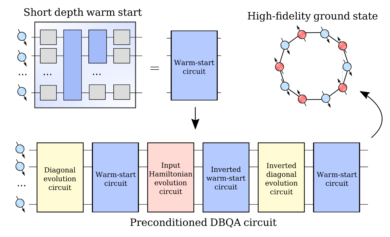
Quantum algorithm DB-QITE - iterate recursively:
- Define \(|{\psi_k}\rangle = U_k |0\rangle\)
- Use \(e^{is |\psi_k\rangle\langle\psi_k|} = U_ke^{is |0\rangle\langle0|}U_k^\dagger \)
- Recursively iterate \( U_{k+1} = e^{is H} U_k e^{is |0\rangle\langle 0|} U_k^\dagger e^{-is H} U_k\)
3 stages of creating quantum algorithms
1. Design choice:
How to go about it?
3. Circuit compilation:
What gates to do?
|\psi(\tau)\rangle = \frac{e^{-\tau H}|\psi\rangle}{\| e^{-\tau H}|\psi\rangle\|}
0. Problem choice:
What challenge to take up?
e^{itH}\\
e^{it|\psi\rangle\langle\psi|}
4 stages of creating quantum algorithms
2. Unitary synthesis:
How to do it?

(accepted at PRL)
3. Circuit compilation:
What gates to do?
Product formula approximation:
\(e^{\tau[|\psi\rangle\langle\psi|,H]} = e^{i\sqrt{\tau}H}e^{i\sqrt{\tau}|\psi\rangle\langle\psi|}e^{-i\sqrt{\tau}H}e^{-i\sqrt{\tau}|\psi\rangle\langle\psi|} + O(\tau^{3/2})\)
Quantum algorithm DB-QITE - iterate recursively:
- Define \(|{\psi_k}\rangle = U_k |0\rangle\)
- Use \(e^{is |\psi_k\rangle\langle\psi_k|} = U_ke^{is |0\rangle\langle0|}U_k^\dagger \)
- Recursively iterate \( U_{k+1} = e^{is H} U_k e^{is |0\rangle\langle 0|} U_k^\dagger e^{-is H} U_k\)
3 stages of creating quantum algorithms
1. Design choice:
How to go about it?
3. Circuit compilation:
What gates to do?
|\psi(\tau)\rangle = \frac{e^{-\tau H}|\psi\rangle}{\| e^{-\tau H}|\psi\rangle\|}
0. Problem choice:
What challenge to take up?
e^{itH}\\
e^{it|\psi\rangle\langle\psi|}
4 stages of creating quantum algorithms
2. Unitary synthesis:
How to do it?
(accepted at PRL)
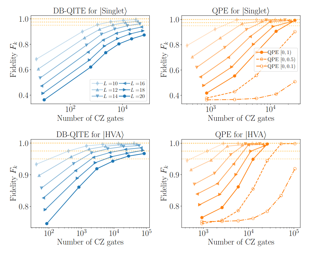
Numerical results for DB-QITE:
DB-QITE:
- Define \(|{\psi_k}\rangle = U_k |0\rangle\)
- Recursively iterate \( U_{k+1} = e^{is H} U_k e^{is |0\rangle\langle 0|} U_k^\dagger e^{-is H} U_k\)
Then:


Quantinuum
(accepted at PRL)
4 stages of creating quantum algorithms
1. Design choice:
How to go about it?
|\psi(\tau)\rangle = \frac{e^{-\tau H}|\psi\rangle}{\| e^{-\tau H}|\psi\rangle\|}
3. Circuit compilation:
What gates to do?
0. Problem choice:
What challenge to take up?
2. Unitary synthesis:
How to do it?
Double-bracket quantum algorithms:
Systematic framework for unitary synthesis
4 stages of creating quantum algorithms
Double-bracket quantum algorithms
Click these links at slides.com/marekgluza
| Diagonalization | https://arxiv.org/abs/2206.11772 | ||
|---|---|---|---|
| Imaginary-time evolution | https://arxiv.org/abs/2412.04554 | ||
| Quantum signal processing | https://arxiv.org/abs/2504.01077 | ||
| Grover's search | https://arxiv.org/abs/2507.15065 | Approximates ITE |
U^\dagger H U =
\begin{pmatrix}
\lambda_0&&\\
&\lambda_1&\\
&&\ddots
\end{pmatrix}
|\psi(\tau)\rangle = \frac{e^{-\tau H}|\psi\rangle}{\| e^{-\tau H}|\psi\rangle\|}
\frac{ \prod_{k=1}^K(H-z_k I)|\psi\rangle}{\| \prod_{k=1}^K(H-z_k I)|\psi\rangle\|}
\prod_{k=1}^Ke^{i\theta_k|\psi_k\rangle\langle\psi_k|} e^{s_k[|\psi_k\rangle\langle\psi_k|,H]}|\psi\rangle
H' = e^{-s[D,H]}H e^{s[D,H]}
e^{s[|\psi\rangle\langle\psi|,H]}|\psi\rangle +O(\tau^2)
(1-2|\psi\rangle\langle\psi|)\times e^{i t H_f}
e^{s[|\psi\rangle\langle\psi|,H]}|\psi\rangle
Solve the unitary synthesis problem in all these cases through Riemannian gradients!
Double-bracket quantum algorithms
- Coherently implement Riemannian gradient steps
-
Give rigorous unitary synthesis for
- imaginary-time evolution
- quantum signal processing
- diagonalization unitaries
- Grover's as an approximation to imaginary-time evolution
- Training quantum circuits from data doesn't work well, unlike in classical machine learning applications. However those variational learning methods are great for warm-starting double-bracket quantum algorithms!
Tell me when not fast enough? Get stuck? Something else?
Your input is needed to improve them!
N. Ng
Z. Holmes
R. Zander

R. Seidel
Y. Suzuki
B. Tiang
J. Son
S. Carrazza
Stay in touch on LinkedIn:
Text
Text
Text
Marek Gluza
The double-bracket quantum algorithms roadmap
I grew up around these mountains where Poland meets Czech Republic and Slovakia (in Europe)
June '22: Single-author double-bracket proposal

This talk is an overview of 4 years of my research on double-bracket quantum algorithms:
- Never worked on quantum algorithms before \(\rightarrow\) 9 papers, 1 experiment
- Never participated in a research program \(\rightarrow\) lead a collaboration of 25 co-authors
- It was the mathematical observations guiding us \(\rightarrow\) Riemannian geometry is key!
[1]
[9]
[8]
[5]
[2]
[3,4]
[6]
[7]
Click these links at slides.com/marekgluza

October '21: Arrived to Singapore
How to go about designing quantum algorithms?
- Now: Not many distinct quantum algorithms
https://quantumalgorithmzoo.org/ - Why?
- Classically: Reduction to decision problems
- Quantumly: Is \(\langle\psi|H|\psi\rangle\) lower than ...?
- Optimization: Only quadratic speed-up?
- "Grand unification of quantum algorithms" https://arxiv.org/abs/2105.02859 the block-encoding scheme for accessing \(H\)
- This talk: Another unification based on Riemannian optimization and using geodesics \(e^{isH}\) to access \(H\)
- Double-bracket quantum algorithms give intuition why unification possible: \(\langle\psi|H|\psi\rangle\) is optimization so interpret through Riemannian gradients
Click links at slides.com/marekgluza
E(\psi) = \langle \psi| H | \psi\rangle
="\overline{v}^\top H v"
Marek Gluza
The double-bracket quantum algorithms roadmap
...the outline of the talk
Today, I will tell you about double-bracket quantum algorithms
Part 1:
- What are quantum algorithms?
- What is quantum computing?
Part 3:
- What can they be used for?
- What are good tasks for quantum computers?
Part 2:
- Riemannian geometry of the unitary group
Part 4: Just basic properties of the unitary group facilitate quantum algorithm design
New quantum algorithms based on Riemannian optimization
Marek Gluza
NTU Singapore
Scan QR code or go to slides.com/marekgluza
Watch on youtube: https://www.youtube.com/watch?v=PLVkuqPemVs
What is a quantum computer?
It is a quantum system e.g. ionized atom, loop of a superconductor
|
|
|
|---|---|
|
|
|
|
|
|
|
|
|
|
|
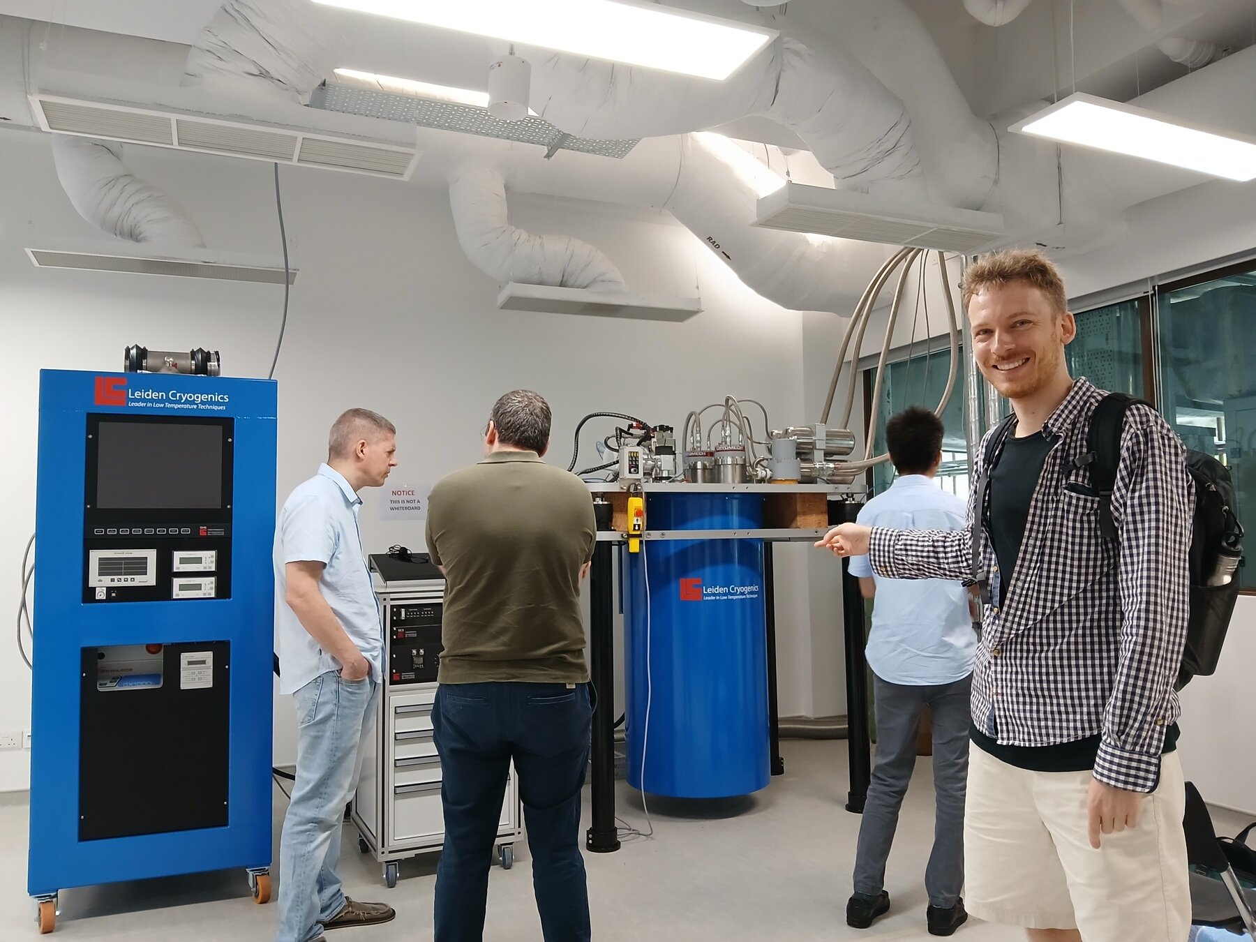
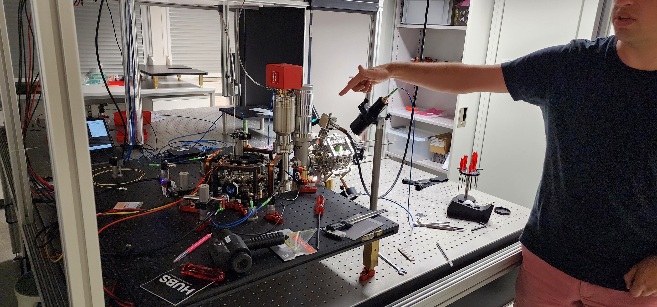
J. Leonard (TU Vienna) pointing where neutral atoms will be trapped
R. Dumke and S. Carrazza discussiong the CQT lab
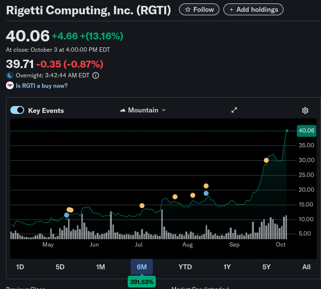
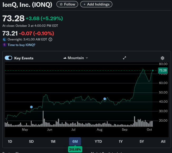
Some investors speculate their money on it - RGTI, IONQ...
We can make it!

What is a quantum computer?
It is a quantum system e.g. ionized atom, loop of a superconductor
It is modeled by a finite dimensional vector space \(\mathcal V = \mathbb C^d\)
It is modular: We can add more of its components and make \(d\) grow
It is programmable: There are ways (quantum gates) to change its states in a reproducible and reversible manner
It is universal: Composing sufficiently many of the programmable operations allows to approximate any \(|v\rangle \in \mathcal V\)
We take more qubits
Apply patterned EM radiation
Reproducible: Use FPGA
Reversible: Physics challenge; keep cold
|
|
|
|---|---|
|
|
|
|
|
|
|
|
|
|
|
We can make it!
We take \(n\) qubits then \(\mathcal V = (\mathbb C^2)^{\otimes n}\) and \(d=2^n\)
Physics papers from the 90's
For good or for worse quantum computing is influenced by physics...
How to go about designing quantum algorithms?
- Now: Not many distinct quantum algorithms
https://quantumalgorithmzoo.org/ - Why?
- 00's Shor: Why have not more algorithms been found?
https://cs.brynmawr.edu/Courses/cs380/fall2012/Shor2003.pdf
Either because the easy ones are efficient classically or we have no good language
- Classically: Reduction to decision problems
- Quantumly: Is \(\langle\psi|H|\psi\rangle\) lower than ...?
- Optimization: Only quadratic speed-up?
Click links at slides.com/marekgluza
- 90's Shor: quantum computers can break cryptography
E(\psi) = \langle \psi| H | \psi\rangle
="\overline{v}^\top H v"
Why materials science? Imagine improving photovoltaics by 1%.
What needs to be done? Perform \(\bra\psi H\ket\psi\) optimization.
How? Quantum circuit synthesis.
This is worth being hyped!
Materials science?
What is a quantum algorithm?
0
0
0
0
C
What is a quantum computer?
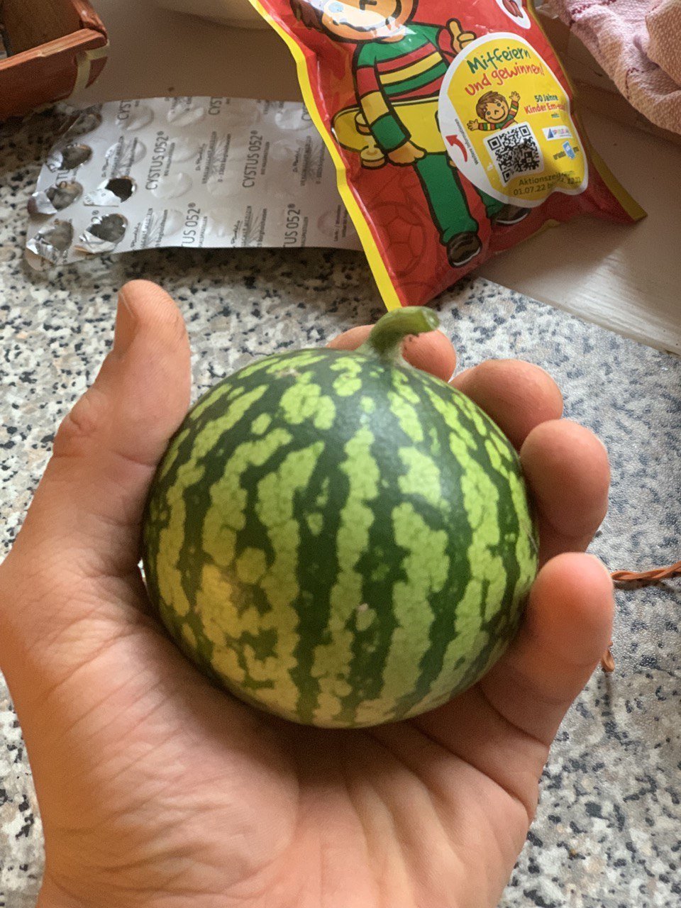
It's an experimental setup A which includes a quantum system B and that setup A allows to manipulate the quantum state of B.
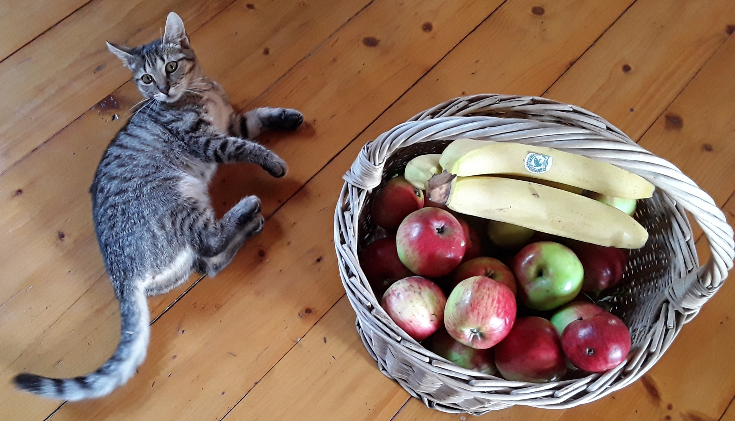
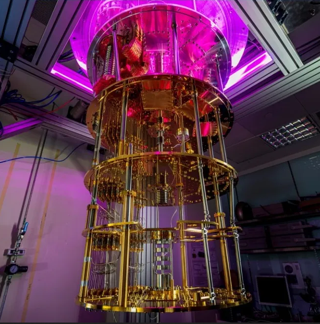
(This monumental structure is the insides of the dilution refrigerator shielding qubits from noise)
A - basket
B - fruits
Cat - noise
A - quantum computer
B - qubits
C - noise
Quantum Dynamic Programming in Qibo
How to use quantum computers programmed by quantum information?
Can quantum states program a quantum computer?
Can quantum information be the source code?
What would it be good for?

Introduction
What is a dynamic quantum algorithm?
Dynamic Quantum Algorithm
- Consider a data qubit and an instruction qubit
- Make an infinitesimal rotation by Heisenberg hamiltonian on these 2 qubits
- Discard the instruction qubits and prepare a fresh copy of that instruction state
- Repeat the Heisenberg evolution and fresh preparation
- If the infinitesimal rotation duration is dt then after M steps we will have
- The circuit will be exactly the same even if we use different qubit states
\sigma \to e^{idtM\rho}\sigma e^{-idtM\rho} + O(M^{-1})
XX + YY + ZZ
\sigma
\rho
Density Matrix Exponentiation
- Consider a data qubit and an instruction qubit
- Make an infinitesimal rotation by applying partial SWAP (\(\delta\)SWAP) gate, realized by Heisenberg interaction
- Discard the instruction qubits and prepare a fresh copy of that instruction state.
- Since density matrix \(\rho\) is Hermitian, we can use it as an operator: \(\sigma \to e^{-i\rho\delta}\sigma e^{i\rho\delta}\)
- Repeat the partial SWAP and fresh preparation
- If the infinitesimal rotation duration is dt then after M steps we will have
\sigma \to e^{idtM\rho}\sigma e^{-idtM\rho} + O(M^{-1})
XX + YY + ZZ
\sigma
\rho
Density Matrix Exponentiation
- Since density matrix \(\rho\) is Hermitian, we can use it as an operator
- DME implements am infinitesimal unitary rotation about an axis defined by instruction qubit 𝜌 on data qubit 𝜎:\[e^{-i\rho\delta}\sigma e^{i\rho\delta}\]
- After Trotterization, DME implements: \(U = e^{-i\rho\theta}\)
- Again, this is dynamic because \(\rho\) is only determined at runtime
Dynamic Quantum Algorithm
- Quantum algorithms that are dynamic: their operation is revealed on runtime.
- Dynamic quantum algorithm: Algorithm that take an unknown density matrix and design a circuit that will meaningfully use this quantum information as an instruction
- Kimmel et al. (arxiv 1608.00281) shows that this model is basis of a universal model for quantum computation
- Example usage: there is a universal circuit that compute the Schmidt spectrum
Static vs Dynamic

Kjaergaard et al., 2001.08838
- Usual quantum computing is static: To change operation, we have to change the circuit
- Our approach (dynamic quantum computing) is dynamic: To change operation, only need to change instruction qubit
Existing literature
Kjaergaard et al., 2001.08838
Motivation for
Quantum Dynamic Programming
What is Quantum Dynamic Programming (QDP) good for?
What is a quantum recursion
- Definition:
- More complicated, dynamic case:
As we are taking more steps, the recursive state is instructing the propagation - Problem:
- What is a meaningful \(U(\psi)\)?
- To calculate \(\ket {\psi''}\) will we need to recalculate \(\ket {\psi'}\) and calculate \(U(\psi')\)?
- For higher order terms, do we need to recalculate all lower terms?
\ket{\psi'} = U(\psi) \ket \psi\\
U(\psi) \neq U(\psi')\\
\text{if } \psi \neq \psi'
\ket{\psi''} = U(\psi') \ket{\psi'}\\
Quantum recursion examples
- Solution: QDP shows how to do it in a quantum coherent way.
- Examples of quantum recursions:
- Grover rotation: \[G=id - 2\ket\psi\bra\psi\]
G(ψ1)=U0†G(ψ0)U0=id−2∣ψ1⟩⟨ψ1∣G^{(\psi_1)} = U_0^\dagger G^{(\psi_0)}U_0=\mathbb{id} - 2\ket{\psi_1}\bra{\psi_1} - Grover search: Add static unitaries Q and R that don’t depend on the state:
\(U^{(\psi)} = QG^{(\psi)}R\) with \(Q,R\in U(D)\) - Density Matrix Exponentiation: Explain dynamic Grover rotation implementation: \[G = e^{i\psi s}\]
- Grover rotation: \[G=id - 2\ket\psi\bra\psi\]
Quantum recursion examples
- Reduced group commutator: Approximate commutator evolution and similar structures that evolve with density matrix.
\[e^{isD}e^{it\rho}e^{-isD}\] - We can use this to diagonalize
eisDeitρe−isDe^{isD}e^{it\rho}e^{-isD}

Marek DBI paper, arxiv 2206.11772
QDP paper, arxiv 2403.09187
Unfolding quantum recursions
Consider Grover reflector: \(G=id - 2\ket\psi\bra\psi\)
\(Q,R \in U(D)\), initial state \(\ket{\psi_0}\), \(\ket{\psi_{k+1}} = QG^{(\psi_k)}R\ket{\psi_k}\)
To get \(\ket{\psi_1}\) is simple:
\begin{align*}
G^{(\psi_1)} &= U_0^\dagger G^{(\psi_0)}U_0\\
&=\mathbb{1} - 2\ket{\psi_1}\bra{\psi_1}\\
&=\mathbb{1} - 2U_0 \ket{\psi_0}\bra{\psi_0}U_0^\dagger\\
&=U_0(\mathbb{1}-2\ket{\psi_0}\bra{\psi_0})U_0^\dagger\\
\ket{\psi_2} &= QG^{(\psi_1)}R\ket{\psi_1}\\
&=\boxed{QU_0(\mathbb{1}-2\ket{\psi_0}\bra{\psi_0})U_0^\dagger R QG^{(\psi_0)}R\ket{\psi_0}}
\end{align*}
\begin{align*}
U(\psi_0) &= QG^{(\psi_0)}R\\
\ket{\psi_1} &= QG^{(\psi_0)}R\ket{\psi_0}
\end{align*}
However, it's more complicated to get \(\ket{\psi_2}\). Ordinary idea:
Motivation for QDP
- Unfolding the recursion make the depth grow exponentially
- Using placeholder memory is not straightforward with quantum computing
- Notice that the unitary \(U(\psi)\) depends on \(\ket\psi\). Can we use the state to steer the evolution?
- Quantum Dynamic Programming (QDP), a framework that uses copies of the recursive state to implement the recursion step unitary
- This is dynamic because the instruction state is revealed only on runtime
- QDP yields exponential reduction in circuit depth than when unfolding
Quantum Dynamic Programming
J. Son et al, arxiv 2403.09187

Quantum Dynamic Programming
- Simple case: Recursion step unitary that make a single memory call
\[ U^{(\mathcal{N},\rho)} = V_2e^{i\mathcal{N}(\rho)}V_1\] where \(\mathcal{N}\) is the operator of the memory call - General case: Repeat this many times for the same instruction state
- Memory call: the step is asking for memory (instruction state \(\rho\))
- Problem: We can't implement this naturally in qunatum mechanics
Quantum Dynamic Programming
- Solution: QDP approximate this memory call unitary:
- QDP does this by using memory usage query:
where \(N\) is the unitary of the memory usage query - Memory usage query: consume (trace out) an instruction state
- Repeat this procedure M times, we obtain
\mathcal{E}_s^{(N,\rho)}(\sigma) = Tr_\rho [e^{-iNs} (\rho\otimes\sigma) e^{iNs}]
E^{(\mathcal{N},\rho)}(\sigma) = e^{i\mathcal{N}(\rho)} \sigma e^{-i\mathcal{N}(\rho)}
\mathcal{E}^{(\mathcal{N},\rho,M)}_{QDP} \coloneqq (\mathcal{E}^{(\mathcal{N},\rho)}_{1/M})^M = E^{(\mathcal{N},\rho)} + O(1/M)
Density Matrix Exponentiation (DME) in Qibo
Memory usage query in DME
- Goal: DME approximate the rotation (the memory call):
\[U = e^{-i\rho\theta}\] - DME replace the infinitesimal angle memory call unitary (where \(\delta = \theta/N\)): \[\sigma\to e^{-i\rho\delta}\sigma e^{i\rho\delta}\] by the memory usage query \[\sigma\to\text{Tr}_\rho[e^{-i\text{SWAP}\delta}(\sigma\otimes\rho) e^{i\text{SWAP}\delta}]\]
-
DME then does \(N\) memory usage queries (Trotterization):
DME(\rho,N,\theta) = e^{-i\rho\theta} + O\left(\frac{\theta^2}{N}\right)

DME flowchart

\text{Tr}_\rho[e^{-i\text{SWAP}\delta}(\sigma\otimes\rho) e^{i\text{SWAP}\delta}] \\
= e^{-i\rho\delta}\sigma e^{i\rho\delta}+O(\delta^2)
Problem of Entanglement
- To use quantum info from \(\rho\), we need it to interact and correlate with \(\sigma\)
- How do we avoid entanglement between \(\rho\) and \(\sigma\)?
- Example: the Bell state circuit create entanglement

How DME avoid entanglement
- DME uses a series of partial SWAP gate, realized by Heisenberg interaction: \(H_{\text{Heisenberg}} = e^{it{(XX + YY + ZZ)}}\)
- DME relies on the relation:
- Where, after the partial SWAP, by tracing out the instruction qubit, we get in first order the desired rotation
- The data qubit is in a pure state since the rotation is infinitesimal

DME in Qibo
DME tutorial notebook

QDP code structure

Github PR #1302
QDP code structure
- There are 2 important parts of a QDP circuit:
- Memory call circuit: How many instruction qubit to use, how to get N copies of the instruction qubit
- Memory usage query (circuit): Define the operator used to generate the unitary rotation (in the case of DME the 𝛿SWAP)

Conclusion
Conclusion
- How to use quantum computers programmed by quantum information?
- Can quantum states program a quantum computer? Can quantum information be the source code?
- What would it be good for?
- What is a dynamic quantum algorithm? What is QDP?
- What is DME? How does DME work?
- The QDP code structure?
Quantum algorithms for optimisation derived from the non-Euclidean geometry of quantum computing operations
By Marek Gluza
Quantum algorithms for optimisation derived from the non-Euclidean geometry of quantum computing operations
In this talk we will explore how to use non-Euclidean geometry as guidance to propose how to perform optimization through quantum computing. Here, the allowed operations are rotations of vectors which preserve their lengths, i.e. unitary matrices, and we will use their geometric properties to find protocols which implement the paradigmatic imaginary-time evolution known from quantum field theory. We will interpret the resulting quantum algorithm geometrically as a progression of states evolving in the direction of the steepest decrease of the energy cost function. This result is part of a larger program on double-bracket quantum algorithms and I will briefly list our other findings so far. I will then sketch the plans for our collaboration with the members of the Siam Quantum Square, warmly inviting you to join us.


