How rotations on spheres can help you think about quantum computation
Marek Gluza
Nanyang Technological University
Singapore
What is a quantum computer?
It is a quantum system e.g. ionized atom, loop of a superconductor
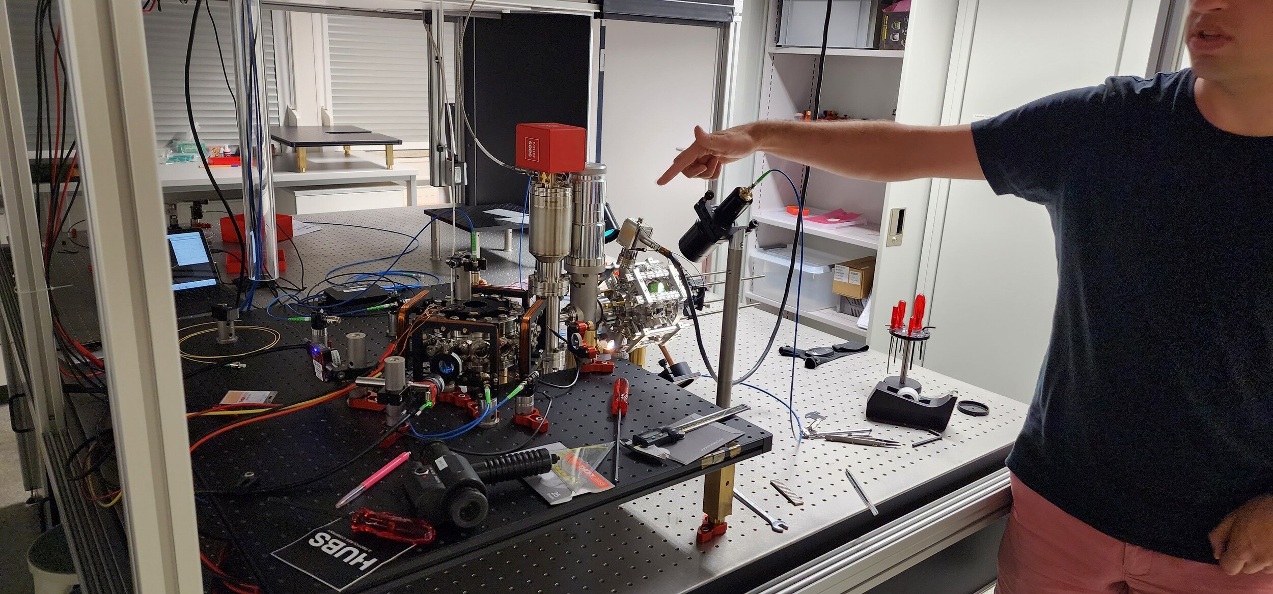
J. Leonard (TU Vienna) pointing where neutral atoms will be trapped
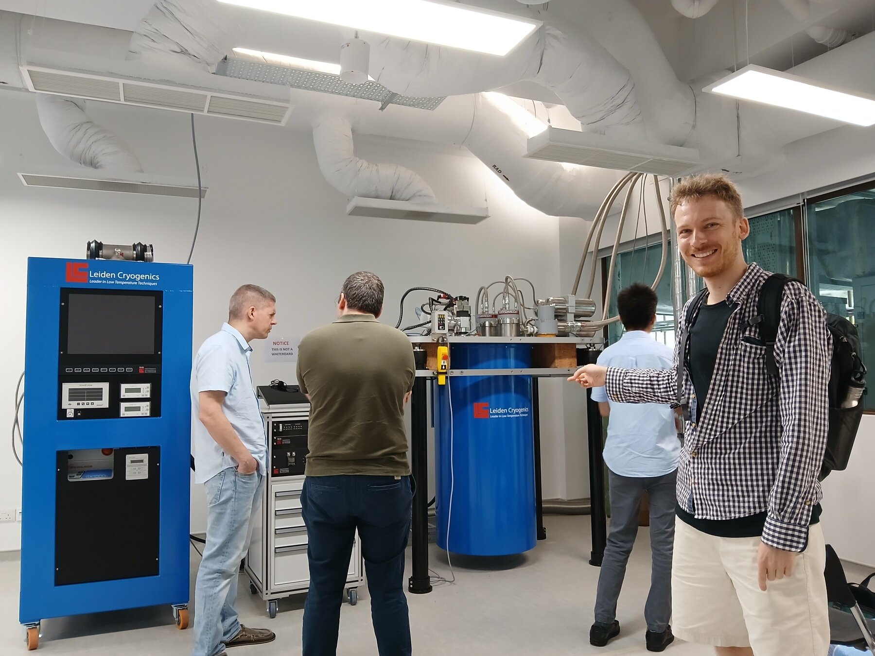
R. Dumke and S. Carrazza discussiong the CQT lab
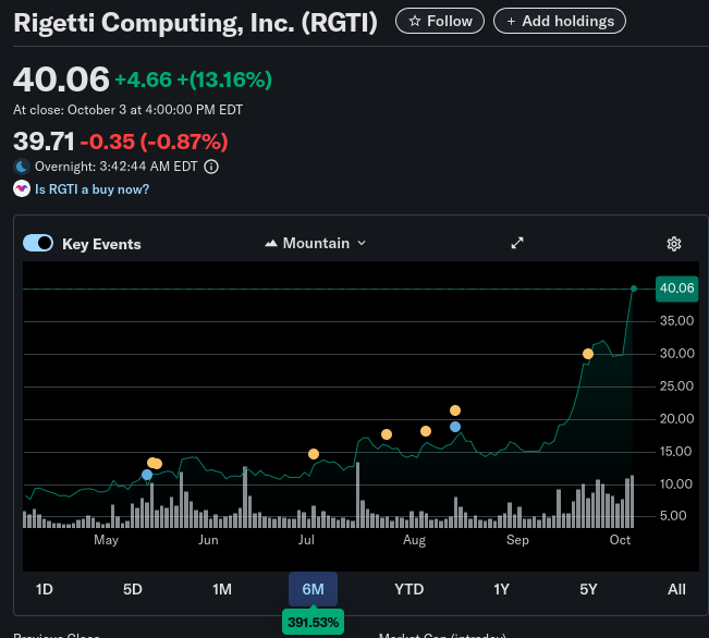
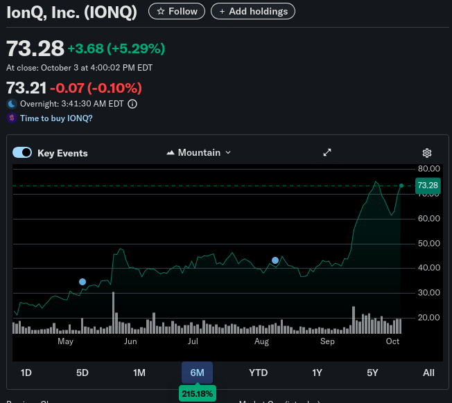
Some investors speculate their money on it - RGTI, IONQ...
We can make it!

What is a quantum computer?
It is a quantum system,e.g.
ionized atom, loop of a superconductor
It is a quantum system modelled by vectors
It is modular: We can add more of its components and make \(d\) grow
It is programmable: There are ways (quantum gates) to change its states in a reproducible and reversible manner
It is universal: Composing sufficiently many quantum gates allows to reach any vector you want \(\vec v = |\psi\rangle \)
We take more qubits
Apply patterned EM radiation
Reproducible: Use FPGA
Reversible: Physics challenge; keep cold
Physics papers from the 90's
We can make it!
\(\vec{v} = \begin{pmatrix} x \\ y \end{pmatrix}\)
\(\ket{\psi} = \begin{pmatrix} x \\ y \\z \\k\end{pmatrix} = \begin{pmatrix} 0.5 \\[4pt] 0.5 \\[4pt] 0.5 \\[4pt] 0.5 \end{pmatrix}\)
What is a quantum computer?
It is a quantum system,e.g.
ionized atom, loop of a superconductor
It is a quantum system modelled by vectors
It is modular: We can add more of its components and make \(d\) grow
It is programmable: There are ways (quantum gates) to change its states in a reproducible and reversible manner
It is universal: Composing sufficiently many quantum gates allows to reach any vector you want \(\vec v = |\psi\rangle \)
We take more qubits
Apply patterned EM radiation
Reproducible: Use FPGA
Reversible: Physics challenge; keep cold
Physics papers from the 90's
We can make it!
\(\vec{v} = \begin{pmatrix} x \\ y \end{pmatrix}\)
\(\ket{\psi} = \begin{pmatrix} x \\ y \\z \\k\end{pmatrix} = \begin{pmatrix} 0.5 \\[4pt] 0.5 \\[4pt] 0.5 \\[4pt] 0.5 \end{pmatrix}\)
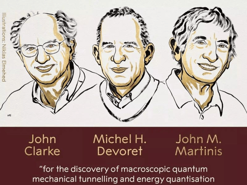
For good or for worse quantum computing is influenced by physics...
0
0
0
0
C
What is a quantum computer?
It's an experimental setup A which includes a quantum system B and that setup A allows to manipulate the quantum state of B. This is modelled by rotating vectors.
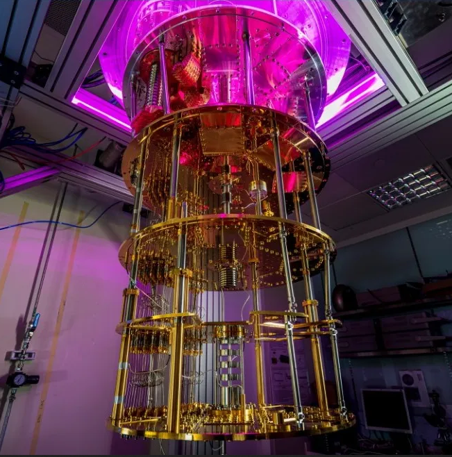
(This monumental structure is the insides of the dilution refrigerator shielding qubits from noise)
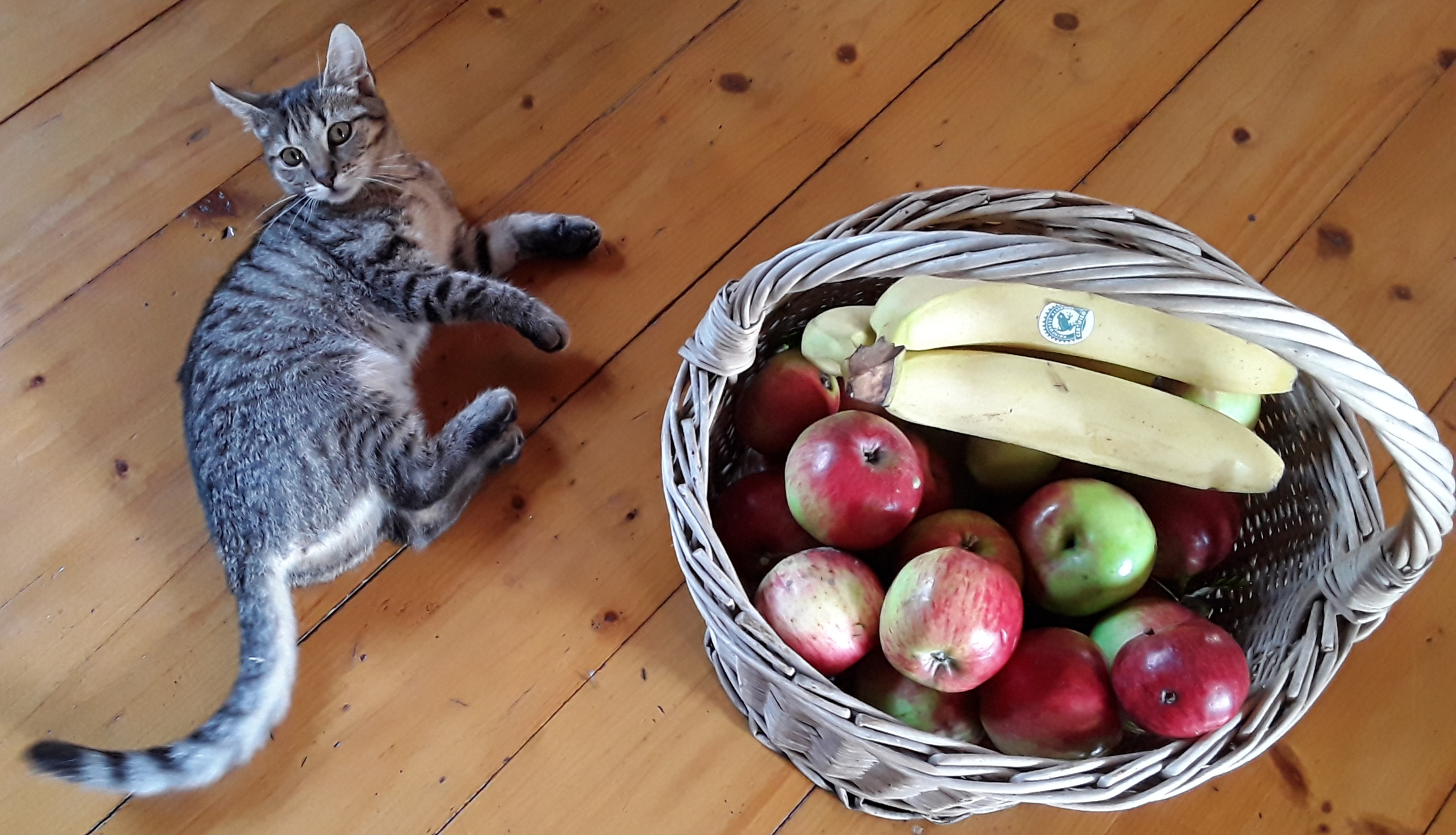
A - basket
B - fruits
Cat - noise
A - quantum computer
B - qubits
C - noise
This visualizes the operations on a quantum computer
(Riemannian geometry)
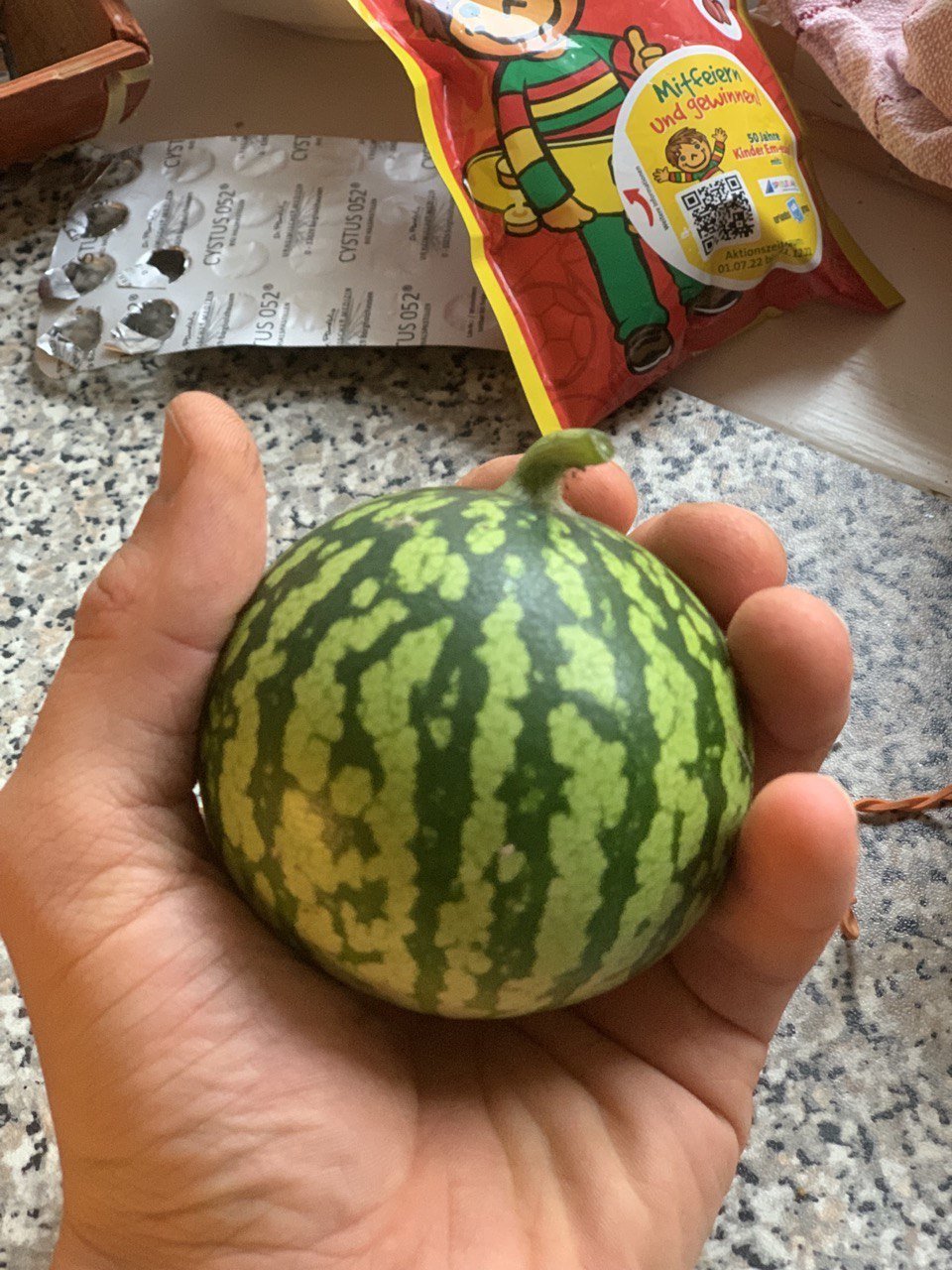
- Riemannian geometry is a generalization of the geometry of the sphere
- For 1 qubit the sphere is a great model of quantum operations
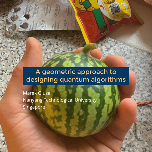
- In higher dimensions many parallels remain e.g. set of quantum operations is compact (the watermelon fits into the hand) but many get lost e.g. non-convex submanifolds (green colors on the watermelon)
- If watermelon is placed on the table then the table is tangent to it
How to use geometry to design quantum algorithms?
4 stages of creating quantum algorithms
Guidelines for using quantum computing
Stage 1: Think. What is the goal?
Important problems that are difficult yet doable.
Encode what we know in \(\vec{v}_{input}\).
Decode information from \(\vec{v}_{output}\).
Find effective heuristics to reduce the runtime of rotations \(R_k\)
Find rotations such that
\(\vec{v}_{output} \approx R_1 R_2 \ldots R_n \vec{v}_{input}\)
Stage 2: Design. How to encode task in quantum mechanics?
|\psi(\tau)\rangle = \frac{e^{-\tau H}|\psi\rangle}{\| e^{-\tau H}|\psi\rangle\|}

Stage 4: Run it.
What instructions to send?
Stage 3: Algorithm. How to find \(\vec{v}_{output}\)?
Guidelines for extracting utility from quantum computing
Stage 1: Think. What is the goal?
Stage 4: Run it.
What instructions to send?
Stage 2: Design. How to encode task in quantum mechanics?
Stage 3: Algorithm. How to find \(\vec{v}_{output}\)?
Quantum computing cannot be useful if
- The problem can be solved quickly on classical computers
- Solving the problem isn't important
- Solving the problem is too hard for the quantum computer
Classical computation
Key question in current quantum computation:
Find an important problem which is difficult yet doable
Millenials doing quantum computing
What challenge to take up?
4 stages of creating quantum algorithms
Guidelines for using quantum computing
Stage 1: Think. What is the goal?
Stage 2: Design. How to encode task in quantum mechanics?
|\psi(\tau)\rangle = \frac{e^{-\tau H}|\psi\rangle}{\| e^{-\tau H}|\psi\rangle\|}
Stage 4: Run it.
What instructions to send?
Stage 3: Algorithm. How to find \(\vec{v}_{output}\)?
Mathematically, states of the quantum computer are like arrows pointing from the center of the sphere to its surface.
Observation leading to double-bracket quantum algorithms: Earth is not flat. I.e., when we walk along of the equator, we think we are going straight but eventually we will wrap around it.
Fixing a direction and rotating the arrow, corresponds to a type of of quantum computing operation.
Stage 3: Algorithm. How to find \(\vec{v}_{output}\)?
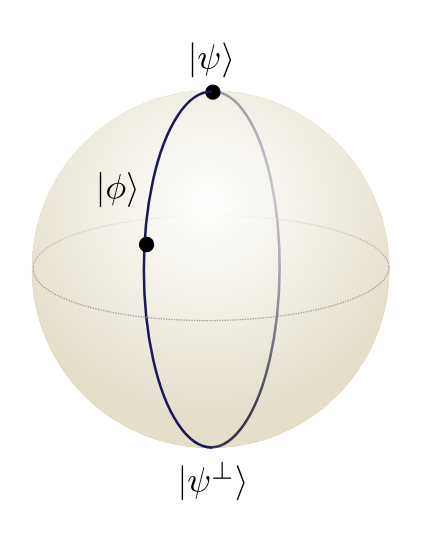
Riemannian geometry underlies quantum algorithms
On a flat surface DOWN-LEFT-UP-RIGHT will return to point of origin.
Stage 3: Algorithm. How to find \(\vec{v}_{output}\)?
Riemannian geometry underlying quantum algorithms
On a flat surface DOWN-LEFT-UP-RIGHT will return to point of origin.
On a curved surface SOUTH-WEST-NORTH-EAST will spiral way.
South
West
East
North
Stage 3: Algorithm. How to find \(\vec{v}_{output}\)?
Riemannian geometry underlying quantum algorithms
South
West
East
North
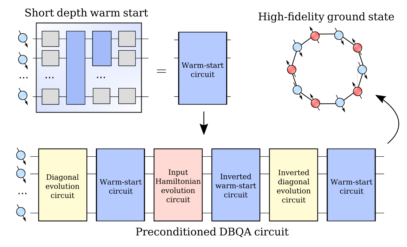
My work on double-bracket quantum algorithms shows how to use this spiraling effect to implement non-Euclidean gradient descent in quantum computing.
Regular machine learning fails for quantum computing but our generalization works. The 'failed' machine learning is still key for us - as a warm-start!

(Physical Review Letters '26)
Stage 3: Algorithm. How to find \(\vec{v}_{output}\)?
Riemannian geometry underlying quantum algorithms
Product formula approximation:
\(e^{\tau[|\psi\rangle\langle\psi|,H]} = e^{i\sqrt{\tau}H}e^{i\sqrt{\tau}|\psi\rangle\langle\psi|}e^{-i\sqrt{\tau}H}e^{-i\sqrt{\tau}|\psi\rangle\langle\psi|} + O(\tau^{3/2})\)
Quantum algorithm DB-QITE - iterate recursively:
- Define \(|{\psi_k}\rangle = U_k |0\rangle\)
- Use \(e^{is |\psi_k\rangle\langle\psi_k|} = U_ke^{is |0\rangle\langle0|}U_k^\dagger \)
- Recursively iterate \( U_{k+1} = e^{is H} U_k e^{is |0\rangle\langle 0|} U_k^\dagger e^{-is H} U_k\)
1. Design choice:
How to go about it?
4. Circuit compilation:
What gates to do?
|\psi(\tau)\rangle = \frac{e^{-\tau H}|\psi\rangle}{\| e^{-\tau H}|\psi\rangle\|}
0. Problem choice:
What challenge to take up?
e^{itH}\\
e^{it|\psi\rangle\langle\psi|}
NTU's DB-QITE quantum algorithm
2. Unitary synthesis:
How to do it?
(accepted at PRL)
Numerical results for DB-QITE:
DB-QITE:
- Define \(|{\psi_k}\rangle = U_k |0\rangle\)
- Recursively iterate \( U_{k+1} = e^{is H} U_k e^{is |0\rangle\langle 0|} U_k^\dagger e^{-is H} U_k\)
Then:


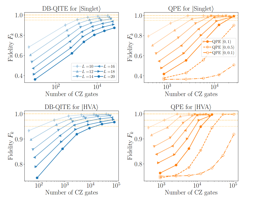
Quantinuum
(accepted at PRL)
4 stages of creating quantum algorithms
Guidelines for using quantum computing
Stage 1: Think. What is the goal?
Stage 2: Design. How to encode task in quantum mechanics?
|\psi(\tau)\rangle = \frac{e^{-\tau H}|\psi\rangle}{\| e^{-\tau H}|\psi\rangle\|}
Stage 4: Run it.
What instructions to send?
Stage 3: Algorithm. How to find \(\vec{v}_{output}\)?
Marek Gluza
The double-bracket quantum algorithms roadmap
I grew up around these mountains where Poland meets Czech Republic and Slovakia (in Europe)
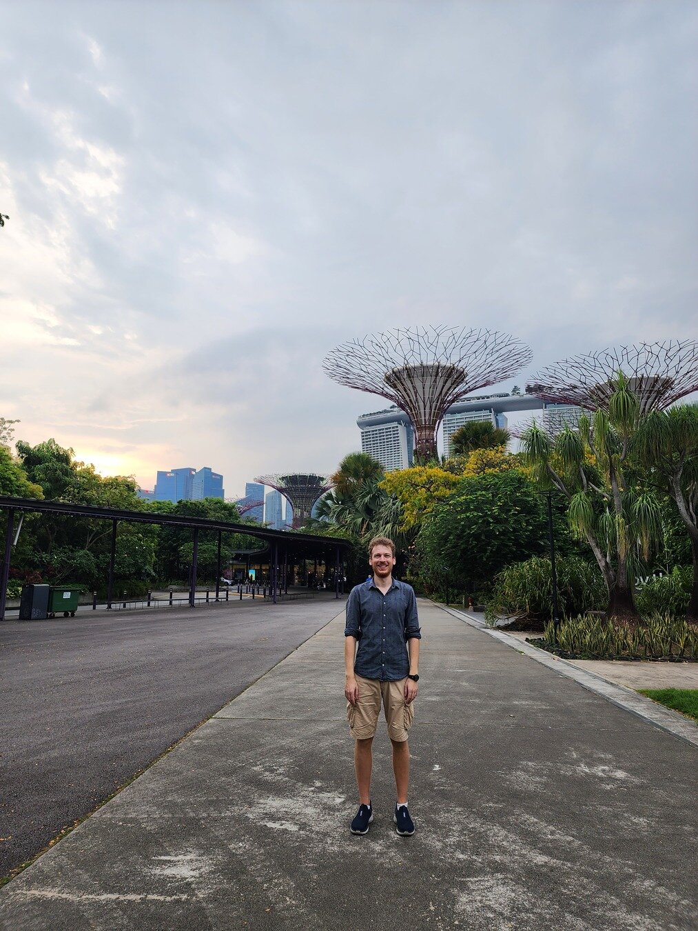
June '22: Single-author double-bracket proposal

This talk is an overview of 4 years of my research on double-bracket quantum algorithms:
- Never worked on quantum algorithms before \(\rightarrow\) 9 papers, 1 experiment
- Never participated in a research program \(\rightarrow\) lead a collaboration of 25 co-authors
- It was the mathematical observations guiding us \(\rightarrow\) Riemannian geometry is key!
[1]
[9]
[8]
[5]
[2]
[3,4]
[6]
[7]
Click these links at slides.com/marekgluza

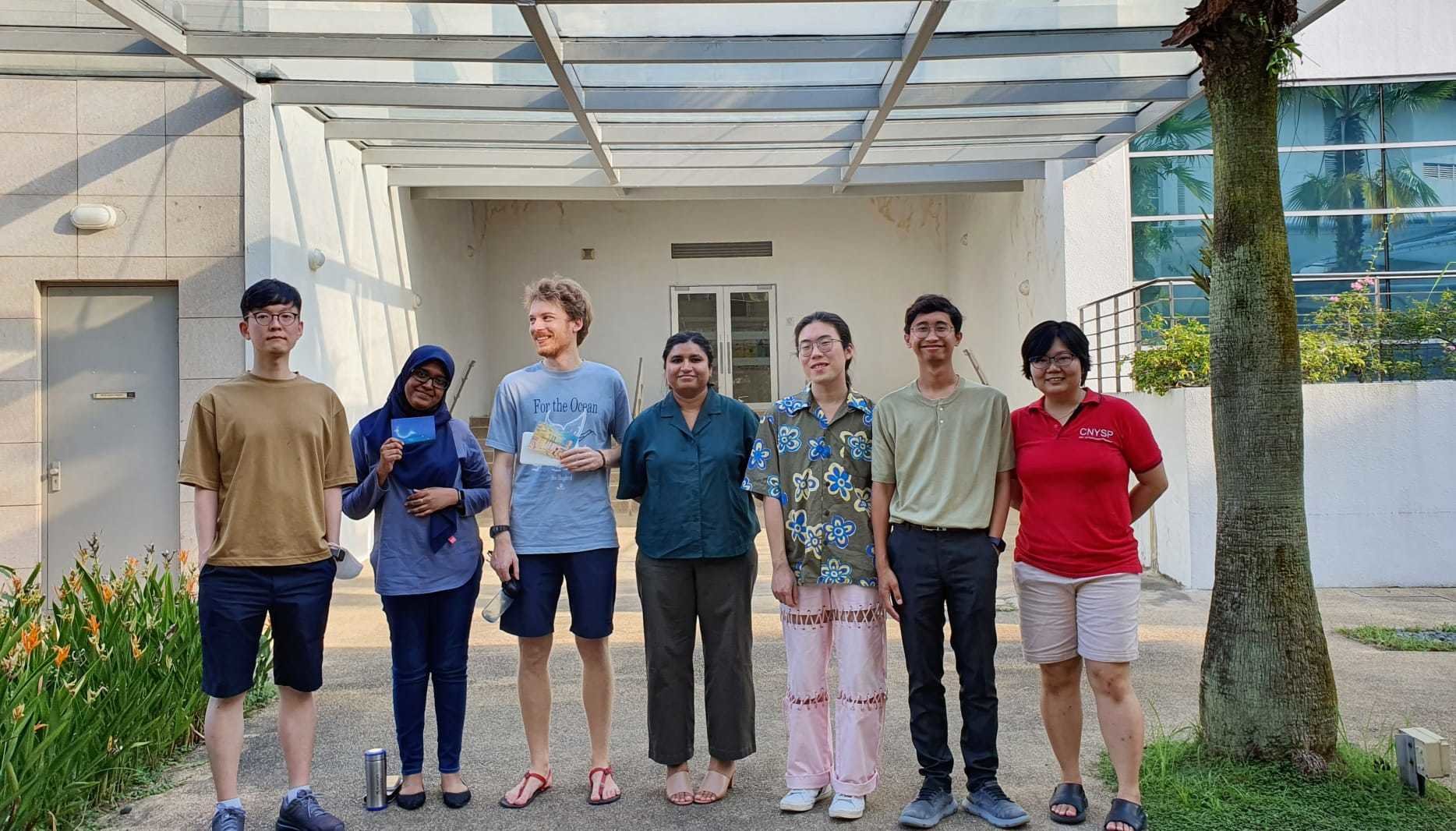

October '21: Arrived to Singapore
Marek Gluza
The double-bracket quantum algorithms roadmap
I grew up around these mountains where Poland meets Czech Republic and Slovakia (in Europe)
June '22: Single-author double-bracket proposal
This talk is an overview of 4 years of my research on double-bracket quantum algorithms:
- Never worked on quantum algorithms before \(\rightarrow\) 9 papers, 1 experiment
- Never participated in a research program \(\rightarrow\) lead a collaboration of 25 co-authors
- It was the mathematical observations guiding us \(\rightarrow\) Riemannian geometry is key!
[1]
[9]
[8]
[5]
[2]
[3,4]
[6]
[7]
Click these links at slides.com/marekgluza
October '21: Arrived to Singapore


Text
Stay in touch on LinkedIn:
Text
Text
4 stages of creating quantum algorithms
2. Design choice:
How to go about it?
|\psi(\tau)\rangle = \frac{e^{-\tau H}|\psi\rangle}{\| e^{-\tau H}|\psi\rangle\|}
4. Circuit compilation:
What gates to do?
1. Problem choice:
What challenge to take up?
3. Unitary synthesis:
How to do it?
4 stages of creating quantum algorithms
Quantum computing cannot be useful if
- The problem can be solved quickly on classical computers
- Solving the problem isn't important
- Solving the problem is too hard for the quantum computer
What challenge to take up?
Materials science?
Why materials science? Imagine improving photovoltaics by 1%.
What needs to be done? Perform \(\bra\psi H\ket\psi\) optimization.
How? Quantum circuit synthesis.
E(\psi) = \langle \psi| H | \psi\rangle
Key question in current quantum computation:
Find an important problem which is difficult yet doable
4 stages of creating quantum algorithms
2. Design choice:
How to go about it?
|\psi(\tau)\rangle = \frac{e^{-\tau H}|\psi\rangle}{\| e^{-\tau H}|\psi\rangle\|}
1. Problem choice:
What challenge to take up?
Double-bracket quantum algorithms:
Systematic framework for unitary synthesis
4 stages of creating quantum algorithms
E(\psi) = \langle \psi| H | \psi\rangle
4. Circuit compilation:
What gates to do?
3. Unitary synthesis:
How to do it?
4 stages of creating quantum algorithms
1. Design choice:
How to go about it?
|\psi(\tau)\rangle = \frac{e^{-\tau H}|\psi\rangle}{\| e^{-\tau H}|\psi\rangle\|}
3. Circuit compilation:
What gates to do?
|\psi(\tau)\rangle = \frac{e^{-\tau H}|\psi\rangle}{\| e^{-\tau H}|\psi\rangle\|}
0. Problem choice:
What challenge to take up?
2. Unitary synthesis:
How to do it?
4 stages of creating quantum algorithms
Imaginary-time evolution
\ket\psi\mapsto |\psi(\tau)\rangle
H = \sum_{k=1}^{D} \lambda_k \ket{\lambda_k}\bra{\lambda_k}
e^{-\tau H}|\psi\rangle = \langle\lambda_0|\psi\rangle \ket{\lambda_0} +\sum_{k=1}^{D} e^{-\tau\lambda_k} \langle\lambda_k|\psi\rangle \ket{\lambda_k}
|\psi\rangle = \langle\lambda_0|\psi\rangle \ket{\lambda_0} +\sum_{k=1}^{D} \langle\lambda_k|\psi\rangle \ket{\lambda_k}
\lim_{\tau\rightarrow \infty}\ket{\psi(\tau)} = \ket{\lambda_0}
Riemannian geometry is essential for quantum computation
- The unitary group \(U(d)\) is a Riemannian manifold
- It is an embedded manifold \(U(d) = \{M\in \mathbb C^{d\times d}:~M^{-1}=M^\dagger\}\)
- The tangent space is \(\{W\in \mathbb C^{d\times d}:~W^{\dagger}= -W\} \simeq\{iH \mathrm{~where~} H=H^\dagger\in \mathbb C^{d\times d}\} \)
- The geodesics are matrix exponentials \( \{e^{sW}\}_{s\in\mathbb R} \subset U(d)\) or \( \{e^{isH}\}_{s\in\mathbb R} \subset U(d)\)
- Computing a "gradient" must output an element of the tangent space
\mathbb C^{d\times d}
U(d)
g
W
iH
g^\dagger = -g
e^{s g}
g
g^\dagger = -g
\(\partial_{i,j}\) points to the interior, not tangential
Keep this in mind for later: Unlike in flat space, these 4 steps spiral away from the point of origin
Riemannian geometry is essential for quantum computation
- The unitary group \(U(d)\) is a Riemannian manifold
- The tangent space is \(\{H\in \mathbb C^{d\times d}:~H^{\dagger}= H\} \)
- The geodesics are matrix exponentials \( \{e^{isH}\}_{s\in\mathbb R} \subset U(d)\)
- \(U(d)\) is a curved manifold
e^{is A}e^{is B}e^{-is A}e^{-is B} \neq 1
e^{is A}
e^{isB}
e^{-isB}
e^{-is A}
Operating a quantum computer is all about the group of unitary matrices
\forall A=A^\dagger, B=B^\dagger: ~~M = e^{ [A,B]}\in U(d)
Think of rotations on a sphere
The Lie bracket of two 'velocities' is again a velocity:
Check: \([A,B]^\dagger = (AB- BA)^\dagger = B^\dagger A^\dagger -A^\dagger B^\dagger = -[A,B]\)
M^\dagger = (e^{ [A,B]})^\dagger = e^{ [A,B]^\dagger}=e^{ -[A,B]}=M^{-1}
U(d)
e^{ [A,B]}
\([A,B]^\dagger = -[A,B]\)
Check: \([A,B]^\dagger = -[A,B]\)
U(d) = \{ M\in \mathbb C^{d\times d}: M^{-1} = M^\dagger\}
Operating a quantum computer is all about the group of unitary matrices
\forall A=A^\dagger, B=B^\dagger: ~~M = e^{ [A,B]}\in U(d)
Think of rotations on a sphere
Fact 3: The Lie bracket of two 'velocities' is again a velocity
U(d) = \{ M\in \mathbb C^{d\times d}: M^{-1} = M^\dagger\}
e^{isA}e^{isB}e^{-isA}e^{-isB} = e^{-s^2[A,B]}+O(s^3)
e^{is A}
e^{isB}
e^{-isB}
e^{-is A}
Operating a quantum computer is all about the group of unitary matrices
U(d) = \{ M\in \mathbb C^{d\times d}: M^{-1} = M^\dagger\}
Think of rotations on a sphere
Fact 3: The Lie bracket of two 'velocities' is again a velocity
My quantum algorithms use such unitary matrices - they are implementing Riemannian gradient descent
e^{isA}e^{isB}e^{-isA}e^{-isB} = e^{-s^2[A,B]}+O(s^3)
\forall A=A^\dagger, B=B^\dagger: ~~M = e^{ [A,B]}\in U(d)
The main tool of double-bracket quantum algorithms
e^{is A}
e^{isB}
e^{-isB}
e^{-is A}
E(\psi) = \langle \psi| H | \psi\rangle
| \psi\rangle \mapsto \ket{\psi'}= e^{is A}|\psi\rangle
Note that choosing \(A=H\) doesn't change the energy
E(\psi') = \langle \psi| e^{-is H} He^{isH} | \psi\rangle = E(\psi)
Let's find which directions \(A\) are more useful!
\(\partial_{i,j}\) points to the interior, not tangential so which direction is best?
g
W
iH
iA
Text
We need to find a tangential direction which lowers the energy of \(\ket\psi\)
Riemannian gradient: Unique vector \(g\) in the tangent space
such that the directional derivative is a projection onto \(g\)
\nabla_W f(x) = \text{lim}_{s\rightarrow 0}\frac{ f(x+s W) - f(x)}{s} = \langle g, W\rangle
\(\partial_{i,j}\) points to the interior, not tangential so which direction is best?
g
W
iH
iA
Tr(ABC) = Tr(CAB)
\langle g, W\rangle_{\rm{HS}} = \mathrm{Tr}\left(g^\dagger W\right)
(|\psi\rangle\langle \psi|)^\dagger = |\psi\rangle\langle \psi|, H^\dagger = H
We will use very simple ingredients to find \(g\) for \(E(\psi) = \langle \psi| H | \psi\rangle\):
Hilbert-Schmidt scalar product:
Cyclicity of trace:
Tangent space:
E(\psi) = \langle \psi| H | \psi\rangle
| \psi\rangle \mapsto \ket{\psi'}= e^{is A}|\psi\rangle
Let's see how a direction \(A=A^\dagger\) changes the energy of \(\ket\psi\)
Tr(ABC) = Tr(CAB)\\
\Downarrow \\
Tr(|\psi\rangle\langle \psi| [H,A] ) = Tr([|\psi\rangle\langle \psi|,H]A)
\partial_s \langle \psi| e^{-isA}He^{isA}| \psi\rangle_{|s=0} = -i\langle \psi| [A,H]| \psi\rangle
=- iTr\left[|\psi\rangle\langle\psi| [A,H]\right]
This bracket is called the Riemannian gradient
g
W
iH
iA
g \equiv -i[|\psi\rangle\langle \psi|,H]
|\psi'\rangle = e^{s[|\psi\rangle\langle \psi|,H]} |\psi\rangle
|\psi\rangle \mapsto e^{isg} |\psi\rangle
|\psi''\rangle = e^{s[|\psi'\rangle\langle \psi'|,H]} |\psi'\rangle
Double-bracket quantum algorithms:
Systematic framework for implementing exponentials of commutators on quantum computers. This uncovered new unitary synthesis formulas.

e^{is A}
e^{isB}
e^{-isB}
e^{-is A}
Double-bracket flows
\partial_t O(t)= i[H,O(t)]
\partial_t \rho(t)= i[H,\rho(t)]
\partial_t A(t)= [A(t),[A(t),B]]
H \sim -i[A(t),B]
|
Heisenberg equation |
Linear, variable: observable |
|---|---|
|
Schroedinger equation |
Linear, variable: density matrix |
|
Double-bracket flow |
Non-linear, variable: density matrix or observable The solution is a unitary rotation because |
Why double a bracket?
\partial_t \hat A(t) = i [ \hat H(t), \hat A(t)]
\partial_t \hat A(t) = [ \hat H(t), [\hat H(t), \hat A(t)]]
=
2 qubit unitary
Canonical
\partial_t \hat A(t) = [ \hat A(t), [\hat A(t), \hat B]]
Double-bracket quantum algorithms
are inspired by double-bracket flows
and allow to perform optimization through short quantum computations
4 stages of creating quantum algorithms
2. Design choice:
How to go about it?
|\psi(\tau)\rangle = \frac{e^{-\tau H}|\psi\rangle}{\| e^{-\tau H}|\psi\rangle\|}
3. Circuit compilation:
What gates to do?
|\psi(\tau)\rangle = \frac{e^{-\tau H}|\psi\rangle}{\| e^{-\tau H}|\psi\rangle\|}
0. Problem choice:
What challenge to take up?
3. Unitary synthesis:
How to do it?
|\psi(\tau)\rangle = \frac{e^{-\tau H}|\psi\rangle}{\| e^{-\tau H}|\psi\rangle\|}
= e^{\tau[|\psi\rangle\langle\psi|,H]}|\psi\rangle +O(\tau^2)
4 stages of creating quantum algorithms
4 stages of creating quantum algorithms
2. Design choice:
How to go about it?
|\psi(\tau)\rangle = \frac{e^{-\tau H}|\psi\rangle}{\| e^{-\tau H}|\psi\rangle\|}
1. Problem choice:
What challenge to take up?
Double-bracket quantum algorithms:
Systematic framework for unitary synthesis
4 stages of creating quantum algorithms
|\psi(\tau)\rangle = \frac{e^{-\tau H}|\psi\rangle}{\| e^{-\tau H}|\psi\rangle\|}
E(\psi) = \langle \psi| H | \psi\rangle
e^{s[|\psi\rangle\langle \psi|,H]} |\psi\rangle
4. Circuit compilation:
What gates to do?
3. Unitary synthesis:
How to do it?
4 stages of creating quantum algorithms
\frac{e^{-\tau H}|\psi\rangle}{\| e^{-\tau H}|\psi\rangle\|}
= e^{\tau[|\psi\rangle\langle\psi|,H]}|\psi\rangle +O(\tau^2)
Product formula approximation:
\(e^{\tau[|\psi\rangle\langle\psi|,H]} = e^{i\sqrt{\tau}H}e^{i\sqrt{\tau}|\psi\rangle\langle\psi|}e^{-i\sqrt{\tau}H}e^{-i\sqrt{\tau}|\psi\rangle\langle\psi|} + O(\tau^{3/2})\)
4 stages of creating quantum algorithms
2. Unitary synthesis:
How to do it?
1. Design choice:
How to go about it?
|\psi(\tau)\rangle = \frac{e^{-\tau H}|\psi\rangle}{\| e^{-\tau H}|\psi\rangle\|}
3. Circuit compilation:
What gates to do?
|\psi(\tau)\rangle = \frac{e^{-\tau H}|\psi\rangle}{\| e^{-\tau H}|\psi\rangle\|}
0. Problem choice:
What challenge to take up?
= e^{i\sqrt{\tau}H}e^{i\sqrt{\tau}|\psi\rangle\langle\psi|}e^{-i\sqrt{\tau}H}|\psi\rangle + O(\tau^{3/2})
3. Circuit compilation:
What gates to do?
Product formula approximation:
\(e^{\tau[|\psi\rangle\langle\psi|,H]} = e^{i\sqrt{\tau}H}e^{i\sqrt{\tau}|\psi\rangle\langle\psi|}e^{-i\sqrt{\tau}H}e^{-i\sqrt{\tau}|\psi\rangle\langle\psi|} + O(\tau^{3/2})\)
Quantum algorithm DB-QITE - iterate recursively:
- Define \(|{\psi_k}\rangle = U_k |0\rangle\)
- Use \(e^{is |\psi_k\rangle\langle\psi_k|} = U_ke^{is |0\rangle\langle0|}U_k^\dagger \)
- Recursively iterate \( U_{k+1} = e^{is H} U_k e^{is |0\rangle\langle 0|} U_k^\dagger e^{-is H} U_k\)
3 stages of creating quantum algorithms
1. Design choice:
How to go about it?
3. Circuit compilation:
What gates to do?
|\psi(\tau)\rangle = \frac{e^{-\tau H}|\psi\rangle}{\| e^{-\tau H}|\psi\rangle\|}
0. Problem choice:
What challenge to take up?
e^{itH}\\
e^{it|\psi\rangle\langle\psi|}
4 stages of creating quantum algorithms
2. Unitary synthesis:
How to do it?
PRL '26
3. Circuit compilation:
What gates to do?
Product formula approximation:
\(e^{\tau[|\psi\rangle\langle\psi|,H]} = e^{i\sqrt{\tau}H}e^{i\sqrt{\tau}|\psi\rangle\langle\psi|}e^{-i\sqrt{\tau}H}e^{-i\sqrt{\tau}|\psi\rangle\langle\psi|} + O(\tau^{3/2})\)
Quantum algorithm DB-QITE - iterate recursively:
- Define \(|{\psi_k}\rangle = U_k |0\rangle\)
- Use \(e^{is |\psi_k\rangle\langle\psi_k|} = U_ke^{is |0\rangle\langle0|}U_k^\dagger \)
- Recursively iterate \( U_{k+1} = e^{is H} U_k e^{is |0\rangle\langle 0|} U_k^\dagger e^{-is H} U_k\)
3 stages of creating quantum algorithms
1. Design choice:
How to go about it?
3. Circuit compilation:
What gates to do?
|\psi(\tau)\rangle = \frac{e^{-\tau H}|\psi\rangle}{\| e^{-\tau H}|\psi\rangle\|}
0. Problem choice:
What challenge to take up?
e^{itH}\\
e^{it|\psi\rangle\langle\psi|}
4 stages of creating quantum algorithms
2. Unitary synthesis:
How to do it?
PRL '26
Numerical results for DB-QITE:
DB-QITE:
- Define \(|{\psi_k}\rangle = U_k |0\rangle\)
- Recursively iterate \( U_{k+1} = e^{is H} U_k e^{is |0\rangle\langle 0|} U_k^\dagger e^{-is H} U_k\)
Then:
Quantinuum
PRL '26
Double-bracket quantum algorithms
Click these links at slides.com/marekgluza
| Diagonalization | https://arxiv.org/abs/2206.11772 | ||
|---|---|---|---|
| Imaginary-time evolution | https://arxiv.org/abs/2412.04554 | ||
| Quantum signal processing | https://arxiv.org/abs/2504.01077 | ||
| Grover's search | https://arxiv.org/abs/2507.15065 | Approximates ITE |
U^\dagger H U =
\begin{pmatrix}
\lambda_0&&\\
&\lambda_1&\\
&&\ddots
\end{pmatrix}
|\psi(\tau)\rangle = \frac{e^{-\tau H}|\psi\rangle}{\| e^{-\tau H}|\psi\rangle\|}
\frac{ \prod_{k=1}^K(H-z_k I)|\psi\rangle}{\| \prod_{k=1}^K(H-z_k I)|\psi\rangle\|}
\prod_{k=1}^Ke^{i\theta_k|\psi_k\rangle\langle\psi_k|} e^{s_k[|\psi_k\rangle\langle\psi_k|,H]}|\psi\rangle
H' = e^{-s[D,H]}H e^{s[D,H]}
e^{s[|\psi\rangle\langle\psi|,H]}|\psi\rangle +O(\tau^2)
(1-2|\psi\rangle\langle\psi|)\times e^{i t H_f}
e^{s[|\psi\rangle\langle\psi|,H]}|\psi\rangle
Solve the unitary synthesis problem in all these cases through Riemannian gradients!
Double-bracket quantum algorithms
- Coherently implement Riemannian gradient steps
-
Give rigorous unitary synthesis for
- imaginary-time evolution
- quantum signal processing
- diagonalization unitaries
- Grover's as an approximation to imaginary-time evolution
- Training quantum circuits from data doesn't work well, unlike in classical machine learning applications. However those variational learning methods are great for warm-starting double-bracket quantum algorithms!
Tell me when not fast enough? Get stuck? Something else?
Your input is needed to improve them!
N. Ng

Z. Holmes
R. Zander

R. Seidel

Y. Suzuki
B. Tiang
J. Son
S. Carrazza

Stay in touch on LinkedIn:
Text
Text
Text
How rotations are quantum computations
By Marek Gluza
How rotations are quantum computations
Public lecture at NTU on Saturday 1st August.