Double-bracket flow quantum algorithm for diagonalization
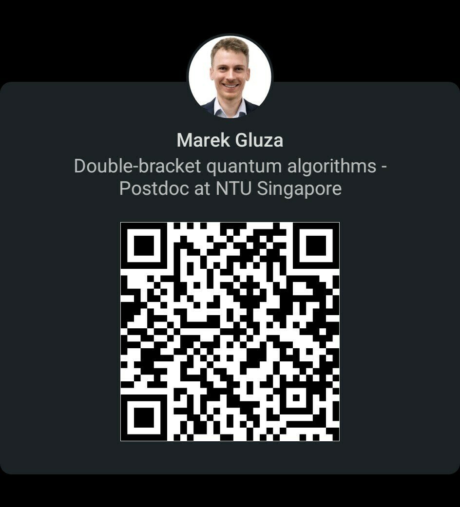
Marek Gluza
NTU Singapore
slides.com/marekgluza

New quantum algorithm for diagonalization
\hat H \mapsto \hat \mathcal H_\ell = \hat \mathcal U_\ell^\dagger \hat H \hat\mathcal U_\ell
\partial_\ell \hat \mathcal H_\ell = [[A(\hat \mathcal H_\ell),B(\hat \mathcal H_\ell)], \hat \mathcal H_\ell]
no qubit overheads
no controlled-unitaries
0
0
0
0
C
0
0
0
0
Simple
=
Easy
Doesn't spark joy :(
New quantum algorithm for diagonalization
\hat H \mapsto \hat \mathcal H_\ell = \hat \mathcal U_\ell^\dagger \hat H \hat\mathcal U_\ell
\partial_\ell \hat \mathcal H_\ell = [[A(\hat \mathcal H_\ell),B(\hat \mathcal H_\ell)], \hat \mathcal H_\ell]
building useful quantum algorithms
new approach to preparing useful states
building useful variational circuits
tons of fun maths in the appendix
no qubit overheads
no controlled-unitaries
0
0
0
0
New quantum algorithm for diagonalization
\hat H \mapsto \hat \mathcal H_\ell = \hat \mathcal U_\ell^\dagger \hat H \hat\mathcal U_\ell
\partial_\ell \hat \mathcal H_\ell = [[A(\hat \mathcal H_\ell),B(\hat \mathcal H_\ell)], \hat \mathcal H_\ell]
0
0
0
0
\hat V^{(\Delta)}_s(\hat J) = \prod_{\mu\in\{0,1\}^{\times L}} \hat Z_\mu e^{-i s \hat J/D} \hat Z_\mu
\hat V^\text{(GC)}_s(\hat J) = \hat V^{(\Delta)}_{\sqrt{2s}}(\hat J)^\dagger e^{i\sqrt{2s}\hat J}\hat V^{(\Delta)}_{\sqrt{2s}}(\hat J)e^{-i\sqrt{2s}\hat J}
\hat V_k = \hat V_{k-1}\hat V^\text{(GC)}_s(\hat J_{k-1})
\hat J_{k-1} = \hat V_{k-1}^\dagger \hat H \hat V_{k-1}
1) Dephasing
2) Group commutator
3) Frame shifting

New quantum algorithm for diagonalization
\hat H \mapsto \hat \mathcal H_\ell = \hat \mathcal U_\ell^\dagger \hat H \hat\mathcal U_\ell
\partial_\ell \hat \mathcal H_\ell = [[A(\hat \mathcal H_\ell),B(\hat \mathcal H_\ell)], \hat \mathcal H_\ell]
0
0
0
0
\hat V^{(\Delta)}_s(\hat J) = \prod_{\mu\in\{0,1\}^{\times L}} \hat Z_\mu e^{-i s \hat J/D} \hat Z_\mu
\hat V^\text{(GC)}_s(\hat J) = \hat V^{(\Delta)}_{\sqrt{2s}}(\hat J)^\dagger e^{i\sqrt{2s}\hat J}\hat V^{(\Delta)}_{\sqrt{2s}}(\hat J)e^{-i\sqrt{2s}\hat J}
\hat V_k = \hat V_{k-1}\hat V^\text{(GC)}_s(\hat J_{k-1})
\hat J_{k-1} = \hat V_{k-1}^\dagger \hat H \hat V_{k-1}
Why does it work?
What have
condensed-matter theorists
been up to in the 90's?
BTW: For the next 2 years I will be working on theory support for prof. Rainer Dumke as NTU PPF (super-conducting qubits, tomography zoo, proof-of-principle quantum algorithms...)
Research assistant "quantum engineer" positions available
(python, mathematica, Qiskit)
\hat H
\hat \mathcal H_\ell = \hat \mathcal U_\ell^\dagger \hat H \hat\mathcal U_\ell
\partial_\ell \hat \mathcal H_\ell = [\hat \mathcal W_\ell, \hat \mathcal H_\ell]
\hat \mathcal W_\ell = [\Delta(\hat \mathcal H_\ell),\sigma(\hat \mathcal H_\ell)]
\partial_\ell \|\sigma(\hat \mathcal H_\ell)\|_{\text{HS}}^2 = -2\|\hat \mathcal W_\ell\|_{\text{HS}}^2
\Delta(\hat \mathcal H_\ell)
\sigma(\hat \mathcal H_\ell)
Głazek-Wilson-Wegner flow
GWW flow equation
Flow duration
GWW flow unitary
Flowed Hamiltonian
Input Hamiltonian
\hat\mathcal U_\ell
\ell
Canonical bracket
GWW flow monotonicity
Restriction to off-diagonal
Restriction to diagonal
as a quantum algorithm
\hat H
\hat \mathcal H_\ell = \hat \mathcal U_\ell^\dagger \hat H \hat\mathcal U_\ell
\partial_\ell \hat \mathcal H_\ell = [\hat \mathcal W_\ell, \hat \mathcal H_\ell]
\hat \mathcal W_\ell = [\Delta(\hat \mathcal H_\ell),\sigma(\hat \mathcal H_\ell)]
\Delta(\hat \mathcal H_\ell)
\sigma(\hat \mathcal H_\ell)
Głazek-Wilson-Wegner flow
GWW flow equation
Flow duration
GWW flow unitary
Flowed Hamiltonian
Input Hamiltonian
\hat\mathcal U_\ell
\ell
Canonical bracket
GWW flow monotonicity
Restriction to off-diagonal
Restriction to diagonal
\hat H
\hat \mathcal H_\ell = \hat \mathcal U_\ell^\dagger \hat H \hat\mathcal U_\ell
\partial_\ell \hat \mathcal H_\ell = [\hat \mathcal W_\ell, \hat \mathcal H_\ell]
\hat \mathcal W_\ell = [\Delta(\hat \mathcal H_\ell),\sigma(\hat \mathcal H_\ell)]
\partial_\ell \|\sigma(\hat \mathcal H_\ell)\|_{\text{HS}}^2 = -2\|\hat \mathcal W_\ell\|_{\text{HS}}^2
\Delta(\hat \mathcal H_\ell)
\sigma(\hat \mathcal H_\ell)
Głazek-Wilson-Wegner flow
GWW flow equation
Flow duration
GWW flow unitary
Flowed Hamiltonian
Input Hamiltonian
\hat\mathcal U_\ell
\ell
Canonical bracket
GWW flow monotonicity
Restriction to off-diagonal
Restriction to diagonal
as a quantum algorithm
\hat \mathcal W_\ell = [\Delta(\hat \mathcal H_\ell),\sigma(\hat \mathcal H_\ell)]
\partial_\ell \|\sigma(\hat \mathcal H_\ell)\|_{\text{HS}}^2 = -2\|\hat \mathcal W_\ell\|_{\text{HS}}^2 \le 0
Głazek-Wilson-Wegner flow
GWW flow monotonicity
as a quantum algorithm
What's going on?
Double-bracket flow
Unitary
Satisfies a generalization of the Heisenberg equation
\hat \mathcal H_\ell = \hat \mathcal U_\ell^\dagger \hat H \hat\mathcal U_\ell
\partial_\ell \hat \mathcal H_\ell = [[A(\hat \mathcal H_\ell),B(\hat \mathcal H_\ell)], \hat \mathcal H_\ell]
\hat\mathcal U_\ell
GWW is a particular example
\partial_\ell \hat \mathcal H_\ell = [[\Delta(\hat \mathcal H_\ell),\sigma(\hat \mathcal H_\ell)], \hat \mathcal H_\ell]
transformation of
\hat H
\hat H_s = e^{s \hat W^{(Z)}} \hat H e^{-s \hat W^{(Z)}}
\hat W^{(Z)} = [\Delta^{(Z)}(\hat H), \hat H ],
\partial_s \|\sigma(\hat H_s)\|_{\text{HS}}^2 = -2\langle \hat W^{(Z)},\hat W\rangle_{\text{HS}}
\Delta^{(Z)}(\hat H) \text{ - diagonal}
Variational double-bracket flows
that are diagonalizing

\partial_\ell \|\sigma(\hat \mathcal H_\ell)\|_{\text{HS}}^2 = -2\|\hat \mathcal W_\ell\|_{\text{HS}}^2 \le 0
antihermitian
unitary
\left(i\hat H\right)^\dagger = -i \hat H
How to understand the continuous flow?
\hat H_1 = e^{s \hat W_1} \hat H e^{-s \hat W_1}
\hat W_1 = [\Delta(\hat H),\sigma(\hat H)]
\hat W_k = [\Delta(\hat H_{k-1}),\sigma(\hat H_{k-1})]
\hat H_k = e^{s \hat W_k} \hat H_{k-1} e^{-s \hat W_k}

\hat H_\text{TFIM} = \sum_{i=1}^{L-1}\hat X_i\hat X_{i+1}+\sum_{i=1}^L \hat Z_i
Piece-wise constant discretization
\hat W_k = [\Delta(\hat H_{k-1}),\sigma(\hat H_{k-1})]
\hat H_k = e^{s \hat W_k} \hat H e^{-s \hat W_k}
\text{If we want } U_\ell \text{ then set } s = \ell / N \text{ and } N\rightarrow \infty
\text{{\bf Prop.} This converges point-wise:}
\partial_\ell \hat \mathcal H_\ell = [\hat \mathcal W_\ell, \hat \mathcal H_\ell]
\hat \mathcal W_\ell = [\Delta(\hat \mathcal H_\ell),\sigma(\hat \mathcal H_\ell)]
Piece-wise constant discretization
Programming Singapore's quantum computers
Marek Gluza
Senior Research Fellow
Nanyang Technological University
What I do: Programming Singapore's quantum computers
Together we can: Operate Singapore's quantum computers
-
How to be successful in quantum computing?
-
What is the moonshot project of quantum computing?
-
How will we get there?
4 stages of creating quantum algorithms
Guidelines for using quantum computing
Stage 1: Think. What is the goal?
Important problems that are difficult yet doable.
Encode what we know in \(\vec{v}_{input}\).
Decode information from \(\vec{v}_{output}\).
Find effective heuristics to reduce the runtime of rotations \(R_k\)
Find rotations such that
\(\vec{v}_{output} \approx R_1 R_2 \ldots R_n \vec{v}_{input}\)
Stage 2: Design. How to encode task in quantum mechanics?
|\psi(\tau)\rangle = \frac{e^{-\tau H}|\psi\rangle}{\| e^{-\tau H}|\psi\rangle\|}
Stage 4: Run it.
What instructions to send?
Stage 3: Algorithm. How to find \(\vec{v}_{output}\)?
Guidelines for extracting utility from quantum computing
Stage 1: Think. What is the goal?
- Bridge between needs of humans and technological feasibility.
- Exchange domain expertise with industry partners.
- My work: General-purpose optimization solver in quantum computing based on non-Euclidean geometry.
- My expertise: Algorithms optimized for execution on leading prototypes.
Stage 4: Run it.
What instructions to send?
Stage 2: Design. How to encode task in quantum mechanics?
Stage 3: Algorithm. How to find \(\vec{v}_{output}\)?
My work: Geometrical construction of quantum algorithms
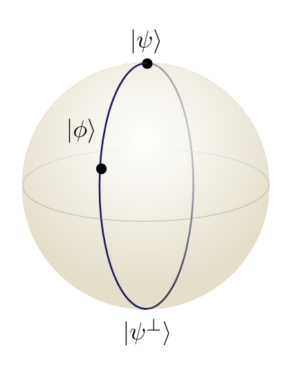
Mathematically, states of the quantum computer are like arrows pointing from the center of the sphere to its surface.
Observation leading to my algorithms: Earth is not flat. I.e., when we walk along of the equator, we think we are going straight but eventually we will wrap around it.
Fixing a direction and rotating the arrow, corresponds to a type of of quantum computing operation.
Stage 3: Algorithm. How to find \(\vec{v}_{output}\)?
On a flat surface DOWN-LEFT-UP-RIGHT will return to point of origin.
Stage 3: Algorithm. How to find \(\vec{v}_{output}\)?
My work: Geometrical construction of quantum algorithms
On a flat surface DOWN-LEFT-UP-RIGHT will return to point of origin.
On a curved surface SOUTH-WEST-NORTH-EAST will spiral way.
South
West
East
North
Stage 3: Algorithm. How to find \(\vec{v}_{output}\)?
My work: Geometrical construction of quantum algorithms
My work: New geometric guideline for quantum computing
South
West
East
North
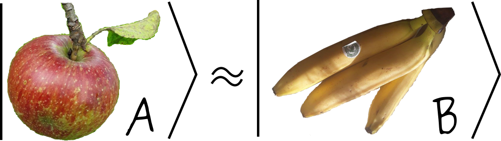
My invention, double-bracket quantum algorithms, shows how to use this spiraling effect to implement non-Euclidean gradient descent in quantum computing.
Regular machine learning fails for quantum computing but our generalization works. The 'failed' machine learning is still key for us - as a warm-start!

(Physical Review Letters '26)
Stage 3: Algorithm. How to find \(\vec{v}_{output}\)?
The Moonshot:
- Run double-bracket quantum algorithms on commercially available quantum computers to realize states of quantum materials that we cannot simulate numerically.
- Study their physics using a quantum computer, derive predictions, drive innovations.
Materials science?
Strategic Keystones:
- Industry Partnerships: Domain expertise (e.g. joint PhD with Thales Singapore)
- QC Hardware Providers: Existing collaboration network (e.g. NDA with Quantinuum in motion, collaborators at IQM)
- 3-tier quantum technology curriculum: University-wide offer to familiarize, use, and develop (Github homeworks, collaborators from India, Thailand, Kenya and South Africa)
Marek Gluza
My teaching and supervision approach:
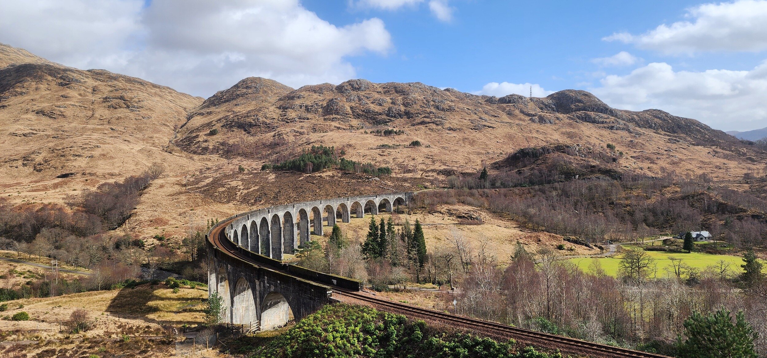
I grew up around these mountains where Poland meets Czech Republic and Slovakia (in Europe)
June '22: Single-author double-bracket proposal

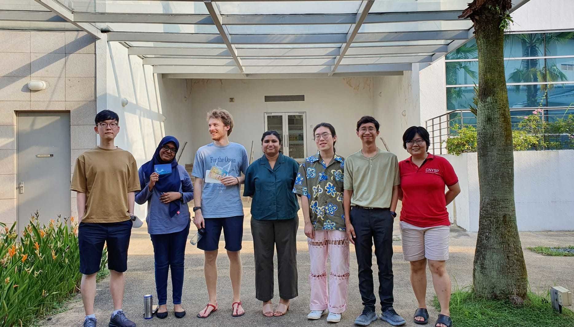
- As postdoc brought together collaboration of 25 co-authors \(\rightarrow\) Leadership skills
- Thanks to tutoring and lecturing experience \(\rightarrow\) Effective coaching younger peers (hired research assistants, supervised and evaluated FYP, BSc., MSc. projects; communication and clarity was key).
- Values guiding us \(\rightarrow\) Creativity is a sustainable intellectual drive! (And it's fun)

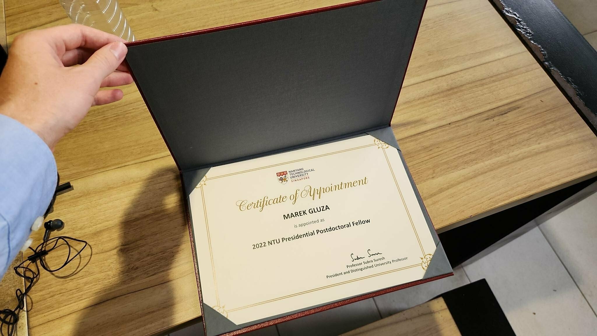
October '21: Arrived to Singapore
4 years of working on the real-deal in quantum computing:
The moonshot:
- Realize on commercially available hardware states of quantum materials that we cannot simulate numerically.
- Study their physics using a quantum computer, derive predictions, drive innovations.
- As a by-product pay attention to what we learned in the process.
Materials science?
Successful completion will come from:
- Domain expertise from industry (e.g. joint PhD with Thales Singapore)
- Work with top quantum computing hardware providers (e.g. NDA with Quantinuum in motion, collaborators at IQM)
- New curriculum (Github driven, collaborators from India, Thailand, Kenya and South Africa)
Let us choose to do quantum computing... not because it is easy, but because it is hard; because that goal will serve to organize and measure the best of our energies and skills.

Houston, we’re ready for take-off!
In summary:
Research is planned, team is in place and the time is right.
It's clear what to do and why it is important.
Itching to get going. All I need is "the spaceship" for the moonshot!
My roadmap:
Overarching fact: Quantum computing is not a one-man show.
Goal: Grow new quantum leaders.
Action: Horizontal & Github based quantum curriculum, with partner universities globally, internships with prospective clients and providers.
Current stage
Advanced stage
Intermediate stage
My roadmap:
Current stage
Advanced stage
Intermediate stage
Fact: Quantum computers are already quite powerful.
Goal: Creative hacking of their functionalities to get impact now.
Action: Lend tailored quantum algorithms to companies, R&D together.
Upcoming: Big quantum computers will be disruptive.
Goal: Thought leadership to utilize them with positive impact to our prosperity.
Action: Honest, grounded and diligent research on the real-deal.
Opportunity: Small quantum computers can be useful.
Goal: Use en-mass field-deployable quantum computing mindset for innovating MRIs, certifying thin-film deposition, etc.
Action: Evolve as physicist; think innovation first, revenue second.
Overarching fact: Quantum computing is not a one-man show.
Goal: Grow new quantum leaders.
Action: Horizontal & Github based quantum curriculum, with partner universities globally, internships with prospective clients and providers.
My roadmap:
Fact: Quantum computing is not a one-man show.
Goal: Grow new quantum leaders.
Action: Horizontal & Github based quantum curriculum, with partner universities globally, internships with prospective clients and providers.
Fact: Quantum computers are already quite powerful.
Goal: Creative hacking of their functionalities to get impact now.
Action: Lend tailored quantum algorithms to companies, R&D together.
Upcoming: Big quantum computers will be disruptive.
Goal: Thought leadership to utilize them with positive impact to our prosperity.
Action: Honest, grounded and diligent research on the real-deal.
Opportunity: Small quantum computers can be useful.
Goal: Use en-mass field-deployable quantum computing mindset for innovating MRIs, certifying thin-film deposition, etc.
Action: Evolve as physicist; think innovation first, revenue second.
Quantum algorithmic protocols for extracting properties of materials
Marek Gluza
Nanyang Assistant Professor
Nanyang Technological University
Marek Gluza
My journey:
I grew up around these mountains where Poland meets Czech Republic and Slovakia (in Europe)
June '22: Single-author double-bracket proposal
- As postdoc brought together collaboration of 25 co-authors on [1-9], 37 co-authors on [1-14]! \(\rightarrow\) Leadership skills
- Thanks to tutoring and lecturing experience \(\rightarrow\) Effectively coaching younger peers
- Values guiding us \(\rightarrow\) Creativity is a sustainable intellectual drive! (And it's fun)
Successful research program:
[10-14] In prep.
October '21: Arrived to Singapore
4 years of working on the real-deal in quantum computing:
March '26: Started NAP
Why would a quantum computing guy be showing you jetfighters?
Vision: Use quantum computers as an economically viable filter helping to select the one-in-a-million stoichiometric ratio
Characterization bottleneck:
- It is easy to fabricate many samples of materials with different compositions
- A 'human' lab can test only few of them
- How do you select the best one?
What do I mean by 'the best' stoichiometric ratio?
Optimize properties like:
- Charge mobility
- Specific heat
- Density of states
- Structure factor
Leadership position in using quantum hardware for condensed-matter and solid state physics studies
What do I mean by 'the best' stoichiometric ratio?
Optimize properties like:
- Charge mobility
- Specific heat
- Density of states
- Structure factor
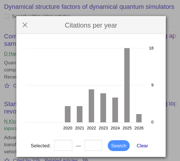
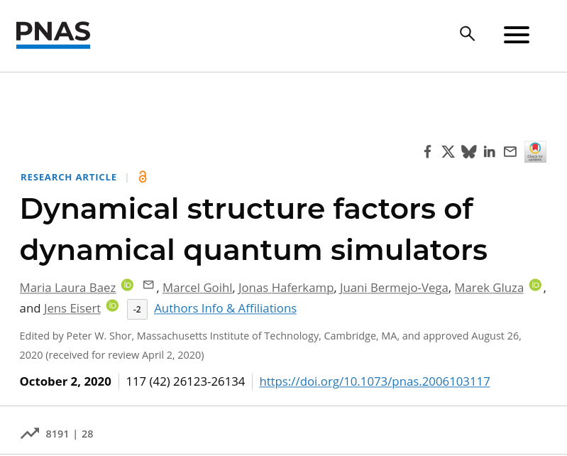
50 citations even though we all moved to other topics
Next:
- Three challenges ahead
- Proposal how to solve them
- Summary
How do we make a quantum computer talk about a material?
How do we account for failures of a quantum computing prototype?
How do we increase our understanding of material?
The Nanyang Quantum Solutions group sets out to serve as the bridge between the quantum software and hardware, between technological capacities and civilizational needs.
How do we make a quantum computer talk about a material?
We need to prepare a quantum state representing low-energy physics of the material.
Low-energy landscape is barren and computationally hard.
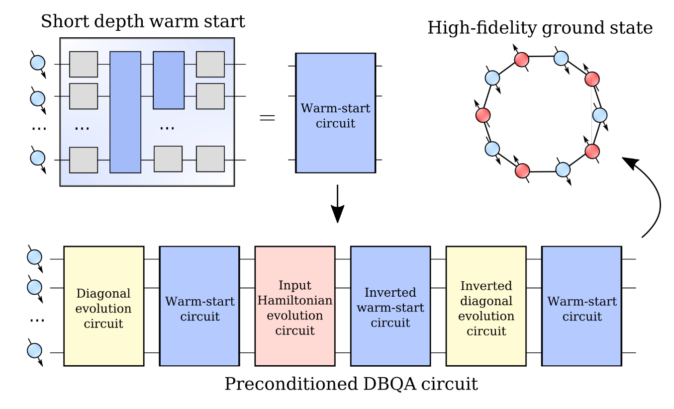
We outperform state-of-the-art and benefit from machine learning warm-starts, an approach which alone failed due to the barren plateau phenomenon.
(Physical Review Letters '26)
Work-package 1:
Enable reaching sufficiently low energies on a quantum computer to emulate physics of materials.
3 deliverables:
- Optimized circuit compilation
- Nesterov acceleration in q. computing
- New DBQAs for effective models
My work established double-bracket quantum algorithms as a leading solution for preparing low-energy states of quantum many-body systems.
How do we increase our understanding of material?
Work-package 2: Provide predictions for precise linear-response functions expected from quantum computations and demonstrate readiness
Deliverable A: Quantitative selection guidelines for unequal-time correlation measurement methods
Deliverable B: Guide for quantum computing experts which response function to study
Deliverable C: Demonstrate readiness of quantum hardware to guide material discovery
WP2-A: Add more!
WP2-B: 2d numerics
WP2-C: 9x9 q. computations
S. Thomson, Edinburgh
NQO collaboration with Quantinuum
How to disentangle from depending on quantum computing prototypes?
Does the success of this research rest on waiting for better hardware?
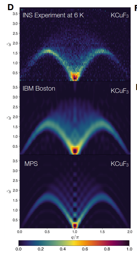
Deliverable A. It is already good: "IBM Heron outputs in 10 mins what my tensor networks does in 1 week on a cluster." Show that existing hardware has faster time-to-solution runtime for DSF.
Work-package 3: Map-out robustness of linear-response functions allowing to prioritize focus points for error mitigation.
Deliverable B. Ask a physicist: Response functions are 'nice' observables. Previous reports of evolution simulation robustness, our PNAS was first for DSF. Broadcast this!
Deliverable C. No need for qubits: Materials science is about fermions. DBQAs can program fermionic quantum computers.
P. Preiss
MPQ Munich
Summary & next steps:
Vision: Develop specialized quantum computations of linear-response functions to help filter which compositions of materials are advantageous.
Timely: I have leadership position in this field, and it will only grow in importance.
Feasible: Not just develop quantum computers but use them!
Work-package 2: Materials applications
S. Thomson, Edinburgh


Work-package 1: State preparation
Work-package 3: Quantum hardware


R. Seidel, IQM
S. Thanasilp,
Chulalongkorn, Thailand
F. Barbaresco, Thales
C. Mostajeran,
NTU
N. Ng,
NTU
Y. Suzuki,
EPFL
Z. Holmes, EPFL, Algorithmiq
C. Arenz,
Arizona S. U.
R. Zander,
Fraunhofer
Berlin
T. Silva,
TII Abu Dhabi
S. Carrazza, CERN
TS. Mahesh
IISER Pune
P. Preiss
MPQ Munich
J. Schmiedmayer,
TU Wien
R. Dumke,
NTU Singapore
D. Wilkowski,
NTU Singapore
On the first workshop that I attended, as a Masters student, I heard Matthias Troyer open his talk saying: "I want to work with the best computers. So I have to work with quantum computers".
10 years later, what are the things we can compute with these computers?
Through this funding:
- I will show how to extract properties of materials using quantum computers. That means we physicists will be their first users.
- We program quantum computers by prescribing which forces to switch on and for how long. That's my expertise: I invented double-bracket quantum algorithms and have led the effort to establish them as a general purpose optimization solver.
Double-bracket quantum algorithms
- Coherently implement Riemannian gradient steps
-
Give rigorous unitary synthesis for
- imaginary-time evolution
- quantum signal processing
- diagonalization unitaries
- Grover's as an approximation to imaginary-time evolution
- Training quantum circuits from data doesn't work well, unlike in classical machine learning applications. However those variational learning methods are great for warm-starting double-bracket quantum algorithms!

Tell me when not fast enough? Get stuck? Something else?
Your input is needed to improve them!
N. Ng
Z. Holmes
R. Zander
R. Seidel
Y. Suzuki
B. Tiang
J. Son
S. Carrazza
Stay in touch on LinkedIn:
Text
Text
Text
Group commutator
\hat H \mapsto \hat \mathcal H_\ell = \hat \mathcal U_\ell^\dagger \hat H \hat\mathcal U_\ell
\partial_\ell \hat \mathcal H_\ell = [[A(\hat \mathcal H_\ell),B(\hat \mathcal H_\ell)], \hat \mathcal H_\ell]
0
0
0
0
Want
\hat H_1 = e^{s \hat W_1} \hat H e^{-s \hat W_1}
\hat W_1 = [\Delta(\hat H),\sigma(\hat H)]
e^{is\Delta(\hat H)}e^{is\hat H}e^{-is\Delta(\hat H)}e^{-is\hat H}= e^{-\frac12 s^2[\Delta(\hat H),\sigma(\hat H)]} +\hat E^\text{(GC)}
New bound
\|\hat E^\text{(GC)}\| \le 4\|\hat H\|\,\|[\Delta(\hat H),\sigma(\hat H)]\| s^3
Group commutator
\hat H \mapsto \hat \mathcal H_\ell = \hat \mathcal U_\ell^\dagger \hat H \hat\mathcal U_\ell
\partial_\ell \hat \mathcal H_\ell = [[A(\hat \mathcal H_\ell),B(\hat \mathcal H_\ell)], \hat \mathcal H_\ell]
0
0
0
0
Want
\hat H_1 = e^{s \hat W_1} \hat H e^{-s \hat W_1}
\hat W_1 = [\Delta(\hat H),\sigma(\hat H)]
e^{is\Delta(\hat H)}e^{is\hat H}e^{-is\Delta(\hat H)}e^{-is\hat H}= e^{-\frac12 s^2[\Delta(\hat H),\sigma(\hat H)]} +\hat E^\text{(GC)}
How to get ?
\hat V^{(\Delta)}_s(\hat H) \approx e^{is\Delta(\hat H)}
\hat V^\text{(GC)}_s(\hat J) = \hat V^{(\Delta)}_{\sqrt{2s}}(\hat J)^\dagger e^{i\sqrt{2s}\hat J}\hat V^{(\Delta)}_{\sqrt{2s}}(\hat J)e^{-i\sqrt{2s}\hat J}
\approx e^{-s \hat W(\hat J)}
New quantum algorithm for diagonalization
\hat H \mapsto \hat \mathcal H_\ell = \hat \mathcal U_\ell^\dagger \hat H \hat\mathcal U_\ell
\partial_\ell \hat \mathcal H_\ell = [[A(\hat \mathcal H_\ell),B(\hat \mathcal H_\ell)], \hat \mathcal H_\ell]
0
0
0
0
\hat V^{(\Delta)}_s(\hat J) = \prod_{\mu\in\{0,1\}^{\times L}} \hat Z_\mu e^{-i s \hat J/D} \hat Z_\mu
\hat V^\text{(GC)}_s(\hat J) = \hat V^{(\Delta)}_{\sqrt{2s}}(\hat J)^\dagger e^{i\sqrt{2s}\hat J}\hat V^{(\Delta)}_{\sqrt{2s}}(\hat J)e^{-i\sqrt{2s}\hat J}
\hat V_k = \hat V_{k-1}\hat V^\text{(GC)}_s(\hat J_{k-1})
\hat J_{k-1} = \hat V_{k-1}^\dagger \hat H \hat V_{k-1}
1) Dephasing
2) Group commutator
3) Frame shifting
\hat H
\hat \mathcal H_\ell = \hat \mathcal U_\ell^\dagger \hat H \hat\mathcal U_\ell
\partial_\ell \hat \mathcal H_\ell = [\hat \mathcal W_\ell, \hat \mathcal H_\ell]
\hat \mathcal W_\ell = [\Delta(\hat \mathcal H_\ell),\sigma(\hat \mathcal H_\ell)]
\partial_\ell \|\sigma(\hat \mathcal H_\ell)\|_{\text{HS}}^2 = -2\|\sigma(\hat \mathcal W_\ell)\|_{\text{HS}}^2
\Delta(\hat \mathcal H_\ell)
\sigma(\hat \mathcal H_\ell)
Głazek-Wilson-Wegner flow
GWW flow equation
Flow duration
GWW flow unitary
Flowed Hamiltonian
Input Hamiltonian
\hat\mathcal U_\ell
\ell
Canonical bracket
GWW flow monotonicity
Restriction to off-diagonal
Restriction to diagonal
Dephasing is a unitary mixing channel:
\Delta(\hat \mathcal H_\ell)= \frac 1 D \sum_{\mu\in\{0,1\}} \hat Z_\mu \hat\mathcal H_\ell \hat Z_\mu
as a quantum algorithm
1,
1,
1,
1,
0,
0,
0,
0
What I mean by phase flips
\mu = (
)
N
S
N
S
N
S
N
S
\hat Z
\mathbb 1
\mathbb 1
\otimes
\otimes
\otimes
\otimes
\otimes
\otimes
\otimes
\hat Z
\hat Z
\hat Z
\mathbb 1
\mathbb 1
0,
1,
0,
1,
0,
0,
0,
1
What I mean by phase flips
\mu = (
)
1
\otimes
\mathbb 1
\otimes
\mathbb 1
\otimes
\hat Z
\otimes
1
\otimes
\mathbb 1
\otimes
\hat Z
\otimes
\hat Z
N
S
N
S
N
S
Evolution under dephased generators
\hat H \mapsto \hat \mathcal H_\ell = \hat \mathcal U_\ell^\dagger \hat H \hat\mathcal U_\ell
\partial_\ell \hat \mathcal H_\ell = [[A(\hat \mathcal H_\ell),B(\hat \mathcal H_\ell)], \hat \mathcal H_\ell]
0
0
0
0
e^{-is/D \sum_{\mu\in\{0,1\}^{\times L}} \hat Z_\mu \hat J\hat Z_\mu} \approx \prod_{\mu\in\{0,1\}^{\times L}} \hat Z_\mu e^{-i s \hat J/D} \hat Z_\mu
\hat V^{(\Delta)}_s(\hat J) \approx \prod_{\mu\in R} \hat Z_\mu e^{-i s \hat J/D} \hat Z_\mu
Can we make it efficient?
\Delta(\hat \mathcal H_\ell)= \frac 1 D \sum_{\mu\in\{0,1\}} \hat Z_\mu \hat\mathcal H_\ell \hat Z_\mu
R \subseteq \{0,1\}^{\times L}
New quantum algorithm for diagonalization
\hat H \mapsto \hat \mathcal H_\ell = \hat \mathcal U_\ell^\dagger \hat H \hat\mathcal U_\ell
\partial_\ell \hat \mathcal H_\ell = [[A(\hat \mathcal H_\ell),B(\hat \mathcal H_\ell)], \hat \mathcal H_\ell]
0
0
0
0
\hat V^{(\Delta)}_s(\hat J) = \prod_{\mu\in\{0,1\}^{\times L}} \hat Z_\mu e^{-i s \hat J/D} \hat Z_\mu
\hat V^\text{(GC)}_s(\hat J) = \hat V^{(\Delta)}_{\sqrt{2s}}(\hat J)^\dagger e^{i\sqrt{2s}\hat J}\hat V^{(\Delta)}_{\sqrt{2s}}(\hat J)e^{-i\sqrt{2s}\hat J}
\hat V_k = \hat V_{k-1}\hat V^\text{(GC)}_s(\hat J_{k-1})
\hat J_{k-1} = \hat V_{k-1}^\dagger \hat H \hat V_{k-1}
1) Dephasing
2) Group commutator
3) Frame shifting
How well does it work?

Variational flow example
Notice the steady increase of diagonal dominance.


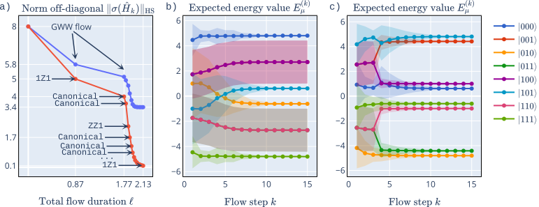
Variational vs. GWW flow
Notice that degeneracies limit GWW diagonalization but variational brackets can lift them.

GWW for 9 qubits
Notice the spectrum is almost converged.


GWW for 9 qubits
Notice that some of them are essentially eigenstates!
Runtime
- are you running the full scheme or heuristics?
\text{{\bf Prop.} The prescription converges to GWW } \\ \|\hat V_N -\hat \mathcal U_\ell\|\le O\left(e^{16 \|\hat H\|^2\ell} \sqrt{\frac \ell N}\right)
- number of queries assuming worst-case
\mathcal N(N) \sim 2^{N L}
Runtime
- are you running heuristics?
1) Not
s = \ell / N
s_1,\ldots, s_N
but optimize durations

2) It's not necessary to Hamiltonian simulate
e^{-s\hat W}
3) It's possible to Hamiltonian simulate
\hat V^\text{(pGGW)} = e^{-s_1 \hat W_1}\ldots e^{-s_5 \hat W_5}
4) Use approximate dephasing
5) Use variational brackets
Each of these reduces the runtime
\mathcal N(N) \sim poly(N) exp(L)
\mathcal N(N) \sim poly(N,L)
How does it work again?
New quantum algorithm for diagonalization
\hat H \mapsto \hat \mathcal H_\ell = \hat \mathcal U_\ell^\dagger \hat H \hat\mathcal U_\ell
\partial_\ell \hat \mathcal H_\ell = [[A(\hat \mathcal H_\ell),B(\hat \mathcal H_\ell)], \hat \mathcal H_\ell]
0
0
0
0
\hat V^{(\Delta)}_s(\hat J) = \prod_{\mu\in\{0,1\}^{\times L}} \hat Z_\mu e^{-i s \hat J/D} \hat Z_\mu
\hat V^\text{(GC)}_s(\hat J) = \hat V^{(\Delta)}_{\sqrt{2s}}(\hat J)^\dagger\; e^{i\sqrt{2s}\hat J}\;\hat V^{(\Delta)}_{\sqrt{2s}}(\hat J)\;e^{-i\sqrt{2s}\hat J}
\hat V_k = \hat V_{k-1}\hat V^\text{(GC)}_s(\hat J_{k-1})
\hat J_{k-1} = \hat V_{k-1}^\dagger \hat H \hat V_{k-1}
1) Dephasing
2) Group commutator
3) Frame shifting
What else is there?
Linear programming
Matching optimization
Diagonalization
Sorting
QR decomposition
Toda flow
Are we done?
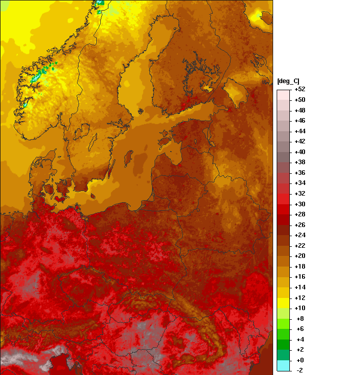
Short weather forecast
Heat waves destroy forests.
Heat waves destroy quantum computations.
0
0
0
0
C
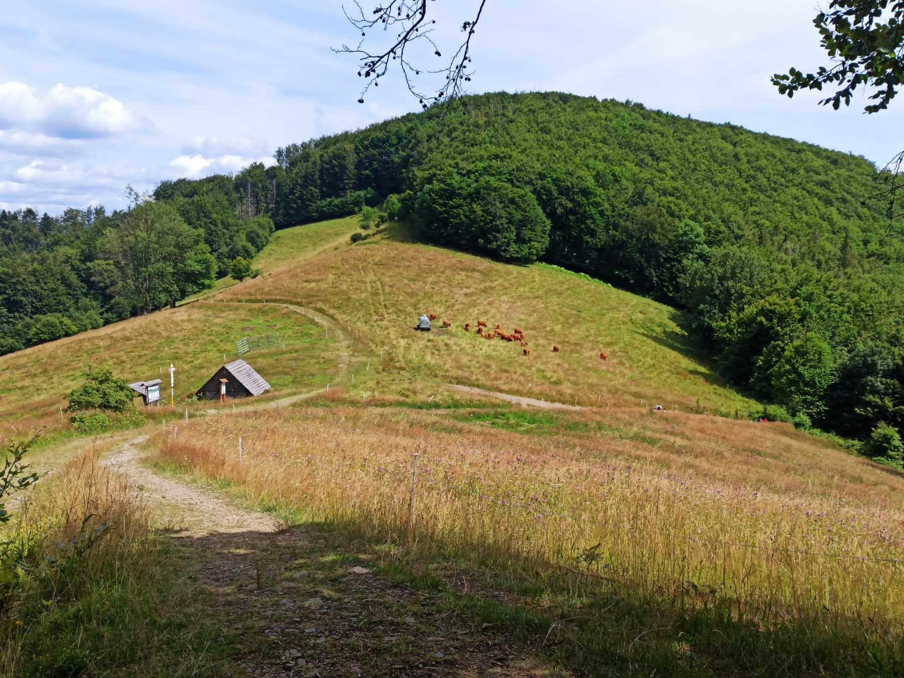
From where I come from, I can tell you:
Winter can be very beautiful!
But, I can also tell you: You get sad from the darkness, annoyed from the moisture and restricted by the cold.
Quantum winter
Quantum computers
Useful tasks?
If for
No
Then
BUT!

Quantum winter
Quantum computers
Useful tasks!
If for
No
Then
Material science?
0
0
0
0
C


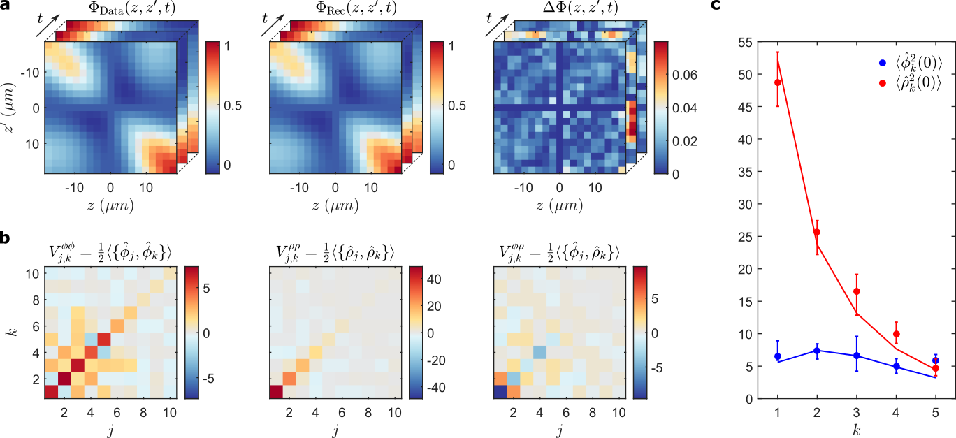
\langle\hat \phi_k^2(t)\rangle= \cos^2(\omega_k t) \langle \phi_k^2(0)\rangle \\
\quad\quad\quad\quad\quad+\sin^2(\omega_k t) \langle \delta\hat \rho_k^2(0)\rangle

\delta \hat\rho
\langle\hat \phi^2(t)\rangle
\langle\delta\hat \rho^2(0)\rangle =0?
\langle \hat \phi^2(0)\rangle
\hat \phi
Ask me anytime:
[4,8]
[1]

[3]
[2]
[5]
[13]

[6]

[9]
[11,16]
[12]
[7, 14, 15, 17]
[10]

0
0
0
0
C
Fidelity witnesses
Tomography optical lattices
Tomography phonons
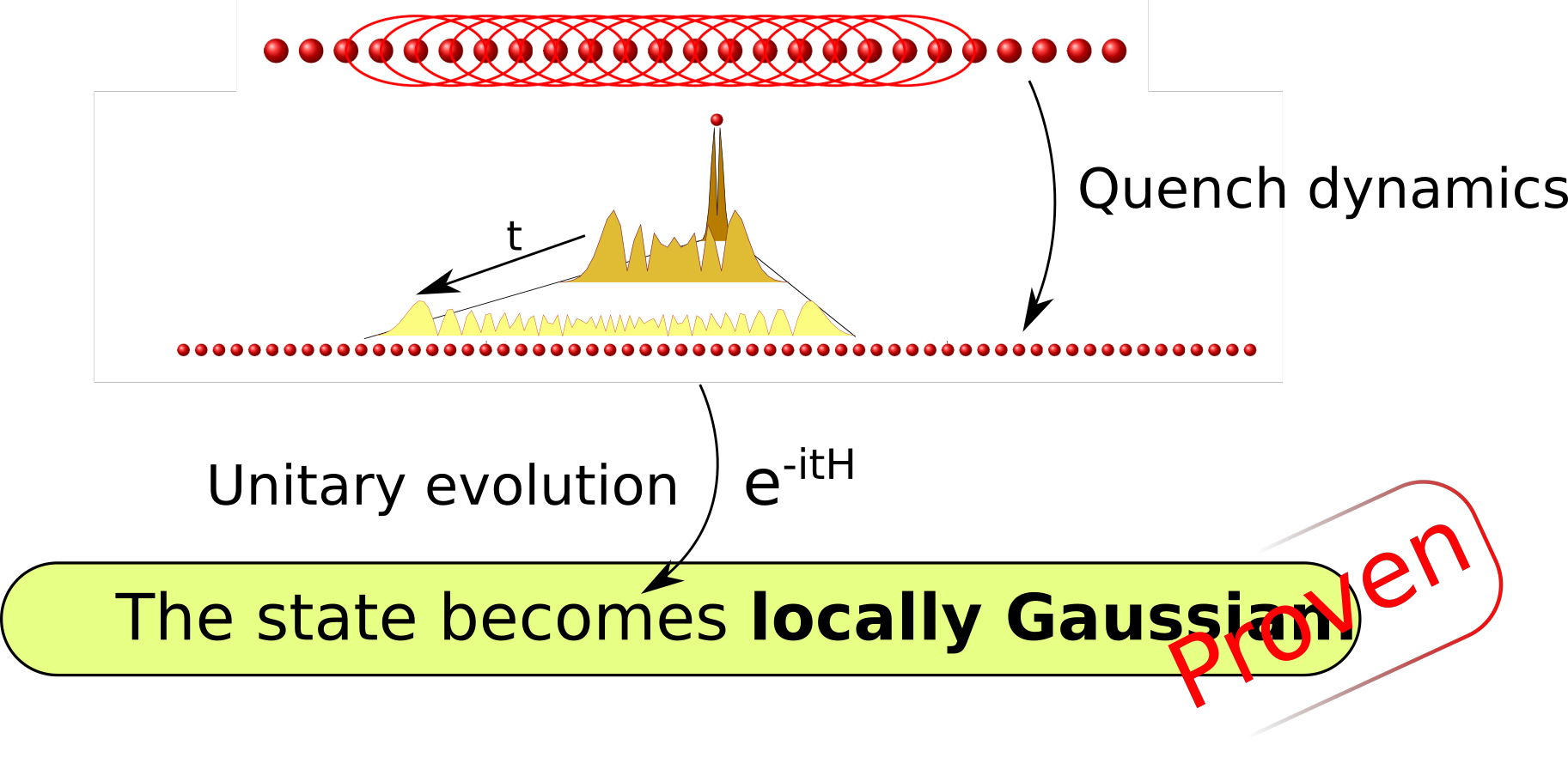
Proving statistical mechanics
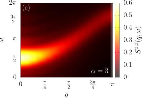
Quantum simulating DSF
Holography in tensor networks
PEPS contraction average #P-hard
Quantum field machine
MBL l-bits
\langle\hat \phi_k^2(t)\rangle= \cos^2(\omega_k t) \langle \phi_k^2(0)\rangle \\
\quad\quad\quad\quad\quad+\sin^2(\omega_k t) \langle \delta\hat \rho_k^2(0)\rangle
\delta \hat\rho
\langle\hat \phi^2(t)\rangle
\langle\delta\hat \rho^2(0)\rangle =0?
\langle \hat \phi^2(0)\rangle
\hat \phi
My background
0
0
0
0
C
[4,8]
[1]
[3]
[2]
[5]
[13]
[6]
[9]
[11,16]
[12]
[7, 14, 15, 17]
[10]
|\psi(t)\rangle = e^{-it \hat H}|\psi(0)\rangle
How to compute it on a laptop?
How to compute it on a quantum computer?
Hamiltonian simulation
|\psi(t)\rangle = e^{-it \hat H}|\psi(0)\rangle
How to compute it on a quantum computer?
Use quantum algorithms 'Hamiltonian simulation'
Trotter-Suzuki
Linear combination of unitaries
Qubitization
Randomized compiler
Hamiltonian simulation
Gaussian quantum simulators

Trotter-Suzuki decomposition
\|\hat E\| = \|e^{-it(\hat H_X +\hat H_Z)} - \left(e^{-i\frac tN \hat H_X}e^{-i\frac tN \hat H_Z}\right)^N\|
\le \frac{t^2}N\|[\hat H_X,\hat H_Z]\|
Why does it work?
BCH formula
e^{-it( \hat H_X +\hat H_Z)}=e^{-it\hat H_X }e^{-it\hat H_Z}e^{-i\frac {t^2}2[\hat H_X ,\hat H_Z]}\ldots
\|\mathbb 1 - e^{-i\frac {t^2}2[\hat H_X ,\hat H_Z]}\| \le \frac {t^2}2 \|[ \hat H_X ,\hat H_Z]\|
Conclusion: For short evolution time we're happy
How to implement Trotter-Suzuki?
e^{-it\hat H_X}=\prod_{i=1}^{L-1}e^{-it X_iX_{i+1} }
g_X(i) = e^{-itX_i X_{i+1}}
g_Z(i) = e^{-itZ_i }
Use Solovay-Kitaev algorithm to compile these gates but usually they are the primitive gates
(e^{-i\frac tN \hat H_X}e^{-i\frac tN \hat H_Z})^N{|0\rangle}^{\otimes L}
0
0
0
0
Hamiltonian simulation
0
0
0
0
0
0
0
0
C

Most sophisticated theoretical methods use
controlled-unitary operations
Exercise: Local error bound
Q_x = e^{i(1-x)A}e^{i(1-x)B}e^{ix(A+B)}
Q_1 = e^{i(A+B)}
Q_0 = e^{i A}e^{i B}
\partial_x Q_x = e^{i(1-x)A}\left(-A-B+ A_B+B\right)e^{i(1-x)B} e^{ix(A+B)}
A_B = e^{i(1-x)B}A e^{-i(1-x)B} = A + i e^{i\xi_x B}[A,B] e^{-i\xi_x B}
\|Q_0-Q_1\| =\| \int_0^1 dx \partial_x Q_x\| = \|[A,B]\|
Exercise: Non-commutative identity
X^m - Y^m = \sum_{j=0}^{m-1}X^{m-1-j}(X-Y)Y^j
\le \sum_{j=0}^{N-1}\|e^{-i (N-1-j)\frac tN \hat H_X}(e^{-i\frac tN \hat H_X}-e^{-i\frac tN \hat H_Z})e^{-ij\frac tN \hat H_Z}\|
\|e^{-it(\hat H_X +\hat H_Z)} - \left(e^{-i\frac tN \hat H_X}e^{-i\frac tN \hat H_Z}\right)^N\|
\le \sum_{j=0}^{N-1}\|e^{-i \frac tN \hat H_X}-e^{-i\frac tN \hat H_Z}\| \le \frac{t^2}N \|[H_X,H_Z]\|
cf.:
x^m -y ^m = (x-y)\sum_{j=0}^{m-1}x^{m-1-j}y^j
Application to physics:
dsf
By Marek Gluza


