Lecture:
Quantum
simulation
Marek Gluza
NTU Singapore
slides.com/marekgluza

|\psi(t)\rangle = e^{-it \hat H}|\psi(0)\rangle
How to compute it on a laptop?
How to compute it on a quantum computer?
Hamiltonian simulation
|\psi(t)\rangle = e^{-it \hat H}|\psi(0)\rangle
How to compute it on a laptop?
For qubits, your laptop can do ~13 spins at finite temperature and ~25 spins for a pure state (use sparsity)
\begin{pmatrix}1\\0\end{pmatrix}\otimes \begin{pmatrix}1\\0\end{pmatrix} = \begin{pmatrix}1\\0\\0\\0\end{pmatrix}
At the end of the day:
Workarounds:
Hamiltonian simulation
|\psi(t)\rangle = e^{-it \hat H}|\psi(0)\rangle
How to compute it on a quantum computer?
Use quantum algorithms 'Hamiltonian simulation'
Trotter-Suzuki
Linear combination of unitaries
Qubitization
Randomized compiler
Hamiltonian simulation
Truncated series

P: Runs easily
BPP: Often runs easily
BQP: Often quantums easily
NP: Optimizes easily
QMA
P: Runs easily
BPP: Often runs easily
BQP: Often quantums easily
NP: Optimizes easily
Trotter-Suzuki decomposition
\hat H_\text{TFIM} = \sum_{i=1}^{L-1}X_iX_{i+1}+\sum_{i=1}^L Z_i
\equiv \hat H_X +\hat H_Z
|\psi(t)\rangle = e^{-it \hat H_\text{TFIM}}{|0\rangle}^{\otimes L}
|\psi(t)\rangle = \left(e^{-i\frac tN \hat H_X}e^{-i\frac tN \hat H_Z}\right)^N{|0\rangle}^{\otimes L} + \hat E{|0\rangle}^{\otimes L}
Trotter-Suzuki decomposition
\|\hat E\| = \|e^{-it(\hat H_X +\hat H_Z)} - \left(e^{-i\frac tN \hat H_X}e^{-i\frac tN \hat H_Z}\right)^N\|
\le \frac{t^2}N\|[\hat H_X,\hat H_Z]\|
Why does it work?
BCH formula
e^{-it( \hat H_X +\hat H_Z)}=e^{-it\hat H_X }e^{-it\hat H_Z}e^{-i\frac {t^2}2[\hat H_X ,\hat H_Z]}\ldots
\|\mathbb 1 - e^{-i\frac {t^2}2[\hat H_X ,\hat H_Z]}\| \le \frac {t^2}2 \|[ \hat H_X ,\hat H_Z]\|
Conclusion: For short evolution time we're happy
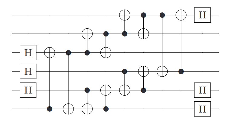
How to implement Trotter-Suzuki?
e^{-it\hat H_X}=\prod_{i=1}^{L-1}e^{-it X_iX_{i+1} }
g_X(i) = e^{-itX_i X_{i+1}}
g_Z(i) = e^{-itZ_i }
Use Solovay-Kitaev algorithm to compile these gates but usually they are the primitive gates
(e^{-i\frac tN \hat H_X}e^{-i\frac tN \hat H_Z})^N{|0\rangle}^{\otimes L}
0
0
0
0
Hamiltonian simulation
0
0
0
0
0
0
0
0
C
Most sophisticated theoretical methods use
controlled-unitary operations
Exercise: Local error bound
Q_x = e^{i(1-x)A}e^{i(1-x)B}e^{ix(A+B)}
Q_1 = e^{i(A+B)}
Q_0 = e^{i A}e^{i B}
\partial_x Q_x = e^{i(1-x)A}\left(-A-B+ A_B+B\right)e^{i(1-x)B} e^{ix(A+B)}
A_B = e^{i(1-x)B}A e^{-i(1-x)B} = A + i e^{i\xi_x B}[A,B] e^{-i\xi_x B}
\|Q_0-Q_1\| =\| \int_0^1 dx \partial_x Q_x\| = \|[A,B]\|
Exercise: Non-commutative identity
X^m - Y^m = \sum_{j=0}^{m-1}X^{m-1-j}(X-Y)Y^j
\le \sum_{j=0}^{N-1}\|e^{-i (N-1-j)\frac tN \hat H_X}(e^{-i\frac tN \hat H_X}-e^{-i\frac tN \hat H_Z})e^{-ij\frac tN \hat H_Z}\|
\|e^{-it(\hat H_X +\hat H_Z)} - \left(e^{-i\frac tN \hat H_X}e^{-i\frac tN \hat H_Z}\right)^N\|
\le \sum_{j=0}^{N-1}\|e^{-i \frac tN \hat H_X}-e^{-i\frac tN \hat H_Z}\| \le \frac{t^2}N \|[H_X,H_Z]\|
cf.:
x^m -y ^m = (x-y)\sum_{j=0}^{m-1}x^{m-1-j}y^j
Application to physics:
Key idea for post-Trotter methods
C(U,V) = |0\rangle\langle 0| \otimes U + |1\rangle\langle 1| \otimes V
Step 1: Show that it's unitary
C(U,V) \, C(U,V)^\dagger = |0\rangle\langle 0| \otimes UU^\dagger + |1\rangle\langle 1| \otimes V V^\dagger = \mathbb 1
Key idea for post-Trotter methods
C(U,V) = |0\rangle\langle 0| \otimes U + |1\rangle\langle 1| \otimes V
Step 2: Apply to flag qubit in superposition
C(U,V) (|0\rangle + |1\rangle) \otimes |\psi\rangle = |0\rangle \otimes U |\psi\rangle + |1\rangle \otimes V |\psi\rangle
Key idea for post-Trotter methods
C(U,V) = |0\rangle\langle 0| \otimes U + |1\rangle\langle 1| \otimes V
Step 3: Consider what happens if applied to superposition:
(R_x(\theta)\otimes 1)C(U,V) |+\rangle \otimes |\psi\rangle =
R_x(\theta) |0\rangle = c |0\rangle+ s |1\rangle
R_x(\theta) |1\rangle = c |1\rangle -s |0\rangle
|0\rangle \otimes (cU -s V) |\psi\rangle + |1\rangle \otimes (cV +sU) |\psi\rangle
Key idea for post-Trotter methods
C(U,V) = |0\rangle\langle 0| \otimes U + |1\rangle\langle 1| \otimes V
Step 4: Assume flag is measured with outcome 1 and discard it
(P_+\otimes 1)(R_x(\theta)\otimes 1)C(U,V) |+\rangle \otimes |\psi\rangle \propto (cU+s V) |\psi\rangle
R_x(\theta) |0\rangle = c |0\rangle+ s |1\rangle
R_x(\theta) |1\rangle = c |1\rangle -s |0\rangle
Conclusion: We can (probabilistically) apply (normalized) sums of unitary operators
Key idea for reliable post-Trotter methods
R = 1 - 2|\phi\rangle\langle \phi|
Grover reflector
Step 1: Show that it's unitary
...
Key idea for reliable post-Trotter methods
R = 1 - 2|\phi\rangle\langle \phi|
Grover reflector
Step 2: Consider applying it to a state overlapping with it
R(|\phi\rangle + |\phi^\perp\rangle) \propto - |\phi\rangle+ |\phi^\perp\rangle
Key idea for reliable post-Trotter methods
R = 1 - 2|\phi\rangle\langle \phi|
Grover reflector
Step 3: Reflect around the linear combination of unitaries
This is also called oblivious amplitude amplification, and the crux is in making this efficiently and obliviously i.e. without knowing or destroying the reflector state
R_{c,s} = Q(1-2|\phi\rangle\langle \phi|)Q^\dagger
Gaussian quantum simulators


How?

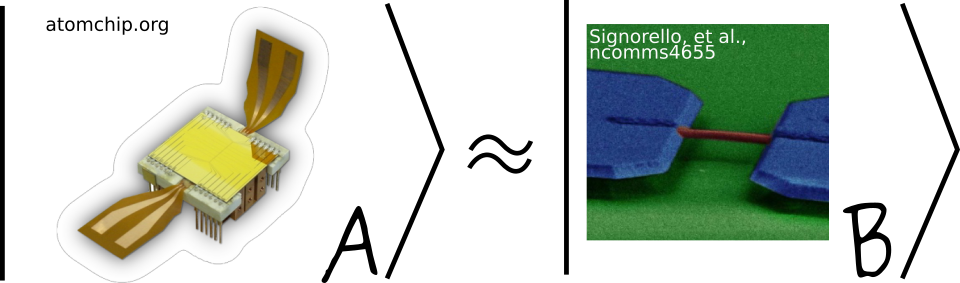
Ultra-cold 1d gases
Inside: atoms
Outside: wavepackets
hydrodynamics

Energy of phonons


E
E
E
E

\hat H_\text{TLL} = \int \text{d}z\left[ \frac{\hbar^2n_{GP}}{2m}\partial_z\hat\varphi^2+g\delta\hat\varrho^2\right]
\delta\varrho
\partial_z\varphi
\partial_z\varphi
\ll
\delta\varrho
\ll
Tomonaga-Luttinger liquid
Quantum field refrigerators in the TLL model:
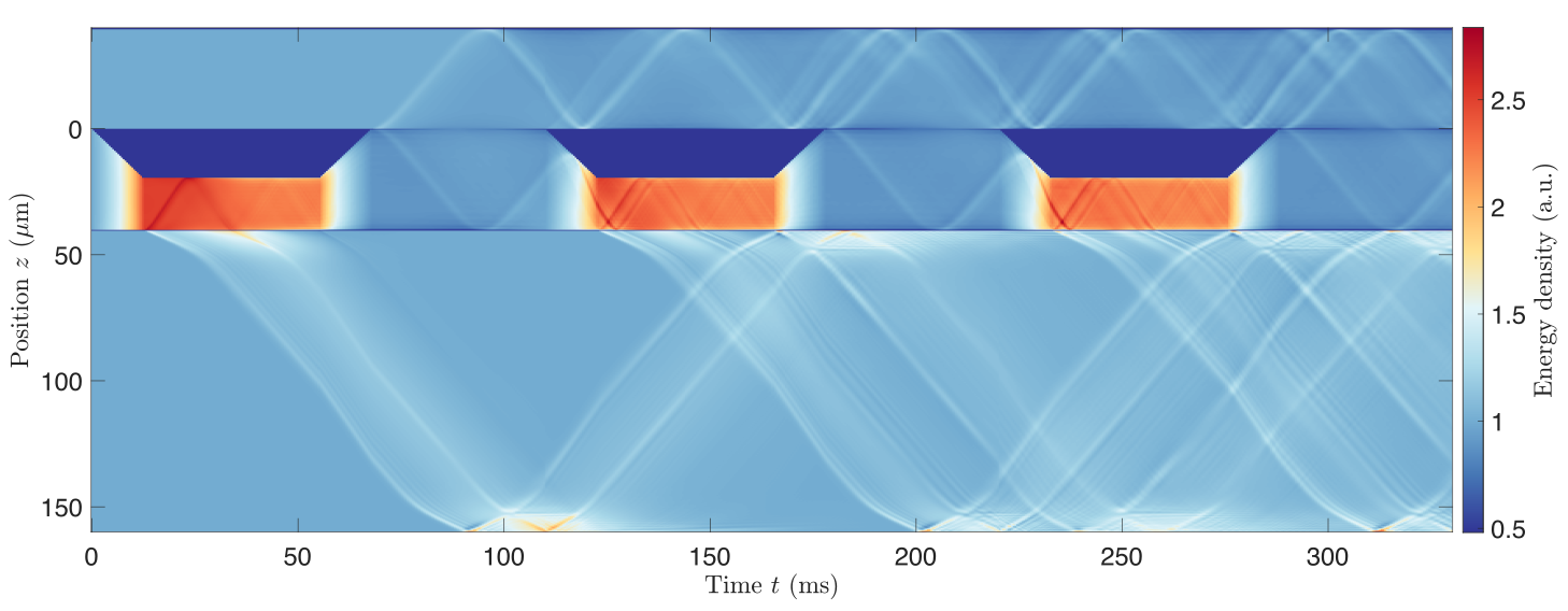
System
Piston
Bath
Bath with excitations
System cooled down
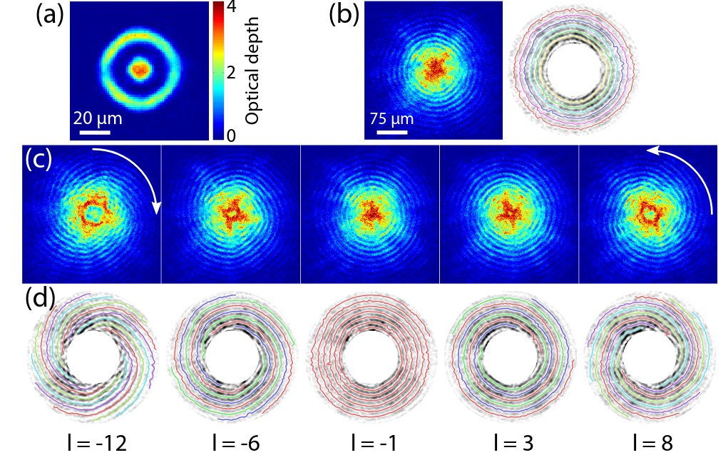
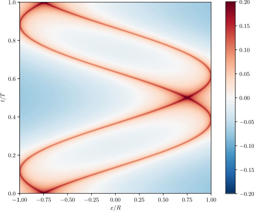
Breaking of the Huygens-Fresnel principle
in the inhomogenous TLL model:
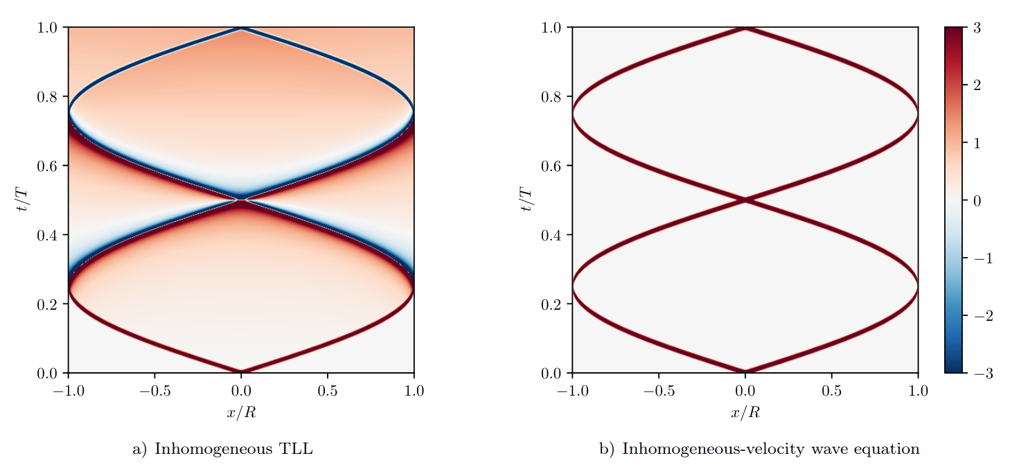
Why?
Why develop continuous field
quantum simulators?
- Representation theory: Quantum information?
- Continuum limits: BQP and QMA or more?
- Are nanowires computationally hard to simulate?
What do we know is difficult?


SM
Fundamental
Universal
Effective
Why develop continuous field
quantum simulators?
- Representation theory: Quantum information?
- Continuum limits: BQP and QMA or more?
- Are nanowires computationally hard to simulate?
What do we know is difficult?
SM
Fundamental
Universal
Effective
Non-thermal
steady states
Sine-Gordon
thermal states
Atomtronics
Generalized hydrodynamics
Recurrences
Some highlights:
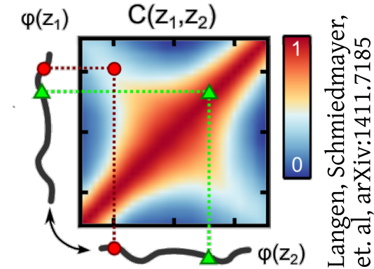
Interferometry measures velocities

van Nieuwkerk, Schmiedmayer, Essler, arXiv:1806.02626
Schumm, Schmiedmayer, Kruger, et al., arXiv:quant-ph/0507047
\partial_z\hat \varphi(z) \approx\frac{\hat \varphi(z)-\hat \varphi(z+\Delta z)}{\Delta z}
\partial_z\hat \varphi(z) \approx\frac{\Delta\hat\varphi(z)}{\Delta z}
\Delta z
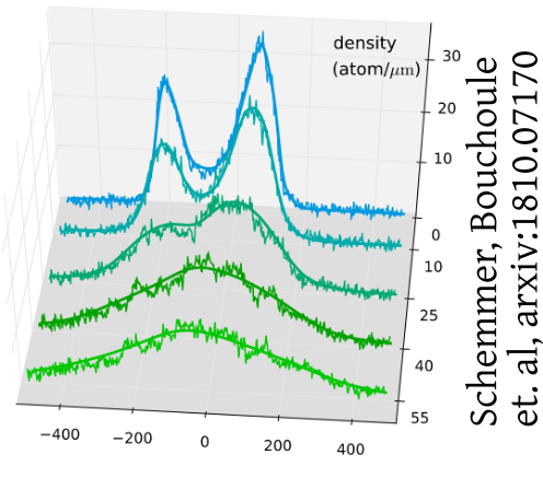
Tomography
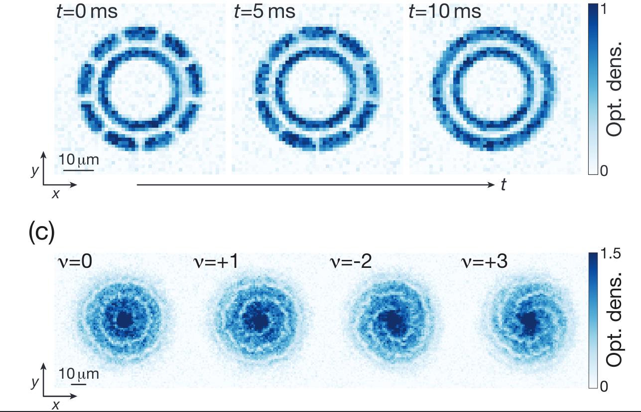
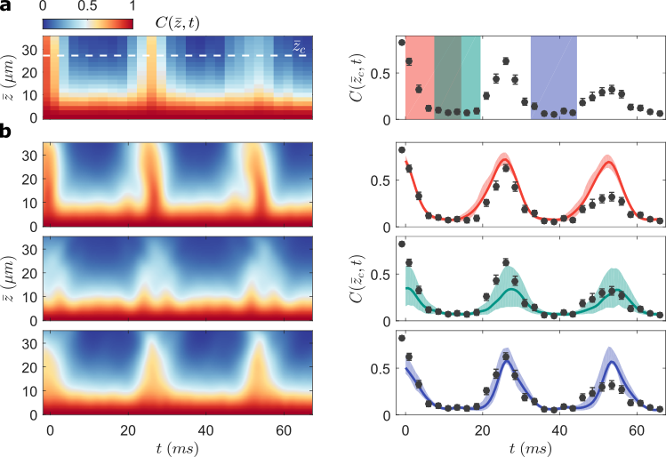
Tomography for phonons
\hat H_\text{TLL} = \int \text{d}z\left[ \frac{\hbar^2n_{GP}}{2m}\partial_z\hat\varphi^2+g\delta\hat\varrho^2\right]
\hat H_\text{TLL} = \sum_{k>0} \frac {\hbar \omega_k}2 (\phi_k^2+\delta\hat\rho_k^2) + g\hat\rho_0^2
\langle\hat \phi_k^2(t)\rangle= \cos^2(\omega_k t) \langle \phi_k^2(0)\rangle \\
\quad\quad\quad\quad\quad+\sin^2(\omega_k t) \langle \delta\hat \rho_k^2(0)\rangle

\delta \hat\rho
\langle\hat \phi^2(t)\rangle
\langle\delta\hat \rho^2(0)\rangle =0?
\langle \hat \phi^2(0)\rangle
\hat \phi
Tomography for phonons
\hat H_\text{TLL} = \int \text{d}z\left[ \frac{\hbar^2n_{GP}}{2m}\partial_z\hat\varphi^2+g\delta\hat\varrho^2\right]
\hat H_\text{TLL} = \sum_{k>0} \frac {\hbar \omega_k}2 (\phi_k^2+\delta\hat\rho_k^2) + g\hat\rho_0^2
\langle\hat \phi_k^2(t)\rangle= \cos^2(\omega_k t) \langle \phi_k^2(0)\rangle \\
\quad\quad\quad\quad\quad+\sin^2(\omega_k t) \langle \delta\hat \rho_k^2(0)\rangle
\delta \hat\rho
\langle\hat \phi^2(t)\rangle
\langle\delta\hat \rho^2(0)\rangle =0?
\langle \hat \phi^2(0)\rangle
\hat \phi
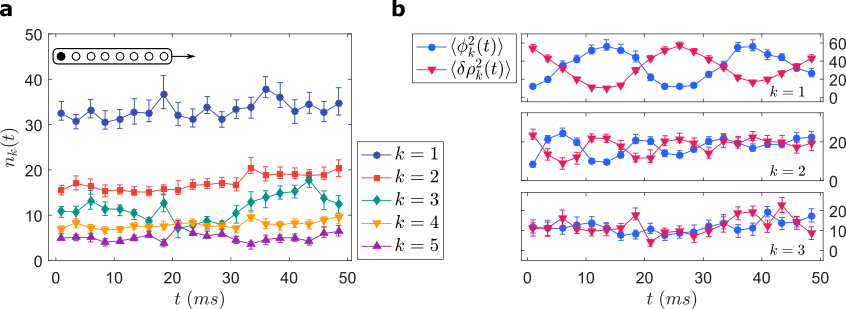
What are eigenmodes?
\hat H_\text{TLL} = \int \text{d}z\left[ \frac{\hbar^2n_{GP}}{2m}\partial_z\hat\varphi^2+g\delta\hat\varrho^2\right]
\hat H_\text{TLL} = \sum_{k>0} \frac {\hbar \omega_k}2 (\phi_k^2+\delta\hat\rho_k^2) + g\hat\rho_0^2
\hat \phi_k = \int_0^L dz \cos(\pi k z/L)\hat \varphi(z)
\int_0^L dz \cos(\pi k z/L)\cos(\pi k'z/L) = \delta_{k,k'}
Transmutation
\langle\hat \phi_k^2(t)\rangle= \cos^2(\omega_k t) \langle \hat\phi_k^2(0)\rangle +\sin^2(\omega_k t) \langle \delta\hat \rho_k^2(0)\rangle
\langle\hat \phi_k^2(t)\rangle= \langle \hat\phi_k^2(0)\rangle
\langle\hat \phi_k^2(t)\rangle= \langle \delta\hat \rho_k^2(0)\rangle
t=0:
t=\frac{\pi}{2\omega_k}:
\delta \hat\rho
\langle\hat \phi^2(t)\rangle
\langle\delta\hat \rho^2(0)\rangle =0?
\langle \hat \phi^2(0)\rangle
\hat \phi
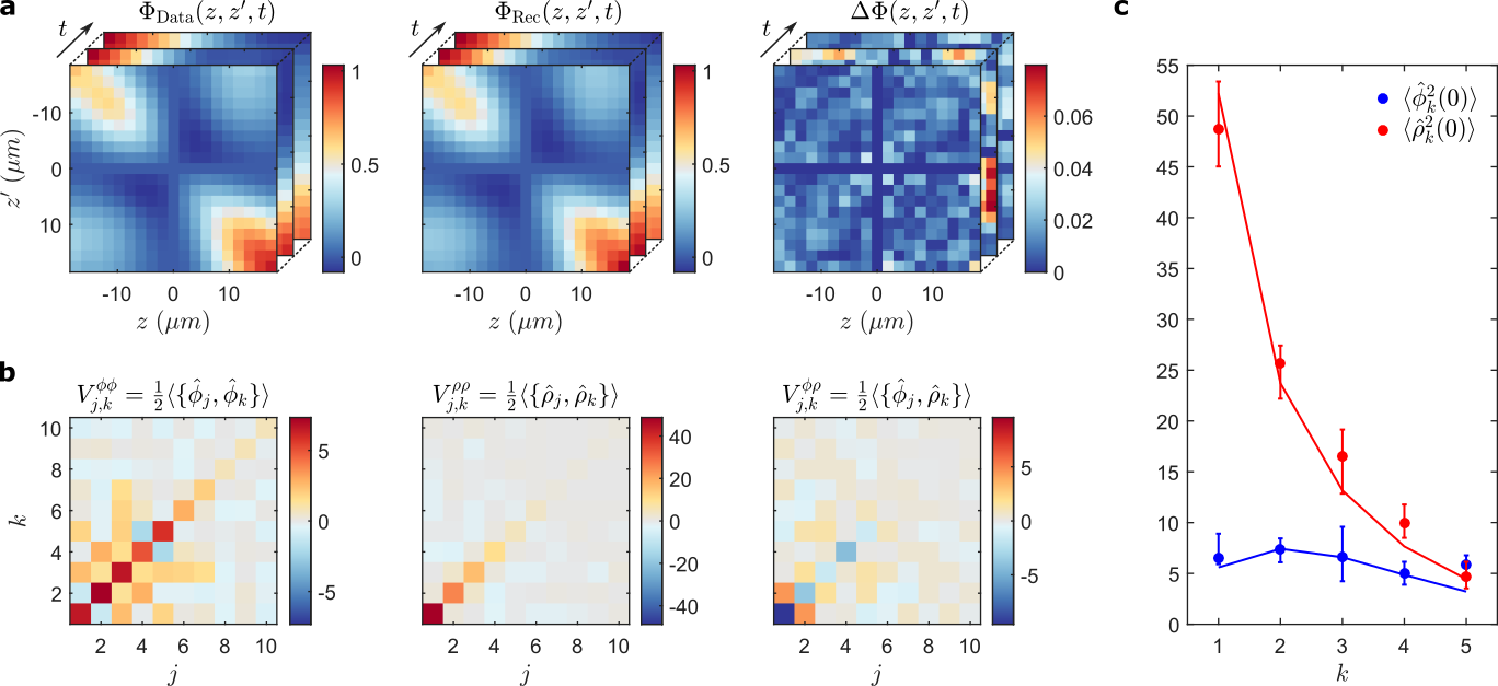
Tomography
A_{1,2}= \sin^2(\omega_k t_1 )
A_{1,1}= \cos^2(\omega_k t_1)
\langle\hat \phi_k^2(t)\rangle= \cos^2(\omega_k t) \langle \hat\phi_k^2(0)\rangle+ \sin^2(\omega_k t) \langle \delta\hat \rho_k^2(0)\rangle
A_{3,2}= \sin^2(\omega_k t_3 )
A_{3,1}= \cos^2(\omega_k t_3)
A_{2,2}= \sin^2(\omega_k t_2 )
A_{2,1}= \cos^2(\omega_k t_2)
A
\begin{pmatrix} \langle \hat\phi_k^2(0)\rangle \\\langle \delta\hat \rho_k^2(0)\rangle
\end{pmatrix}
=\begin{pmatrix} \langle \hat\phi_k^2(t_1)\rangle \\\langle \hat\phi_k^2(t_2)\rangle \\\langle \hat\phi_k^2(t_3)\rangle \end{pmatrix}
\|Aq - d\| = \text{min}
(This formalism: Tomography for many modes)

Tomography Klein-Gordon thermal state after quench
\hat H_\text{KG}=\hat H_\text{TLL}+J\int \mathrm{d}z \,n_{GP} \hat \varphi^2
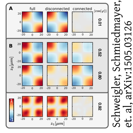
Extracting physical properties
Extracting physical properties
Extracting physical properties
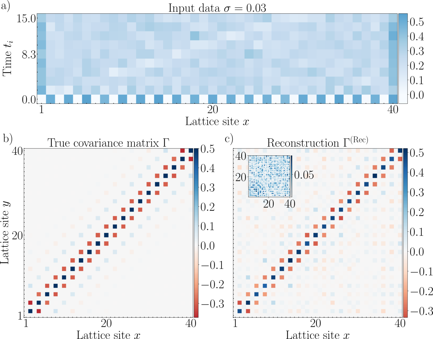
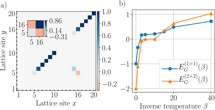
Tomography for optical lattices


Material science?
0
0
0
0
C
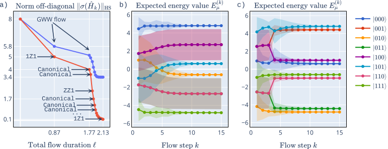
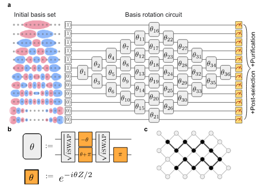
Diagonalization quantum algorithm
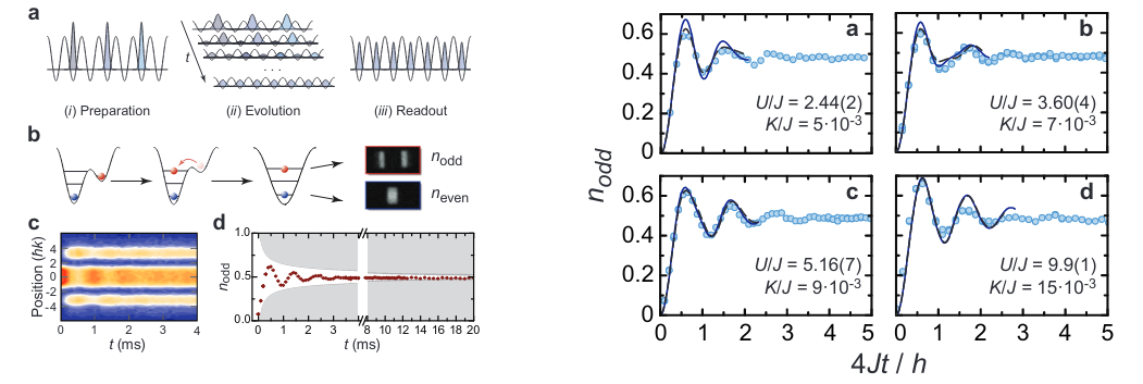
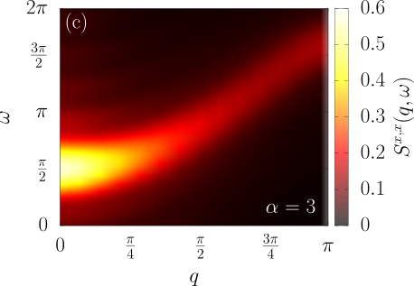
DSF of Rydberg arrays
Phonon tomography
Optical lattice tomography
\langle\hat \phi_k^2(t)\rangle= \cos^2(\omega_k t) \langle \phi_k^2(0)\rangle \\
\quad\quad\quad\quad\quad+\sin^2(\omega_k t) \langle \delta\hat \rho_k^2(0)\rangle
\delta \hat\rho
\langle\hat \phi^2(t)\rangle
\langle\delta\hat \rho^2(0)\rangle =0?
\langle \hat \phi^2(0)\rangle
\hat \phi
Ask me anytime:


0
0
0
0
C
Fidelity witnesses
Tomography optical lattices
Tomography phonons
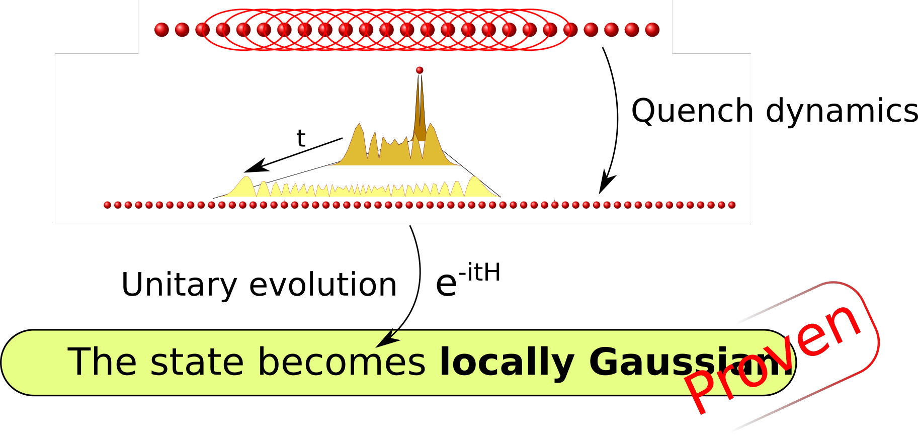
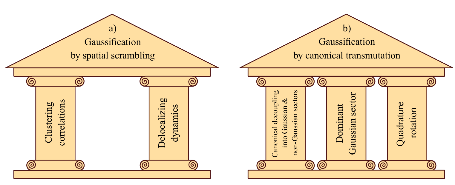
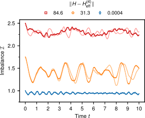
Proving statistical mechanics
Quantum simulating DSF
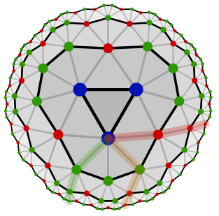
Holography in tensor networks
PEPS contraction average #P-hard
Quantum field machine
MBL l-bits
(click links at slides.com/marekgluza
Tutorial: Quantum simulation
By Marek Gluza


