EVOLVE
Particle Swarms for optimisation
Nicholas Browning
A Multi-objective Evolutionary Toolbox
Introduction
- Swarm Intelligence
- Applications
- Introduction to Particle Swarm Optimization (PSO)
- The Idea
- The Implementation (Vanilla)
- Topology
- PSO Variants
- Constriction PSO (CPSO)
- Fully informed PSO (FIPSO)
- Benchmark Functions
- Benchmark Analysis
- Cool Videos
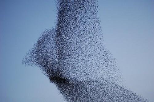
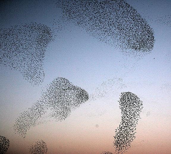
Swarm Intelligence
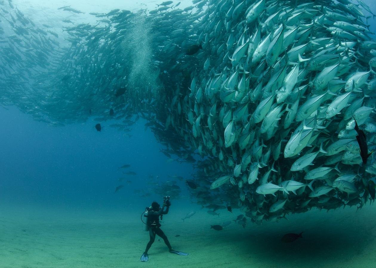
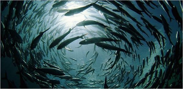
Swarm Intelligence
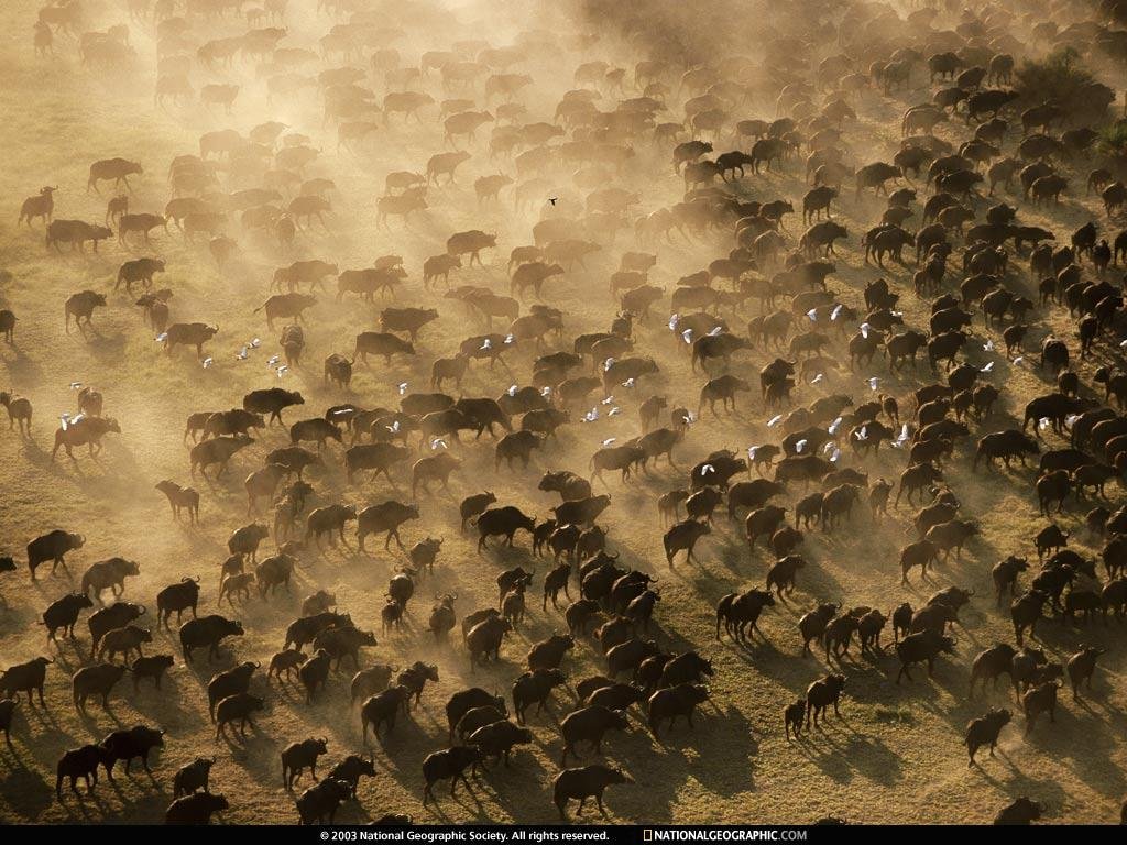
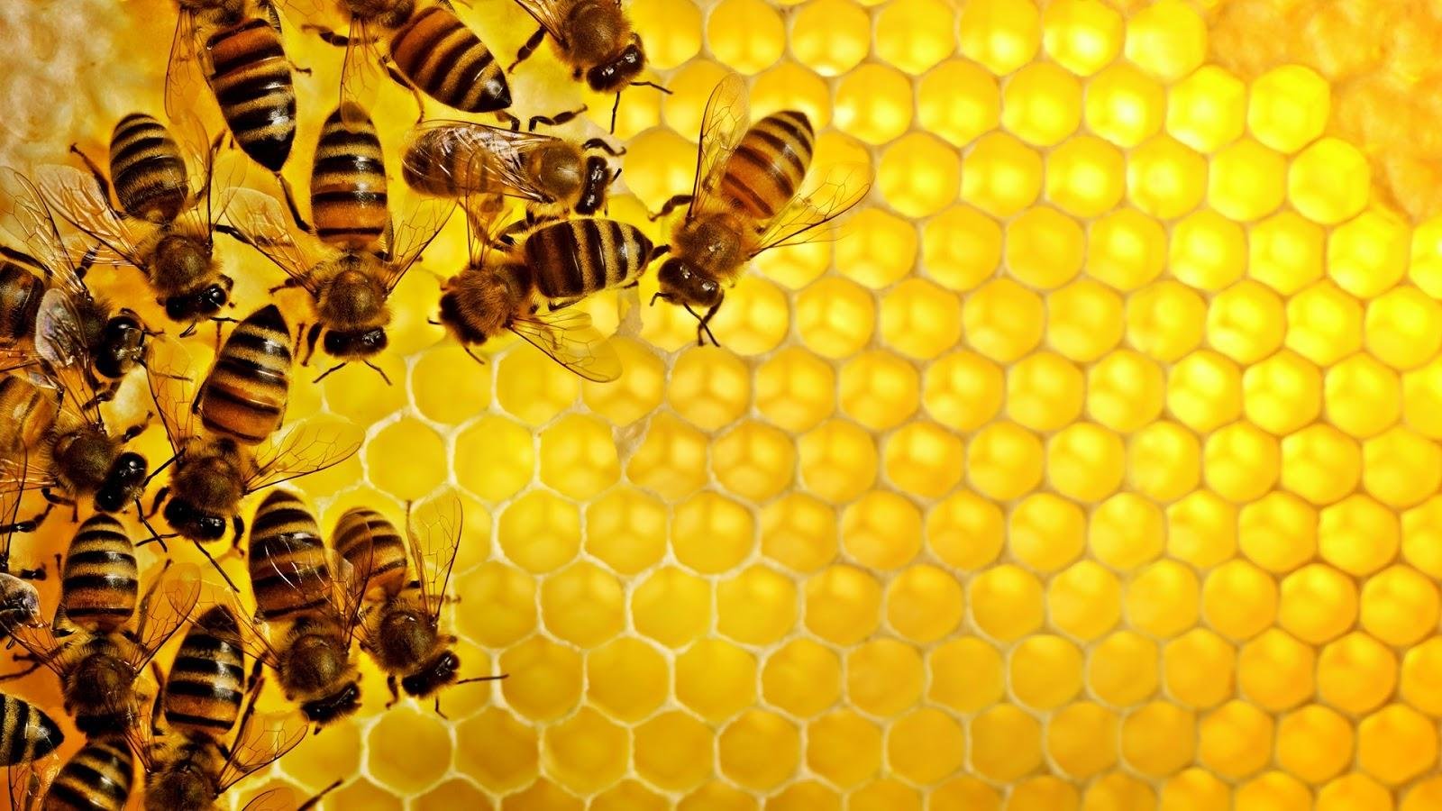
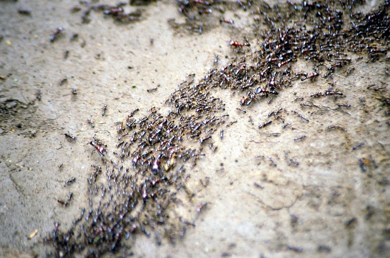
Swarm Intelligence
Artificial intelligence technique based on study of collective behaviour in decentralised, self-organised systems.
Population of simple "agents" capable of interacting locally, and with their enviroment.
Usually no centre of control - local interactions between agents usually leads to global behaviour
Swarm Intelligence
Swarm Intelligence

Sunderland A.F.C PSO?
Swarm Intelligence
5 tenets of swarm intelligence, proposed by Millonas [1]
- Proximity: simple space and time calculations
- Quality: respond to quality factors in the environment
- Diverse Response: activites must not occur along excessively narrow channels
- Stability: mode of behaviour should not change upon environment change.
- Adaptability: Mode of behaviour must be able to change if it's "worth" the computational price
[1] M. M. Milonas. Swarms, Phase Transitions, and Collective Intelligence. Artificial Life III, Addison Wesley, Reading, MA, 1994.
Applications

Also Batman, LOTR, Lion king, Happy Feet...
Particle Swarm Optimisation
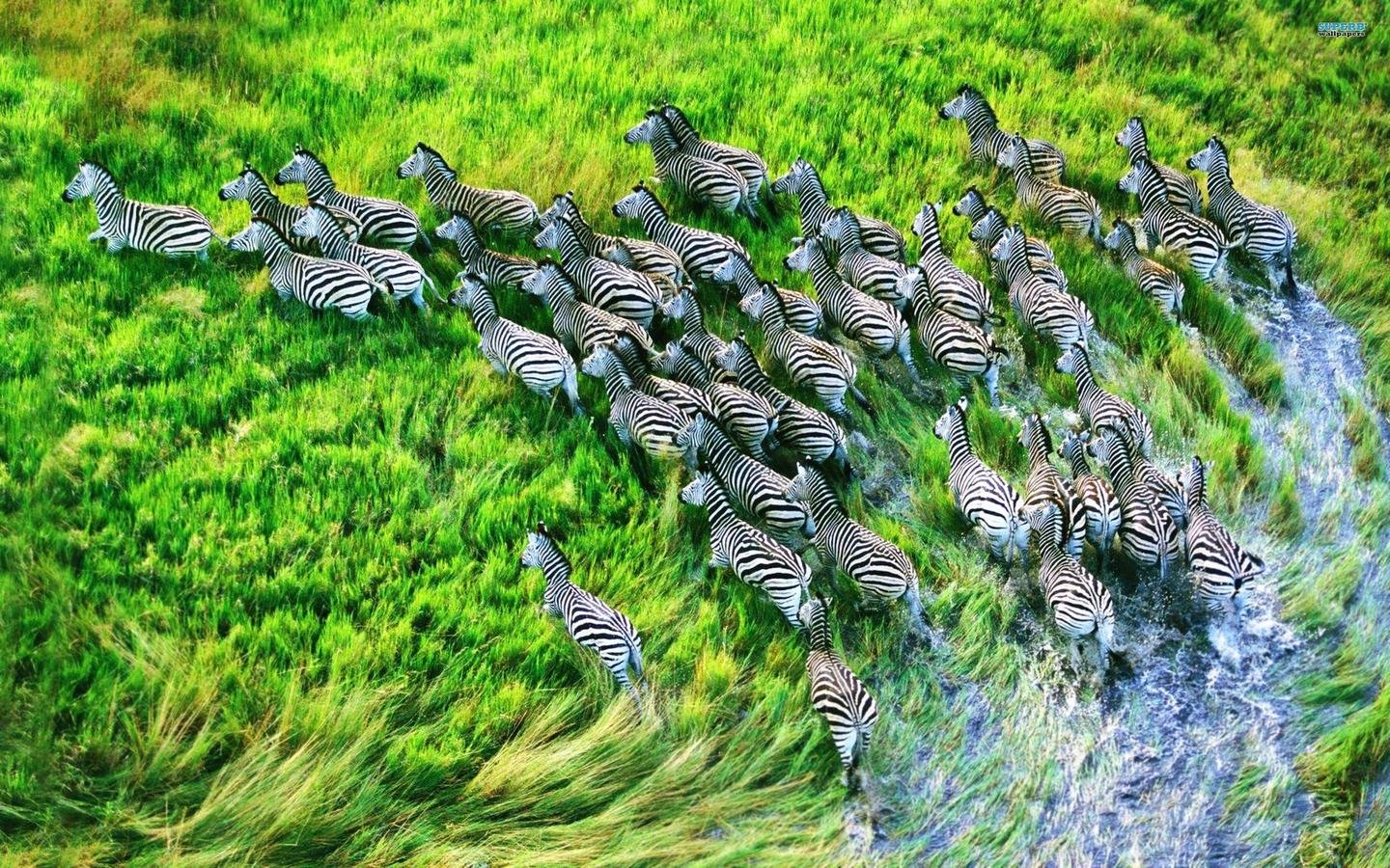
First proposed by J. Kennedy and R. Eberhart [2], intent to imitate social behaviour of animals which display herding/swarming characteristics.
Each individual in the swarm learns from both its own past experiences (cognitive behaviour) and also from its surrounding neighbours (social behaviour).
Optimisation was not intentional!
[2] Kennedy, J.; Eberhart R., Particle Swarm Optimisation, Proc. Int. Conf. Neural Networks, 1995.
\vec{X}_i = \vec{X}_{min} + \vec{U}[0, 1] \odot (\vec{X}_{max} - \vec{X}_{min})
X⃗i=X⃗min+U⃗[0,1]⊙(X⃗max−X⃗min)
\vec{V}_i^t = (-\vec{X}_{min} + \vec{U}[0, 2] \odot (\vec{X}_{max} - \vec{X}_{min}))
V⃗it=(−X⃗min+U⃗[0,2]⊙(X⃗max−X⃗min))
Each particle is initialized in space:
Each particle must move and hence has a velocity:
The Implementation (Vanilla)
The Implementation (Vanilla)
How is cognitive and social learning achieved?
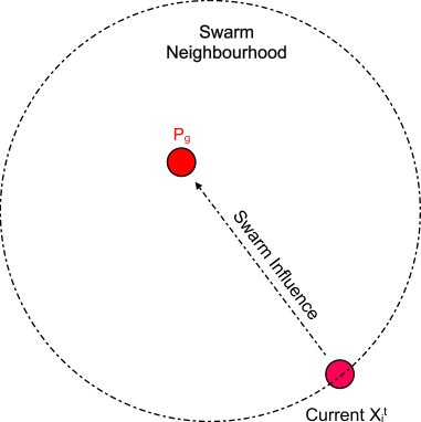
COGNITIVE AND SOCIAL INFLUENCE
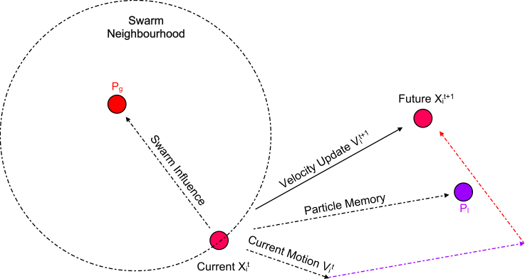
\vec{V}_i^{t+1} = w\vec{V}_i^t + \vec{U}[0, c_l]\odot(\vec{P}_i - \vec{X}_i^t) + \vec{U}[0, c_g] \odot (\vec{P}_g - \vec{X}_i^t)
\vec{X}_i^{t+1} = \vec{X}_i^t + \vec{V}_i^{t+1}\Delta t
The Implementation (Vanilla)
Velocity update is defined by:
New particle position can then be calculated:
Cognitive Influence
Swarm Influence
\vec{P}_m = \frac{(\vec{U}[0, c_l] \odot P_i +\vec{U}[0, c_g] \odot P_g)} {\vec{U}[0, c_l] + \vec{U}[0, c_g] }
Particle will cycle unevenly about the point:
SWARM NEIGHBOURHOOD: TOPOLOGY
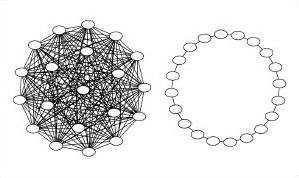
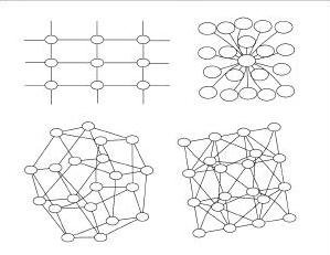
All
Ring
2D Von Neumann
3D Von Neumann
Star
Pyramid
Many graph representations possible!
Clerc [3] adapted PSO algorithm to include constriction coefficient. Convergence guaranteed, but not necessarily to global optimum.
Eberhart and Shi [4] later proposed modified version with improved performance
\vec{V}_i^{t+1} = K[\vec{V}_i^t + \vec{U}[0, c_l]\odot (\vec{P}_i^l - \vec{X}_i^t) + \vec{U}[0,c_g]\odot(\vec{P}_g - \vec{X}_i^t)]
Constriction PSO
[3] M. Clerc. The Swarm and the Queen: Towards a Deterministic and Adaptive Particle Swarm Optimisation, Evolutionary Computation, 1999.
[4] R. C. Eberhart, Y. Shi. Comparing Inertia Weights and Constriction Factors in Particle Swarm Optimisation, Evolutionary Computation, 2000.
K = \frac {2} {|2 - \psi - \sqrt{\psi^2 -4\psi}}
\psi = c_l + c_g; \psi > 4
Particle searches through it's neighbours to identify the one with the best result: biases the search in a promising direction
Fully informed PSO
Perhaps chosen neighbour is in fact not in a better region, and is simply heading toward a local optima?
Important information may be neglected through overemphasis on a single best neighbour
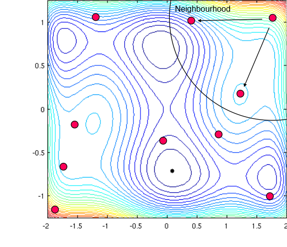
Fully informed PSO
\vec{V_i^{t+1}} = K[\vec{V}_i^t + \frac{1}{N_i}\sum_{j=1}^{N_i}U(0, \psi) \odot (\vec{P}_j - \vec{X}_i^t)]
\psi > 4
K = \frac {2} {|2 - \psi - \sqrt{\psi^2 -4\psi}}
Mendes et al. [5] proposed a PSO variant which captures a weighted average influence of all particles in neighbourhood. Poli et al. [6] proposed the following simplified FIPSO update equation:
[5] R. Mendes, J. Kennedy, and J. Neves. The Fully Informed Particle Swarm: Simpler, Maybe Better. IEEE Transactions on Evolutionary Computation, 2004.
[6] R. Poli, J. Kennedy and T. Blackwell. Particle Swarm Optimisation: An Overview. Swarm Intell., 2007.
Benchmark functions
De Jong's Standard Sphere Function
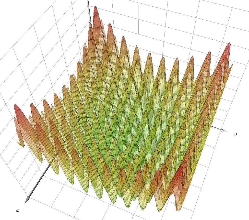
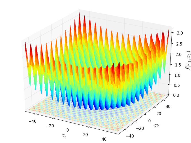
Eggcrate Function
h(\vec x) = \sum_{i=1}^{d} x_i^2
g(x, y) = x^2 + y^2 + 25(\sin^2(x) + \sin^2(y))
h_{min} (\vec x) = 0; \vec x = 0
g_{min} (x, y) = 0; x,y = 0
Benchmark functions
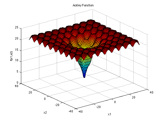
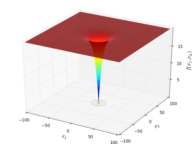
Ackley's Function
s(\vec{x}) = 20 + e -20\exp{[-0.2 \sqrt{\frac{1}{d} \sum_{i=1}^{d} x_i^2}] - \exp{[\frac{1}{d}\sum_{i=1}^d cos(2 \pi x_i)}]}
s_{min} (\vec x) = 0; \vec x = 0
-30 \leq x_i \leq 30
Benchmark functions
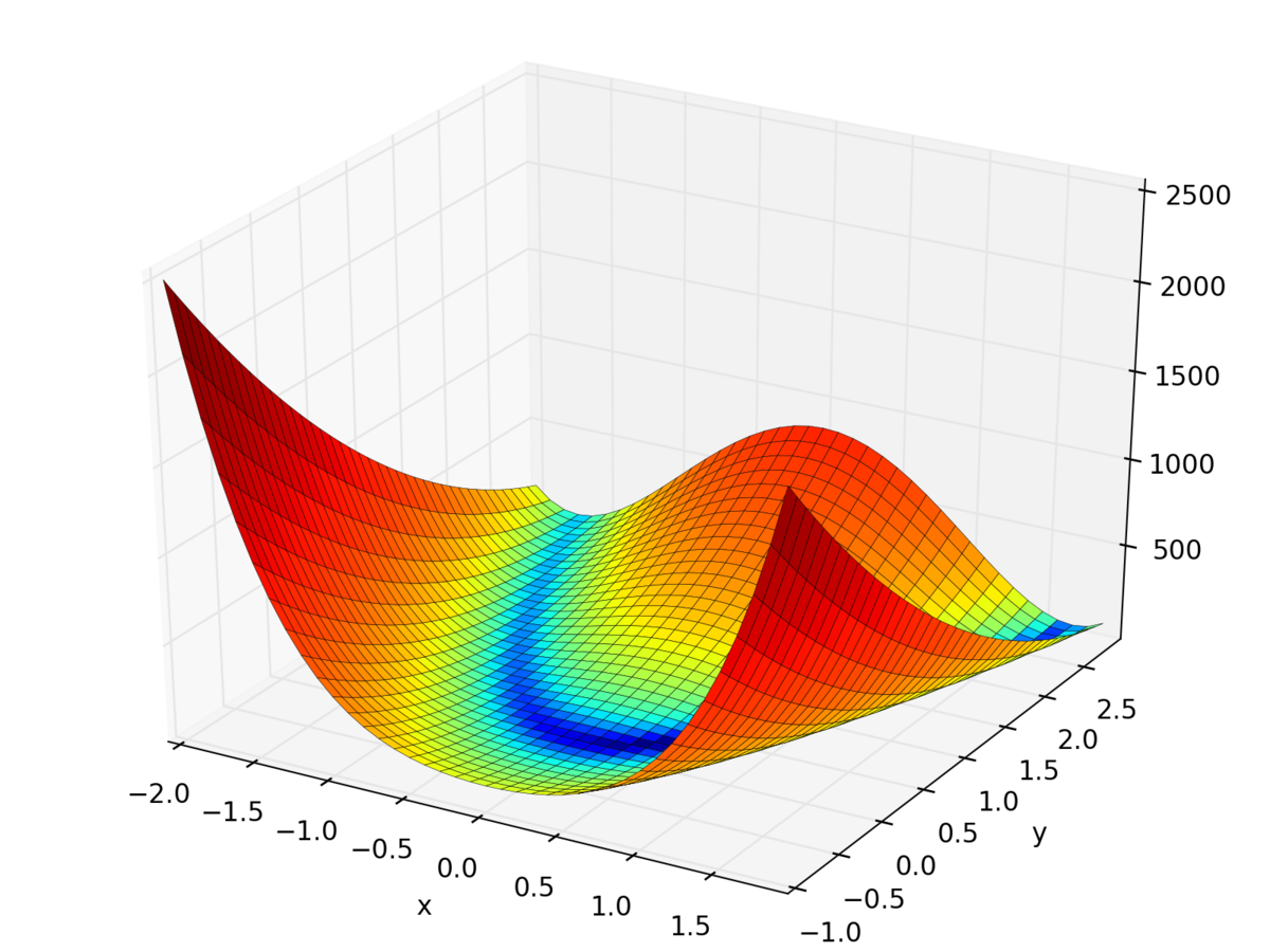
Rosenbrock's Function
Michaelewicz's Function
f(\vec{x}) = - \sum _{i=1}^d sin(x_i)[sin(\frac{ix_i^2}{\pi})]^{2m}
f(\vec{x}) = \sum_{i=1}^{d-1} [(1-x_i)^2 + 100(x_{i+1} - x_i^2)^2]
-2048 \leq x_i \leq 2048
f_{min} (\vec x) = 0; \vec x = 0
d! local minima in domain
0 \leq x_i \leq \pi
where i = 1, 2, ..., d
f_{min} ^ {d=2} \approx -1.801
f_{min} ^ {d=5} \approx -4.6877
Benchmark functions
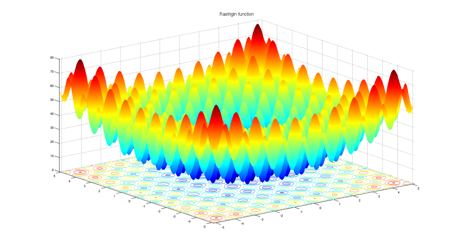
Rastrigrin's Function
Griewank's Function
f (\vec{x}) = 1 + \frac{1}{4000} \sum_{i=1}^d x_i^2 - \prod_{i=1}^d\cos{\frac{x_i}{\sqrt{i}}}
-600 \leq x_i \leq 600
f_{min} (\vec{x}) = 0; \vec x = 0
f(\vec x) = Ad + \sum_{i=1}^d(x_i^2 - A\cos{2\pi x_i})
A = 10; x \in [-5.12, 5.12]
f_{min}(\vec x) = 0 ; \vec x = 0
Benchmark functions
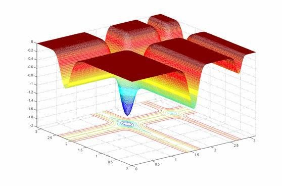
f(x, y) = -\cos{x}\cos{y}\exp{(-(x-\pi)^2-(y-\pi)^2})
Easom's Function
f_{min}(x, y) = -1; (\pi, \pi)
x,y \in [-100, 100]
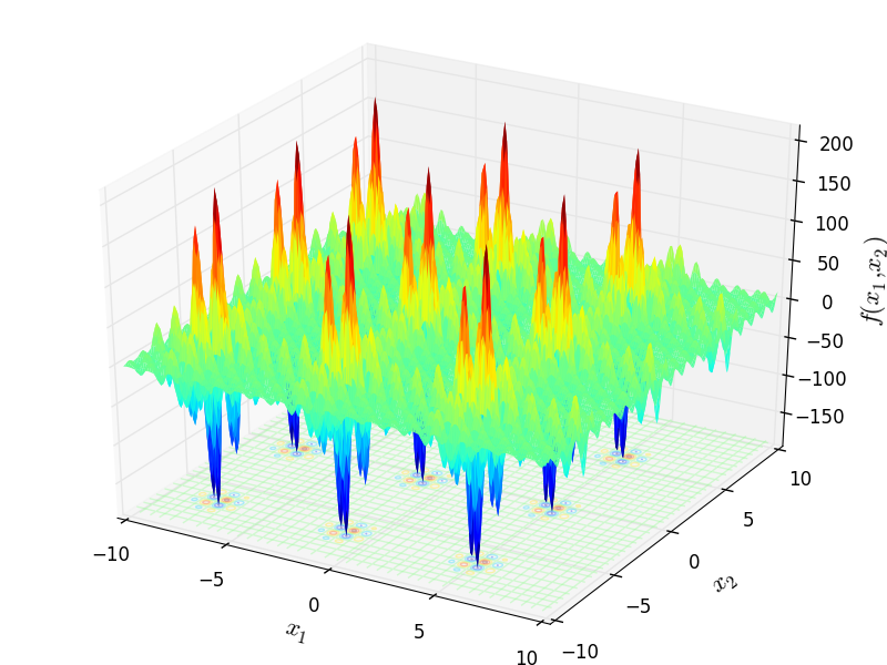
f(x, y) = (\sum_{i=1}^5i\cos{(i+1)x + i})(\sum_{i=1}^5i\cos{(i+1)y + i})
Shubert's Function
f_{min}(x, y) = -186.7309
x,y \in [-10, 10]
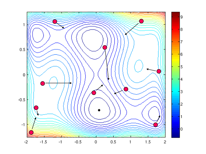
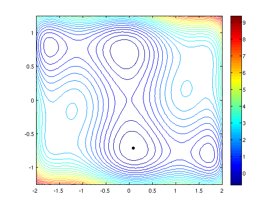
Dynamics Visualisation
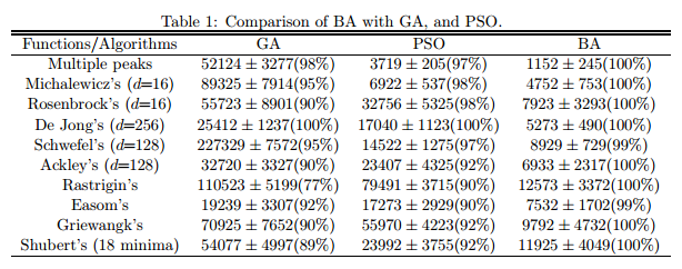
Benchmark Analysis
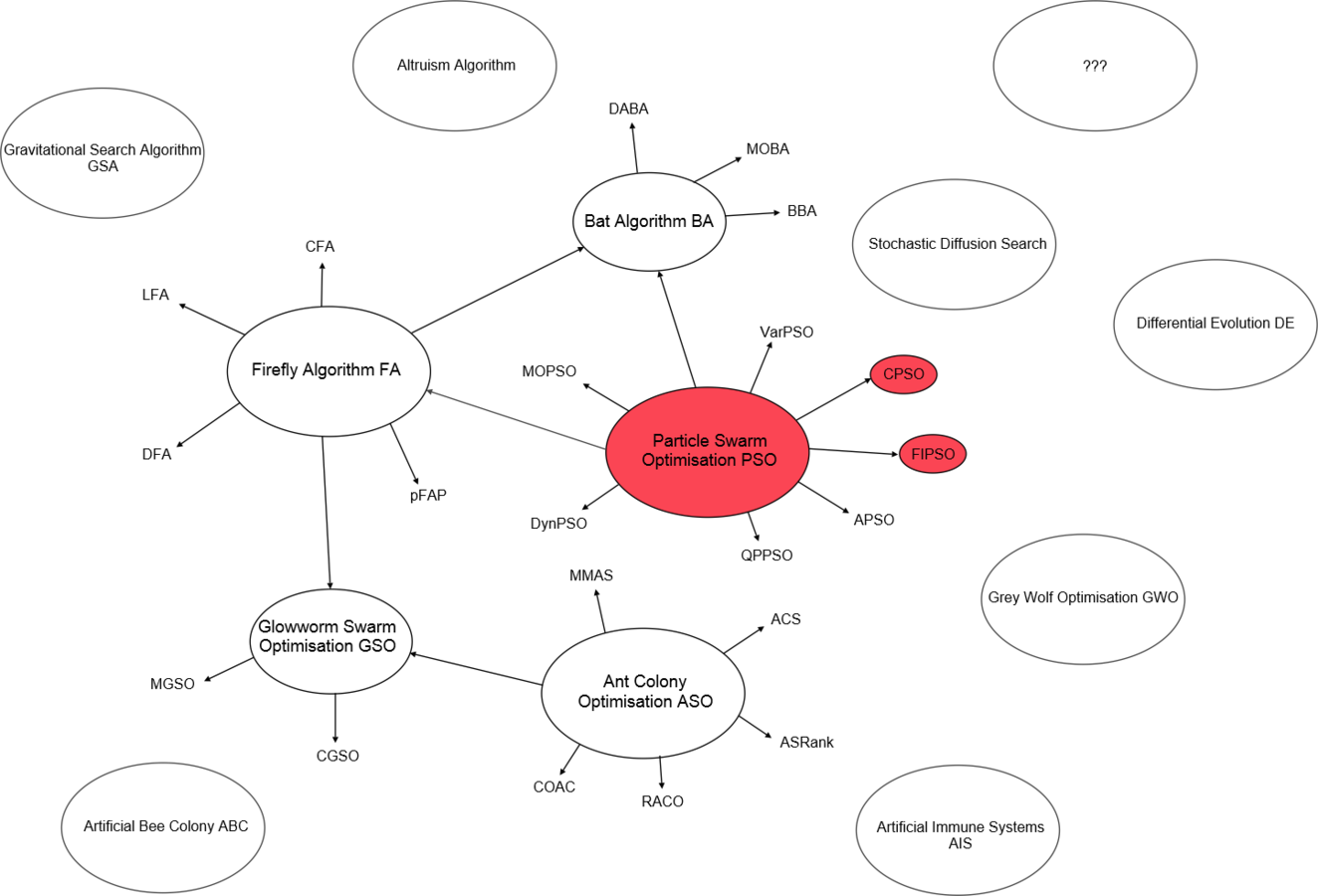
Comparison performed by Yang [7] - study introduces new PSO variant: "The Bat Algorithm"
[7] X. S. Yang. A New Metaheurstic Bat-Inspired Algorithm. Nature Inspired Cooperative Strategies for Optimisation, 2010.
Dynamic Optima
PSO in Theatre
Glowworm swarm Optimisation
Bat swarm algorithm
Special variant of PSO
Other similar ideas exist e.g Glowworm algorithm
based on the echolocation behaviour of microbats with varying pulse rates of emission and loudness.
TODO
EVOLVE - Particle Swarms for Optimisation
By Nick Browning


