Contact Detection from Joint Torque Measurements
\newcommand{\rv}[1]{\mathsfit{#1}}
\newcommand{\rvv}[1]{\bm{\mathsfit{#1}}}
Pang, joint work with Jack
Motivation
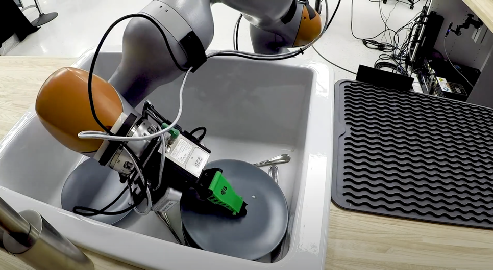
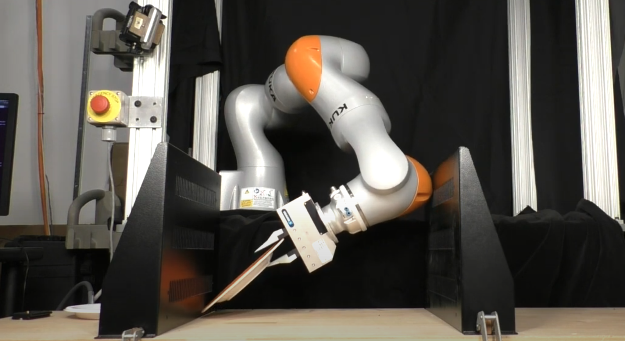
- Robots can and do make contact with the environment when they are working, e.g. picking up plates.
- We want the robot to keep working despite contacts.
- To accomplish that goal, an important component is knowing where the contact is.
- Tactile skins are nice, but can be fragile and cumbersome.
- Joint torque sensors are readily available and more robust.
Three ways to detect contact from joint torques
- Method by Haddadin
- Sampling-based methods, e.g. Contact Particle Filter.
- "Gradient descent" (our work)
Method by Haddadin
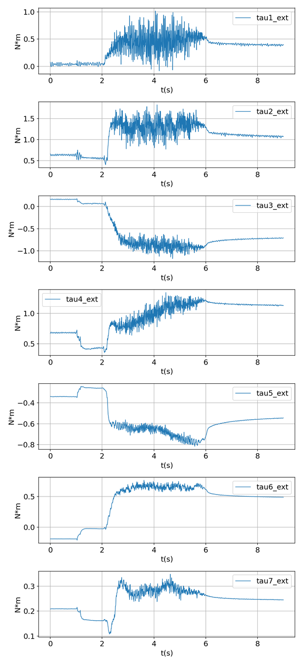
- Identify the link in contact as the last link with non-zero torque measurement.
$$\bm{\tau}_\text{ext} = \left[ \tau_1, \tau_2, \dots, \tau_{\textcolor{blue}{i_c}}, 0, 0, 0\right]$$
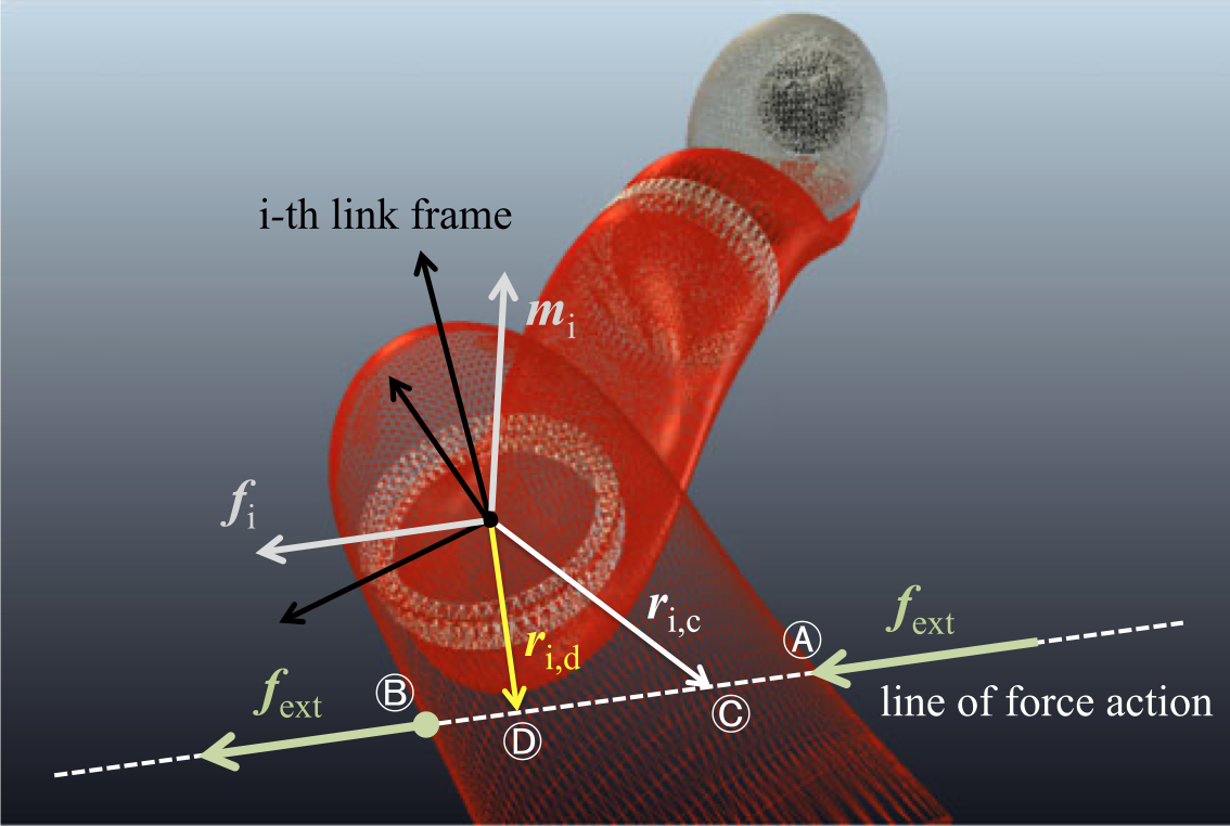
- Solve for \( \bm{m}_{i_c}, \bm{f}_{i_c} \) from
- Assume that \( \bm{m}_\text{ext} = 0 \), and solve for the line of action of \( \bm{f}_\text{ext} \) from
- Intersect the line with \(\mathcal{S}_{i_c}\), the surface of link \(i_c\).
Haddadin, Sami, Alessandro De Luca, and Alin Albu-Schäffer. "Robot collisions: A survey on detection, isolation, and identification." IEEE Transactions on Robotics 33.6 (2017): 1292-1312.
\bm{J}_{L_{i_c}}^\intercal
\begin{bmatrix}
\bm{m}_{i_c} \\
\bm{f}_{i_c}
\end{bmatrix}
= \bm{\tau}_\text{ext}
\begin{bmatrix}
\bm{I}_3 & \textcolor{blue}{\hat{\bm{p}}} \\
\bm{0}_3 & \bm{I}_3
\end{bmatrix}
\begin{bmatrix}
\bm{0} \\
\bm{f}_\text{ext}
\end{bmatrix}
=
\begin{bmatrix}
\bm{m}_{i_c} \\
\bm{f}_{i_c}
\end{bmatrix}
geometric Jacobian of frame \(L_{i_c}\)
Pitfalls
- \(\bm{\tau}_\text{ext}\) is almost always not zero.
- Biased due to imperfect calibration of EE inertia.
- Noisy due to robot motion.
- Instead of \(|\tau_i| = 0 \), Haddadin proposed checking \(|\tau_i| \leq \epsilon \).
- The contact detector makes a mistake when \(\bm{f}\) is on link \(i_c\) but \(|\tau_{i_c}| \leq \epsilon \).
$$\bm{q}_1$$
$$\bm{q}_2$$
Moving...
Thresholding joint torque
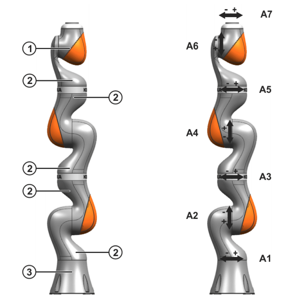
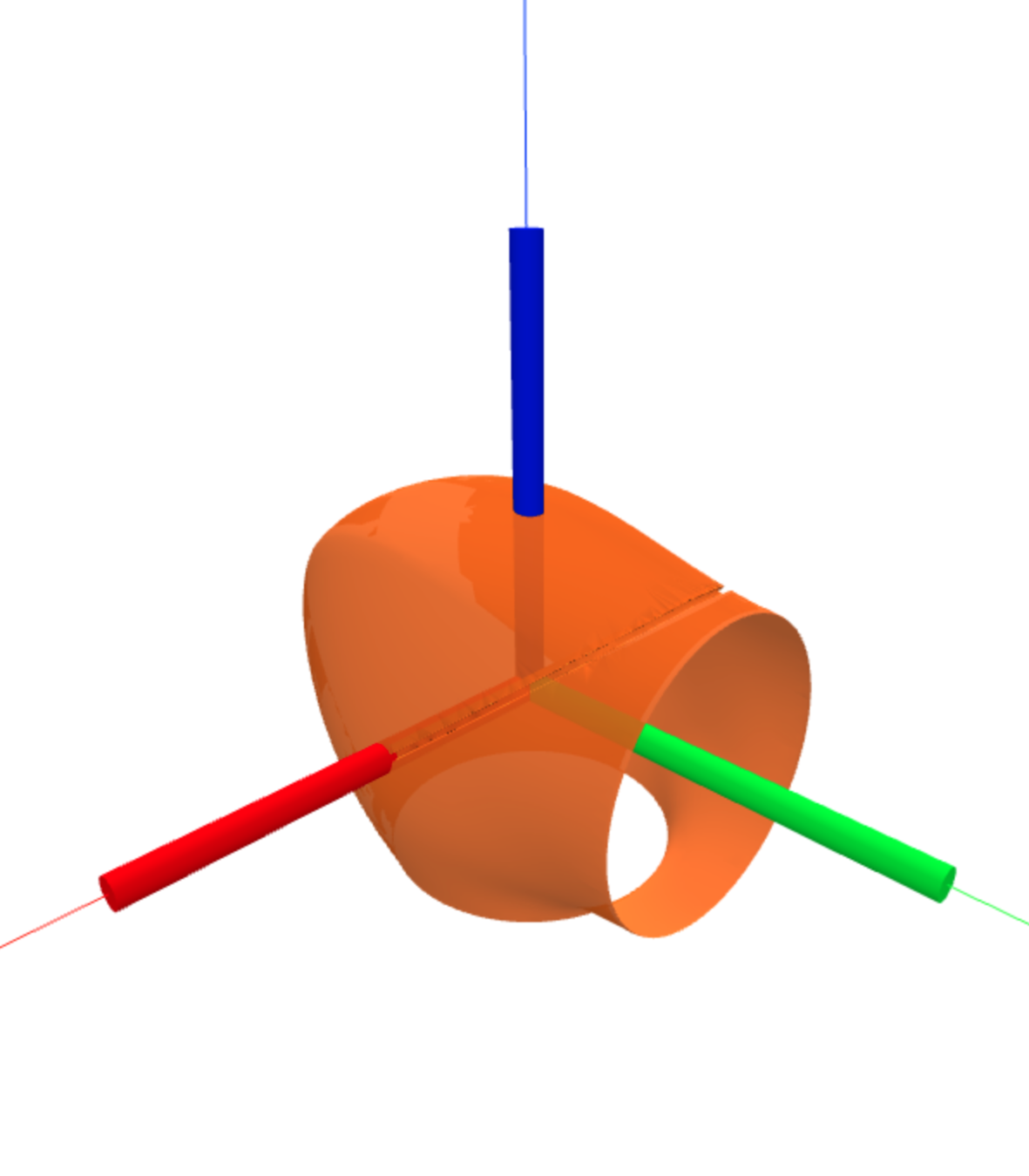
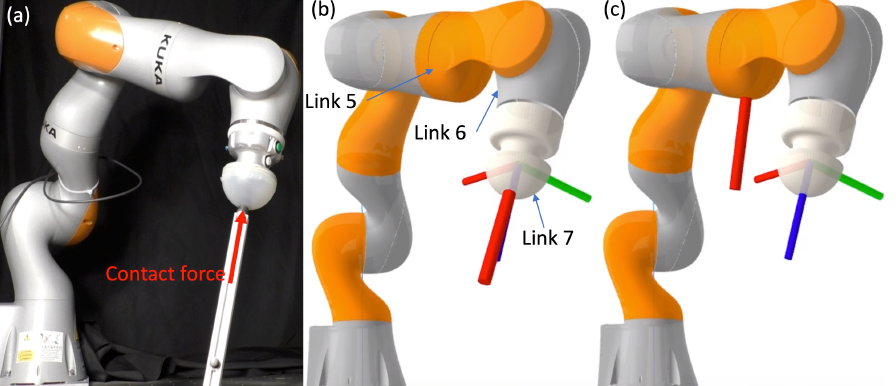
- Using link 6 of the IIWA robot as an example.
- Only the \(z\) component of \(\bm{m} = \bm{p} \times \bm{f}\) is sensed by the joint torque sensor.
- Thresholding \( |\tau_6| = |m_z| = |-p_y f_x + p_x f_y|\leq \epsilon \) : a linear constraint on the projection of \(\bm{f}\) onto the \(xy\) plane.
Link 6 of IIWA in its local coordinate frame.
\bm{p}
\bm{f}
\bm{p}_{xy}
\bm{f}_{xy}
p_y
p_x
f_x
f_y
\frac{2 \epsilon }{p_x}
x
y
z
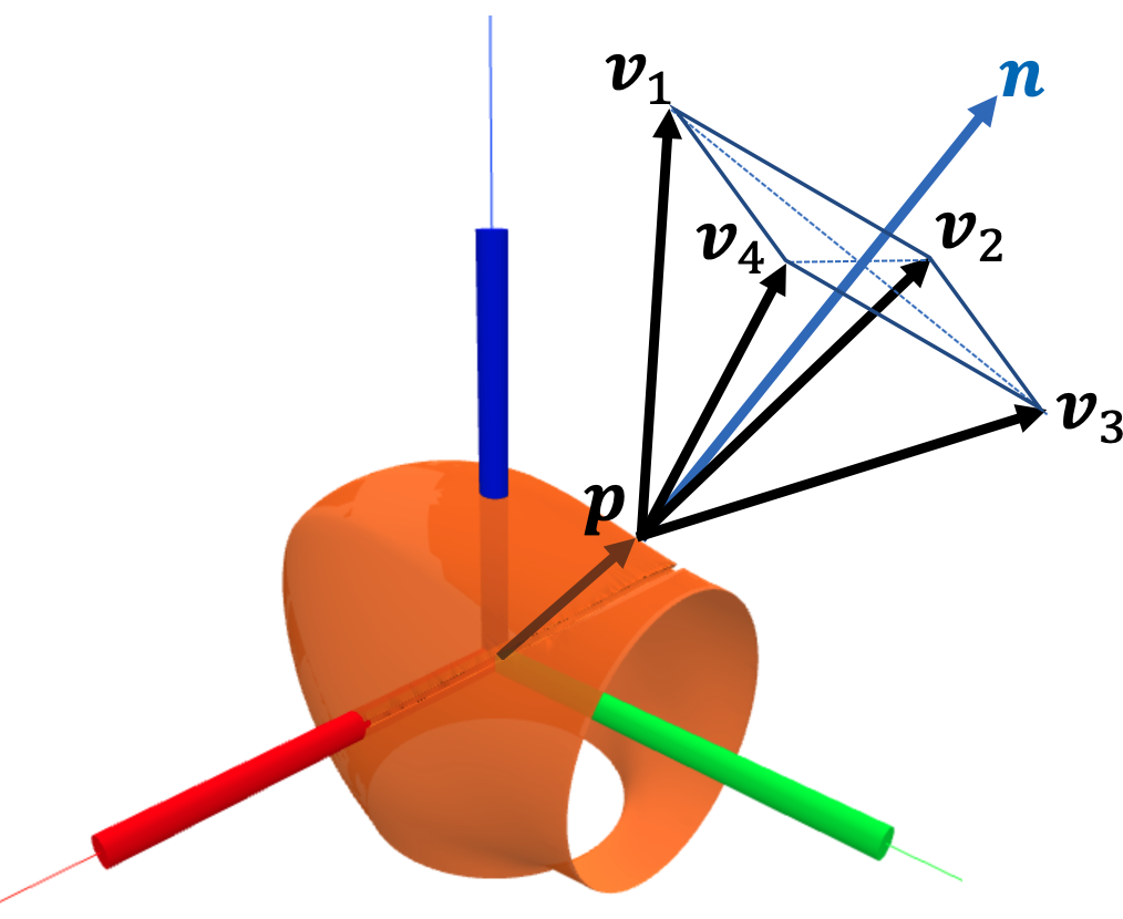
Computing the probability of \(|\tau_i| \leq \epsilon\)
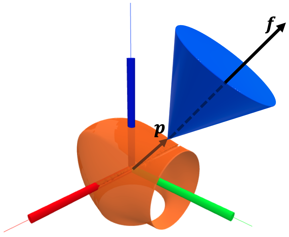
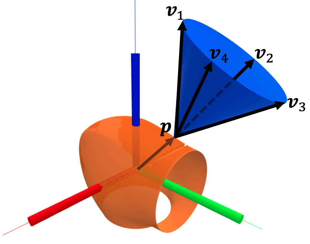
For a sampled point \( \bm{p} \) on the surface of the link:
- Sample forces of magnitude \(1\text{N}\) inside the friction cone at \( \bm{p} \).
- Project force samples onto the \(xy\) plane.
- Count number of samples inside the "band of small torque".
- Error probability = (# small torque samples) / (# all samples)
- Force samples on friction cone.
- Projected samples.
- Small-torque samples.
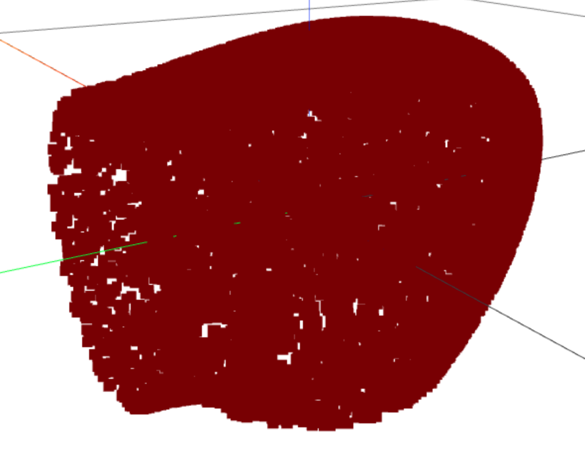
Space of contact force \(\bm{f}\)
Results
Space of contact force \(\bm{f}\)
$$\mu=1, \; \epsilon / \|\bm{f}\| = 0.01 \; \left(\text{N} \cdot \text{m} / \text{N}\right)$$

Probability: 0
1
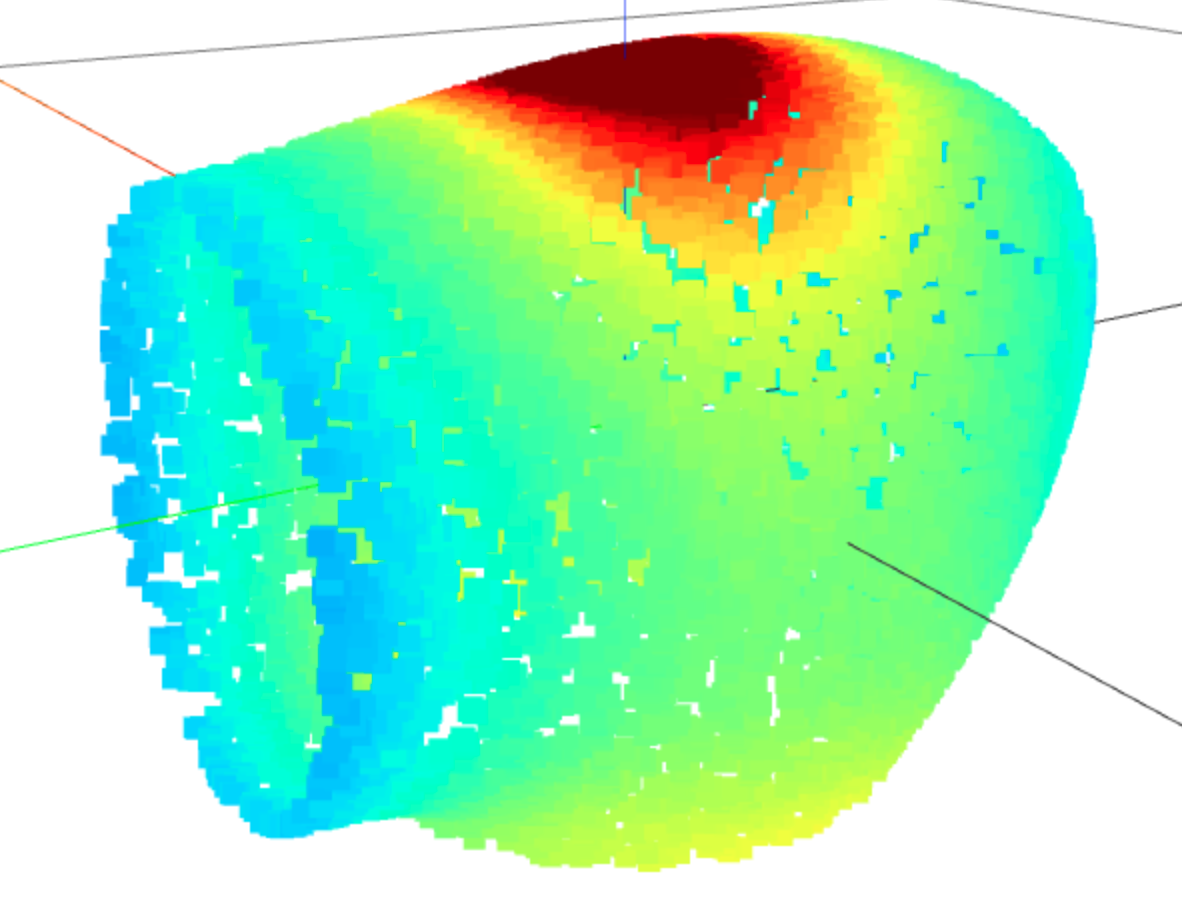
\mu=1, \; \epsilon / \|\bm{f}\| = 0.1 \; \left(\text{N} \cdot \text{m} / \text{N}\right)
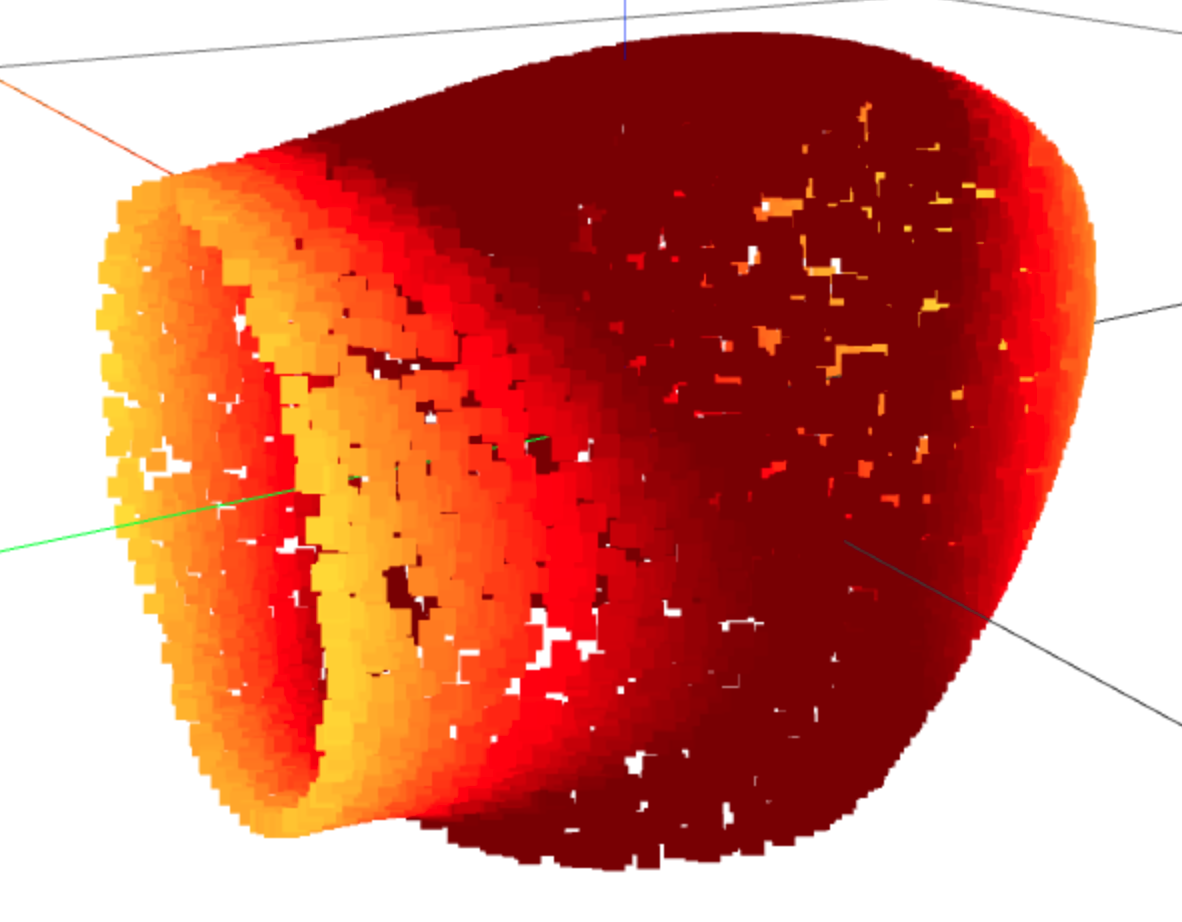
\mu=1, \; \epsilon / \|\bm{f}\| = 0.05 \; \left(\text{N} \cdot \text{m} / \text{N}\right)
\mu=1, \; \epsilon / \|\bm{f}\| = 0.02 \; \left(\text{N} \cdot \text{m} / \text{N}\right)
Thresholding joint torque
- Instead of \(|\tau_i| = 0 \), Haddadin proposed checking \(|\tau_i| \leq \epsilon \).
- Only the \(z\) component of \(\bm{m} = \bm{p} \times \bm{f}\) is sensed by the joint torque sensor.
- Thresholding \( |\tau_6| = |m_z| = |-p_y f_x + p_x f_y|\leq \epsilon \) : a linear constraint on the projection of \(\bm{f}\) onto the \(xy\) plane.
Link 6 of IIWA in its local coordinate frame.
x
y
z
\bm{p}
\bm{f}
\bm{p}
\bm{f}
p_y
p_x
f_x
f_y
\frac{2 \epsilon }{p_x}
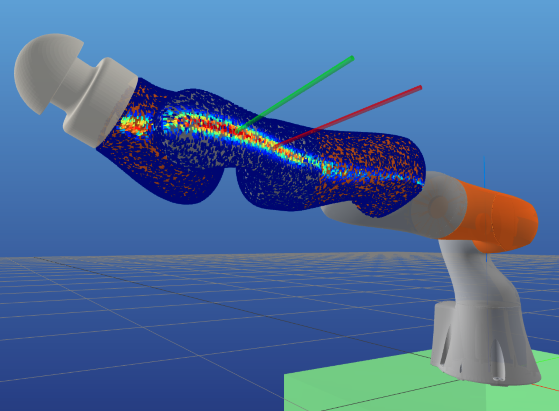
Contact Particle Filter
- For a given joint configuration \( \bm{q} \) and a joint torque measurement \(\bm{\tau}_\text{ext} \), if \(\bm{\tau}_\text{ext} \) is generated by a single external contact, there exists \( \bm{p} \in \mathcal{S} \) (robot surface) s.t. \( \| \bm{J}(\bm{q}, \bm{p})^{\intercal} \bm{v_f} - \bm{\tau}_\text{ext} \|^2 = 0, \bm{v_f} \geq 0\).
- To find \(\bm{p}\), we would like to solve
- But the constraint that \( \bm{p} \) stays on the surface of the robot, \( \bm{p} \in \mathcal{S} \), is difficult to deal with.
- Instead, samples are drawn from \( \mathcal{S} \) so that \( \bm{p} \) is fixed for each sample.
- By replacing the friction cone with a polyhedral cone, the optimization above becomes a QP:
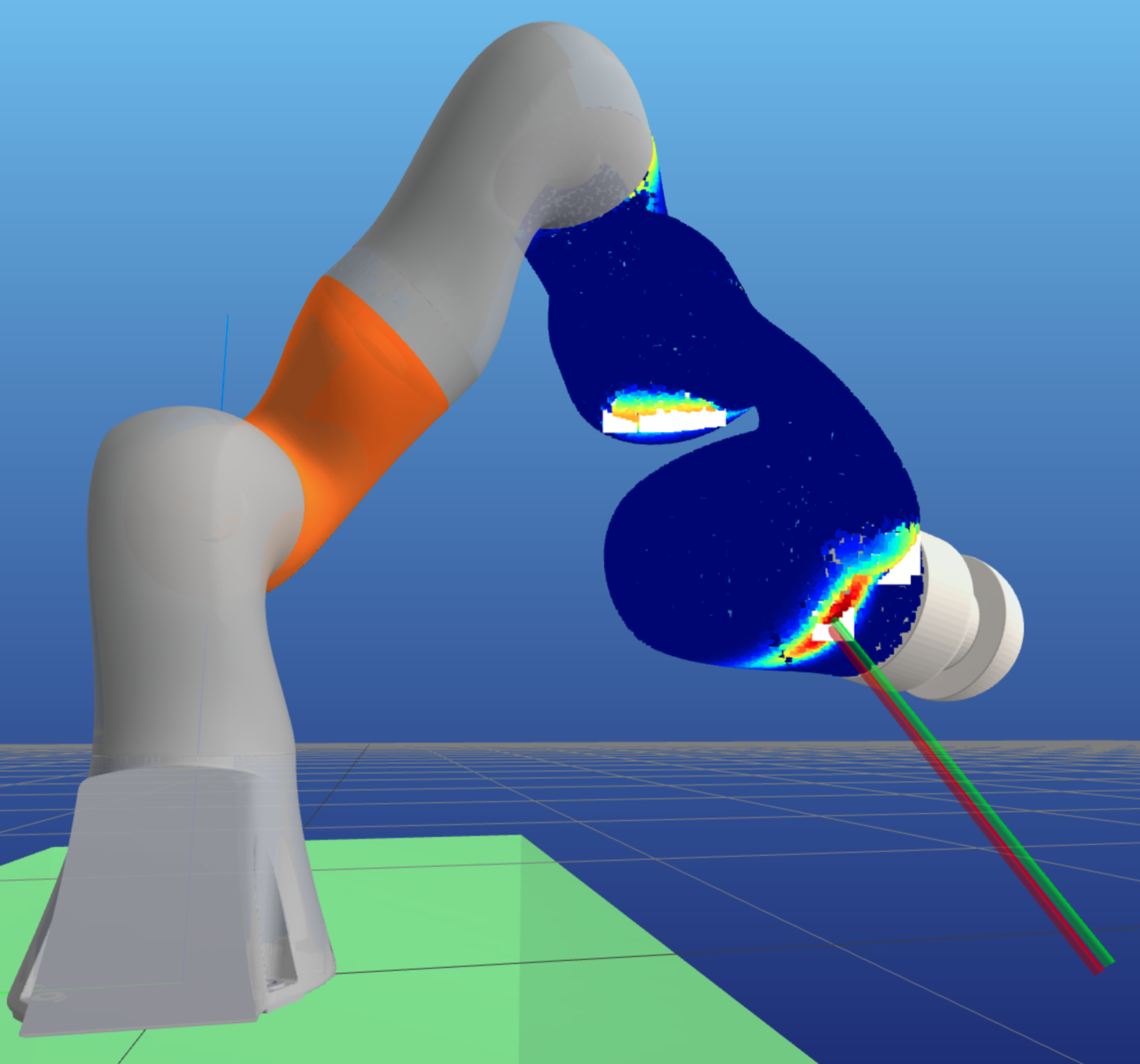
- The samples start uniformly distributed on \(\mathcal{S}\). Re-sampling is weighted by
- Unlike the Haddadin method, CPF always converge to a point on the robot.
Manuelli, L. and Tedrake, R., 2016, October. Localizing external contact using proprioceptive sensors: The contact particle filter. In 2016 IEEE/RSJ International Conference on Intelligent Robots and Systems (IROS) (pp. 5062-5069). IEEE
l(\bm{\tau_\text{ext}, p, q}) \coloneqq
\underset{\bm{v_f} \geq 0}{\text{min}} \; \| \bm{J}(\bm{q}, \bm{p})^{\intercal} \bm{v_f} - \bm{\tau}_\text{ext} \|^2
\underset{\bm{v_f} \geq 0 \; \bm{p} \in \mathcal{S}}{\text{min}} \; \| \bm{J}(\bm{q}, \bm{p})^{\intercal} \bm{v_f} - \bm{\tau}_\text{ext} \|^2
\exp{ -\frac{l(\bm{\tau_\text{ext}, p, q})}{\sigma^2}}
\(l = 0\)
\(l \) large
10000 samples / link
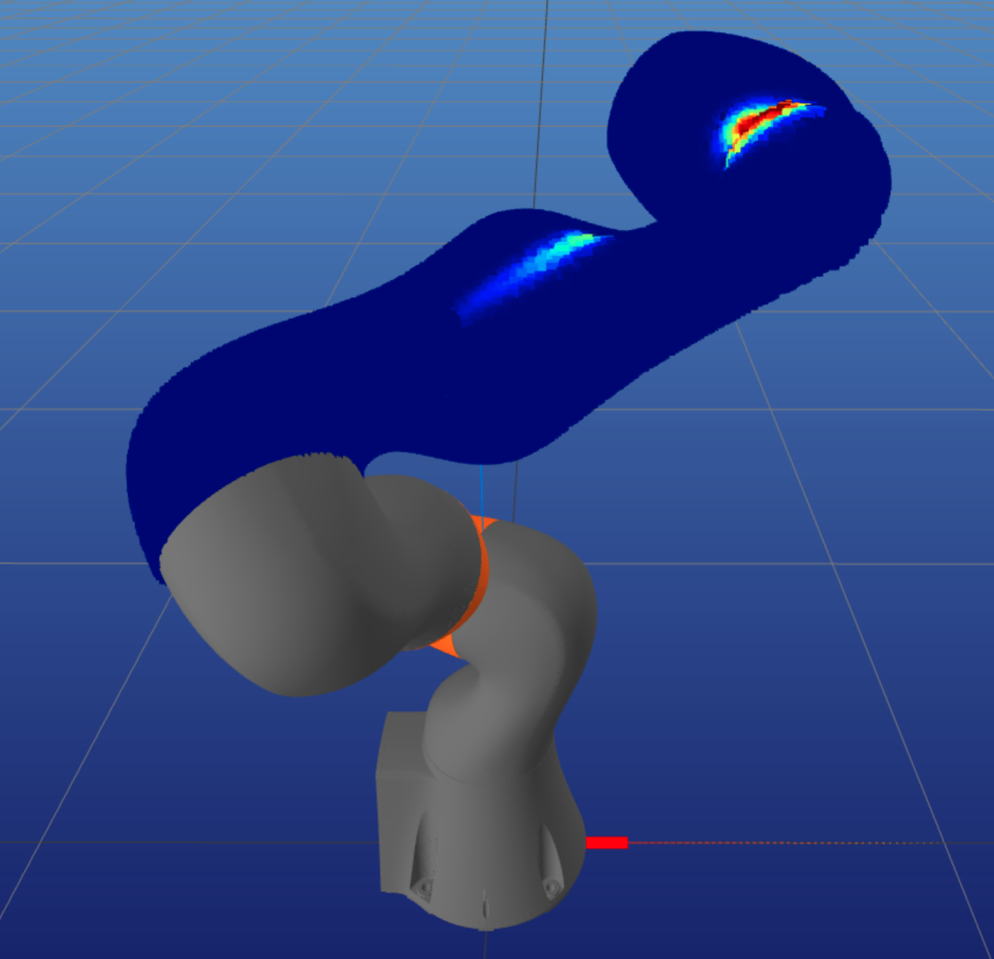
But there could be more than one \( \bm{p} \) where \( l(\bm{\tau_\text{ext}, p, q}) = 0 \)
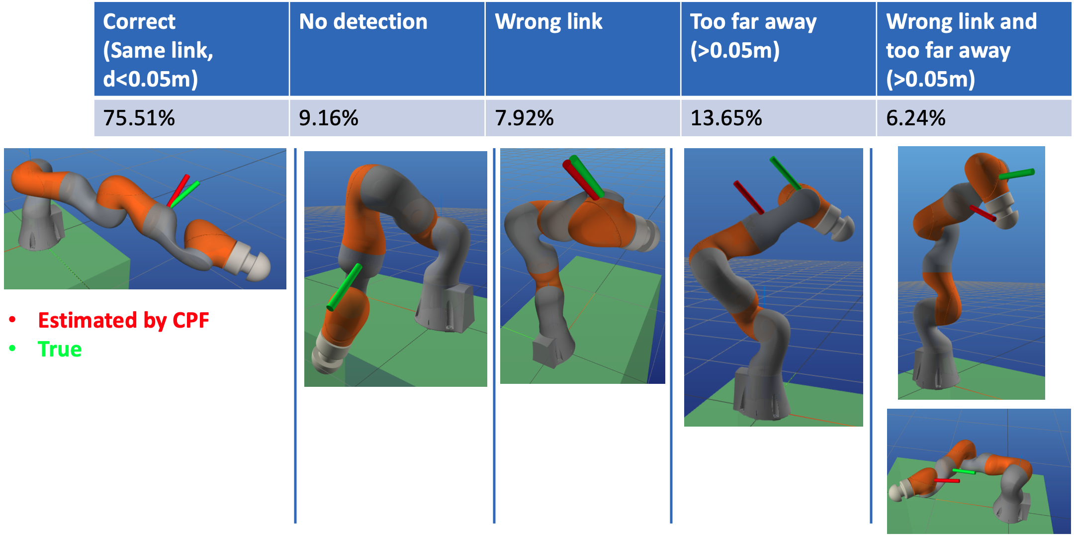
Some contacts can be explained equally well by multiple contact locations.
Out of 10000 randomly generated configuration and contacts, how often does contact particle filter fail to identify the true contact location?
25%
l(\bm{\tau_\text{ext}, p, q}) \coloneqq
\underset{\bm{v_f} \geq 0}{\text{min}} \; \| \bm{J}(\bm{q}, \bm{p})^{\intercal} \bm{v_f} - \bm{\tau}_\text{ext} \|^2
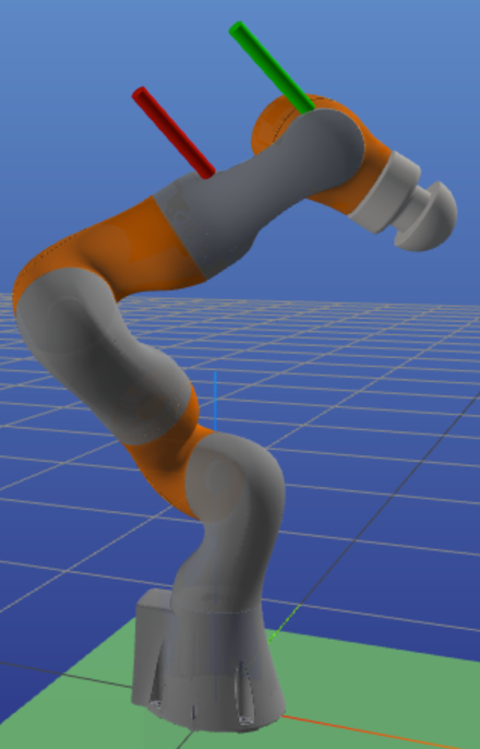
CPF failure modes
Multiple Local Minima of \(l\)
\(l = 0\)
\(l \) large
Where on \(\mathcal{S}\) is \( \| \bm{J}(\textcolor{blue}{\bm{q}}, \bm{p})^{\intercal} \bm{v_f} - \textcolor{blue}{\bm{\tau}_\text{ext}} \|^2 = 0\)?
- \(\mathcal{S}\) is a triangle mesh: \( \textcolor{green}{\bm{v}(\bm{p})} \) is a piecewise constant function of \(\bm{p}\).
- Even on a single piece, the objective function is nonlinear in the decision variables:
- And there are tens of thousands of pieces!
\underbrace{\bm{J}(\textcolor{blue}{\bm{q}}, \bm{p})}_{n_v \times n_q}\bm{v_f} =
\underbrace{\textcolor{green}{\bm{v}(\bm{p})^\intercal}}_{n_v \times 3}
\underbrace{
\begin{bmatrix}
-\hat{\bm{p}} & \textcolor{blue}{\bm{I}_3}
\end{bmatrix}
}_{3 \times 6}
\underbrace{\textcolor{blue}{\bm{J}_L(\bm{q})}}_{6 \times n_q}
\bm{v_f}
Constants
L
Alternative strategy
- Describing the set \( P_0 \coloneqq \{\bm{p} \in \mathcal{S} : l( \textcolor{blue}{\bm{\tau_\text{ext}}, \bm{q}}, \bm{p}) = 0\} \) is hard.
- Contact estimation from a single \(\bm{\tau}_\text{ext}\) can be ambiguous.
- But sampling from \( P_\epsilon \coloneqq \{\bm{p} \in \mathcal{S} : l( \textcolor{blue}{\bm{\tau_\text{ext}}, \bm{q}}, \bm{p}) \leq \epsilon\} \) is easier.
- New strategy:
- Find a set of samples: \( \overline{P}_{\epsilon} \subset P_{\epsilon} \) using rejection sampling.
- Run gradient descent on all \( \bm{p} \in \overline{P}_{\epsilon} \), creating a new set of converged samples: \( \overline{P}_{\epsilon}^* \)
- Ask the robot to collect more data to find the true contact from \( \overline{P}_{\epsilon}^* \) (TODO).
l( \textcolor{blue}{\bm{\tau_\text{ext}}, \bm{q}}, \bm{p}) \coloneqq
\underset{\bm{v_f} \geq 0}{\text{min}} \; \| \bm{J}(\bm{q}, \bm{p})^{\intercal} \bm{v_f} - \bm{\tau}_\text{ext} \|^2 \\

10000 samples / link
10000 samples / link
1000 samples / link
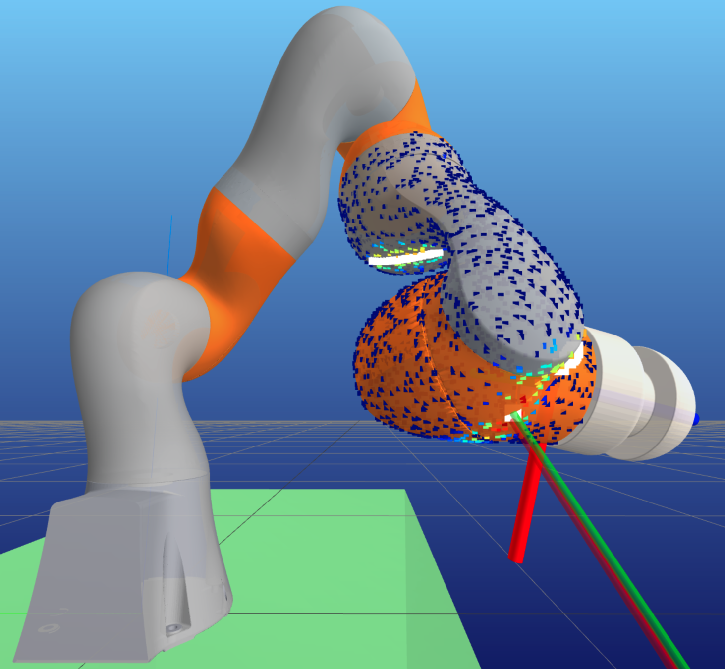
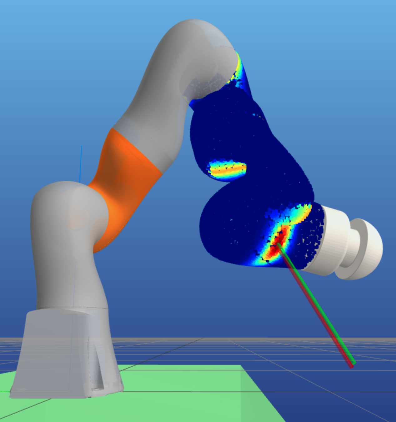
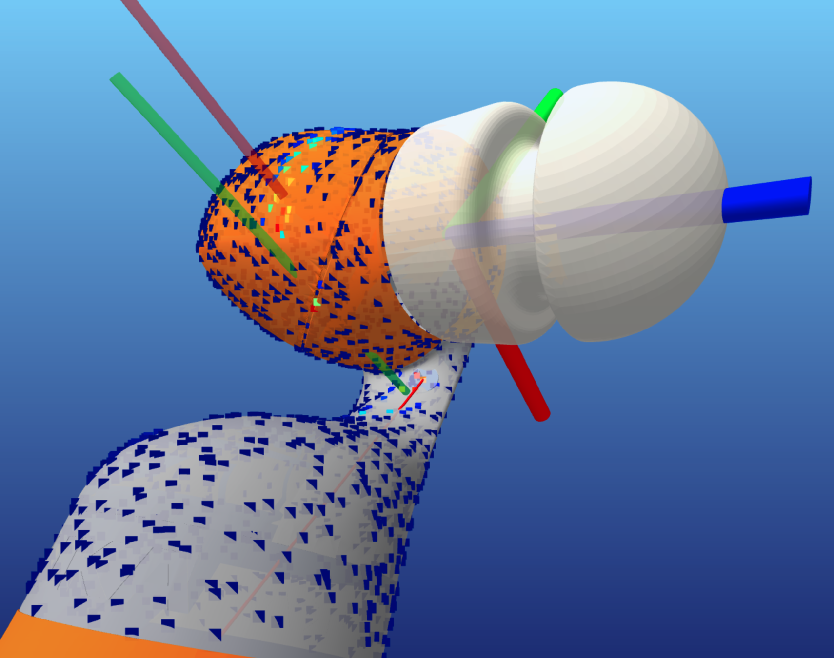
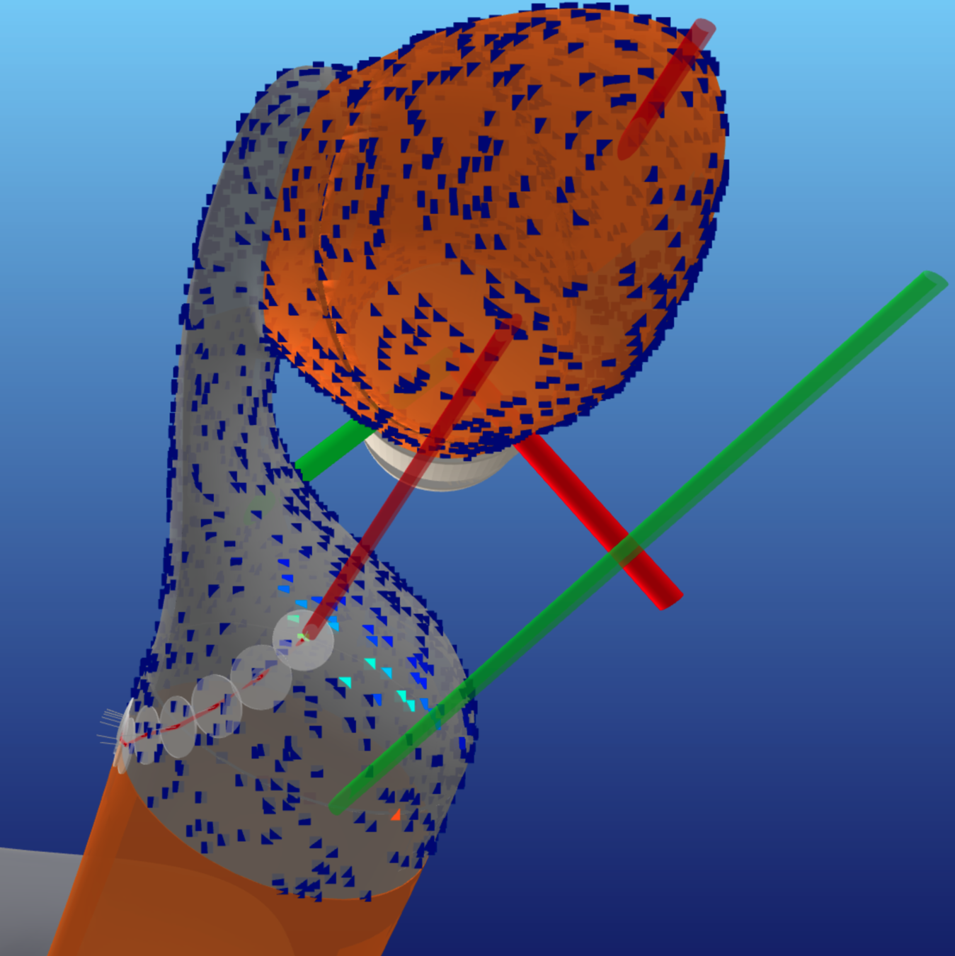
\( \overline{P}_\epsilon^* \) : white points.
Gradient descent
\( P_\epsilon \): points in white box
Gradient descent on \( \mathcal{S}\)
while \( \| \nabla_\bm{p} l \| \geq \epsilon \):
- project \( \nabla_\bm{p} l \) to the plane of the triangle of \( \bm{p} \).
- descend along the projected gradient to a new point \( \bm{p}^+ \) using line search.
- project \( \bm{p}^+ \) back to the mesh.
test idx: 1343
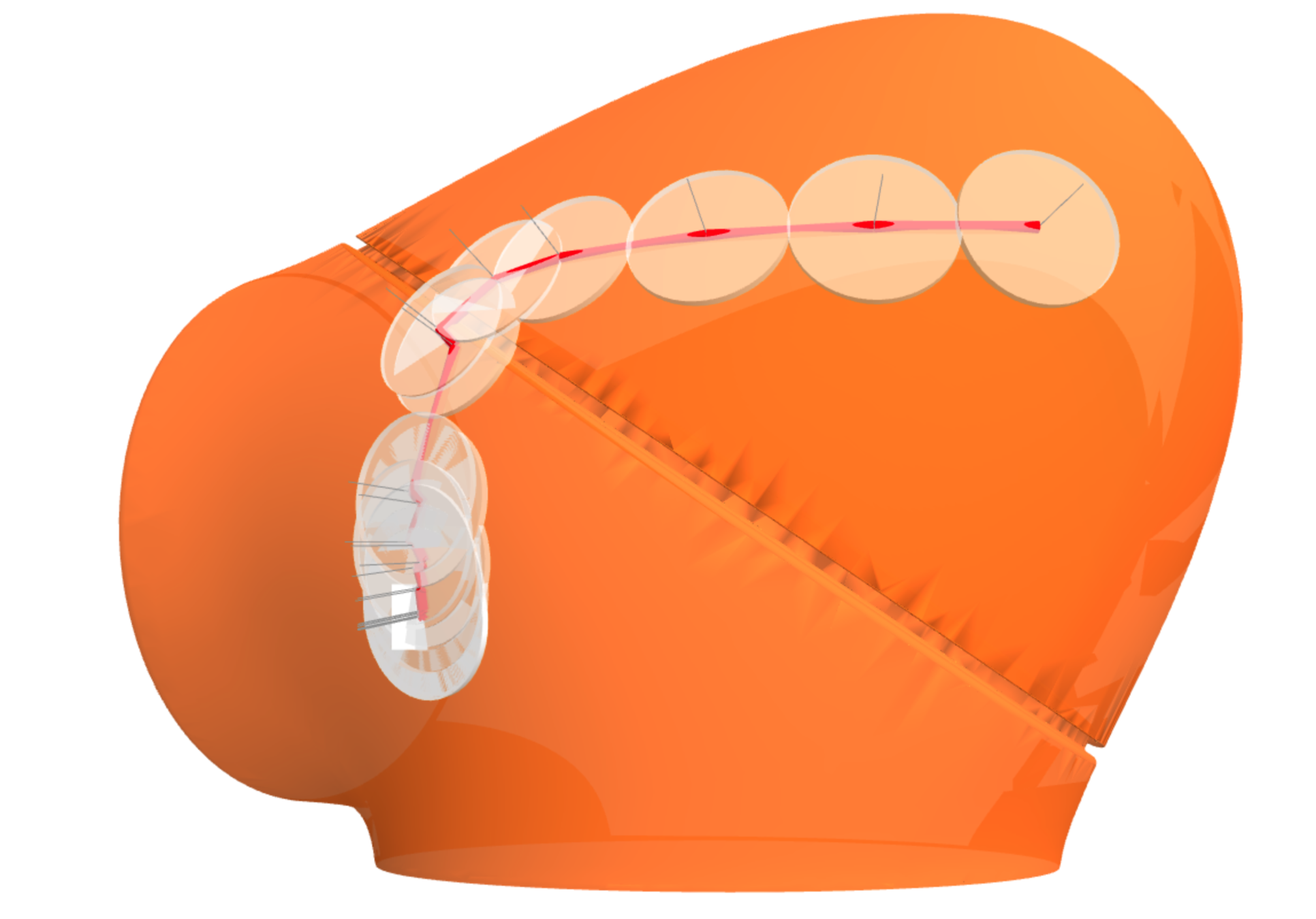
link 6
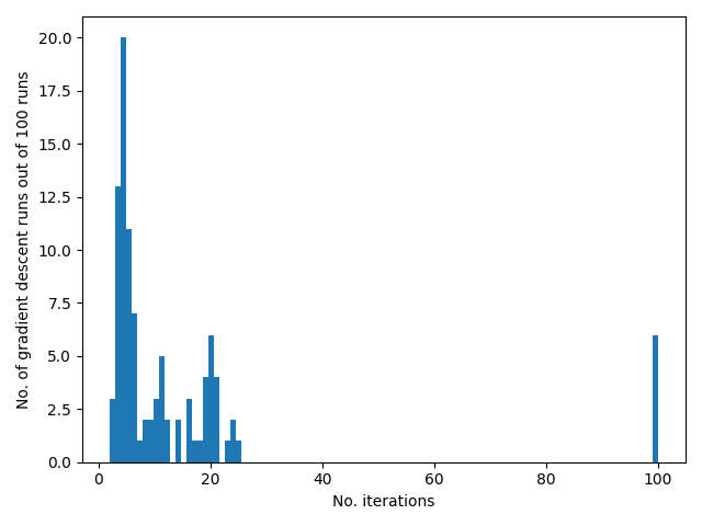
How fast do they converge?
(Show this in meshcat)
How well does this work?
| No. Tests | Gradient Descent successes* | Success% | GD w/ Rejection successes |
Success% | |
|---|---|---|---|---|---|
| CPF succeeds | 7551 | 7326 | 97% | ||
| CPF no detection | 916 | 874 | 95% | ||
| CPF too far away | 1365 | 1112 | 81% | 1255 | 92% |
- * Success means the true contact location is within 1cm of at least 1 of the samples gradient descent converges to.
- 50 gradient descents are run on each link, with number of iterations capped at 100.
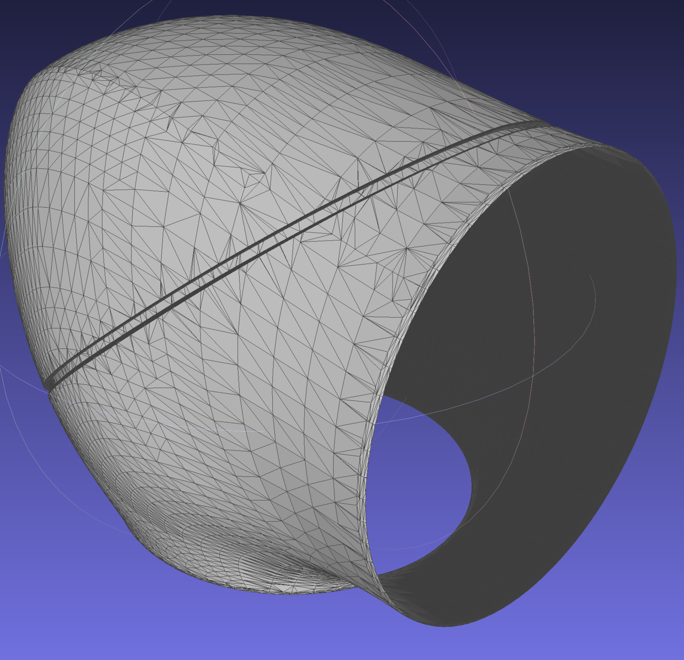
Failure modes
-
Many of the failures are due to anomalies in the mesh: "grooves (test 9701) and ledges".
-
Improve mesh quality.
-
-
Some are due to failures in proximity queries
-
Use signed distance field instead of bounding volume hierarchy?
-
Flipped normal
test id 4838
Proximity query returns a point "off-mesh".
test id 510
True contact on a "ledge", not covered by samples. Therefore the local minimum doesn't exist on the robot surface.
test id 868
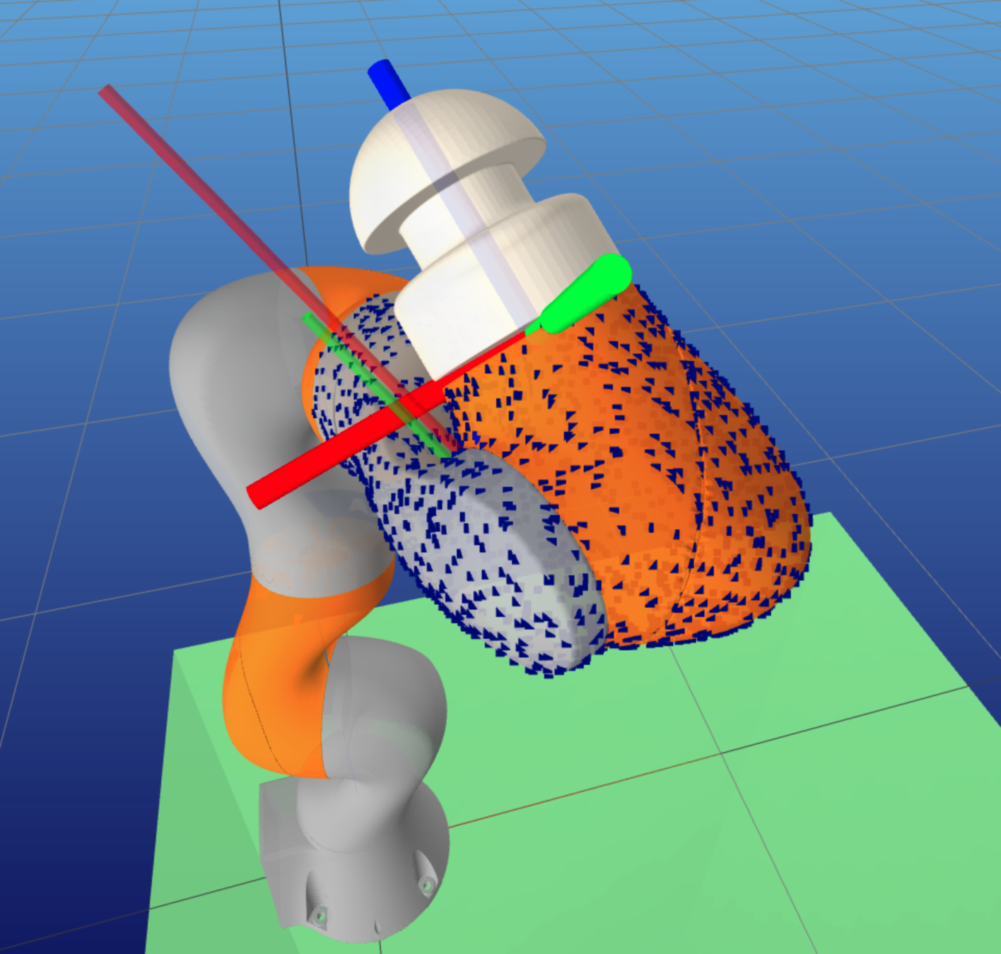
What does \( \overline{P}_\epsilon \) look like?
- White squares are members of \( \overline{P}_\epsilon \).
- Generated from 100 samples (50 / link).
- Number of converged samples: 23.
Alternative strategy
- Describing the set \( P_0 \coloneqq \{\bm{p} \in \mathcal{S} : l( \textcolor{blue}{\bm{\tau_\text{ext}}, \bm{q}}, \bm{p}) = 0\} \) is hard.
- But sampling members of \(P^* \coloneqq \{\bm{p} \in \mathcal{S} : \nabla_\bm{p} l ( \textcolor{blue}{\bm{\tau_\text{ext}}, \bm{q}}, \bm{p}) = 0\}\) is easier.
- \( P_0 \subset P^{*} \) (?)
- Members of \( P^* \) can be found by gradient descent, starting from any \(\bm{p} \in \mathcal{S}\). The gradient is given by
- Running gradient descent from many initial positions gives samples from \(P^*\): \( \overline{P}^* \subset P^* \).
- We can form a new set \( \overline{P}^*_\epsilon \coloneqq \{ \bm{p} \in \overline{P}^*: l( \textcolor{blue}{\bm{\tau_\text{ext}}, \bm{q}}, \bm{p}) \leq \epsilon \}\).
- To find the true contact location from \( \overline{P}^*_\epsilon\), we can compute a robot motion to collect more measurements (ongoing work).
l( \textcolor{blue}{\bm{\tau_\text{ext}}, \bm{q}}, \bm{p}) \coloneqq
\underset{\bm{v_f} \geq 0}{\text{min}} \; \| \bm{J}(\bm{q}, \bm{p})^{\intercal} \bm{v_f} - \bm{\tau}_\text{ext} \|^2 \\
= \underset{\bm{v_f} \geq 0}{\text{min}} \; \left(\bm{v_f}^\intercal \underbrace{\bm{J}\bm{J}^\intercal}_{\bm{Q}} \bm{v_f} - 2 \left(\underbrace{\bm{J} \bm{\tau}_\text{ext}}_{-\bm{b}}\right)^\intercal \bm{v_f} + \bm{\tau}_\text{ext}^\intercal \bm{\tau}_\text{ext} \right)
\nabla_\bm{p} l =
\textcolor{red}{\frac{\partial l}{\partial Q}} \frac{\partial Q}{\partial \bm{p}} +
\textcolor{red}{\frac{\partial l}{\partial b}} \frac{\partial b}{\partial \bm{p}}
From KKT conditions.
From AutoDiff.
Contact Detection from Joint Torque Measurements
By Pang


