iRS-RRT
Pang, Terry, Lu
the Story
Q: how do we solve long horizon, planning through contact problems?
- Deep learning is impressive. But learned policies do not generalize to different tasks.
- So far, methods based on physics models suffer from the huge number of contact modes.
- Contact modes manifest as complementarity constraints in trajectory optimization. They can be mitigated with numerical tricks, but in general are sensitive to initial guesses and cost tuning.
- For simpler systems, contact modes can be enumerated. Discrete mode planning and continuous state planning can be interleaved in a sampling-based planning algorithm. But this would not scale to tasks such as 3D dexterous manipulation.
- In this work, we propose to replace the reasoning about contact modes with their statistical summary into locally linear systems, which we call bundled dynamics.
- We show the power of bundled dynamics with some simple modifications to the standard kino-dynamic RRT.
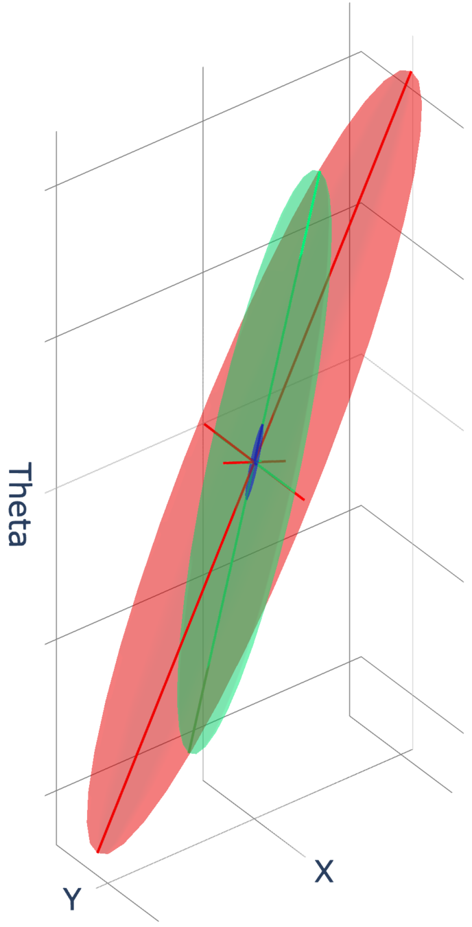
Reachable Set on Bundled Dynamics
Let's motivate the Gaussian from a different angle.
\begin{aligned}
x_{t+1} & = \hat{\mathbf{A}}x_t + \hat{\mathbf{B}} u_t + (\hat{f}(x_t,u_t) - \hat{\mathbf{A}}x_t - \hat{\mathbf{B}}u_t) \\
& = \hat{\mathbf{A}}x_t + \hat{\mathbf{B}} u_t + \hat{c}_t
\end{aligned}
Recall the linearization of bundled dynamics around a nominal point.
\begin{aligned}
\hat{\mathbf{B}} = \mathbb{E}\bigg[\frac{\partial f}{\partial u}(\bar{x}_t, \bar{u}_t + w)\bigg]
\end{aligned}
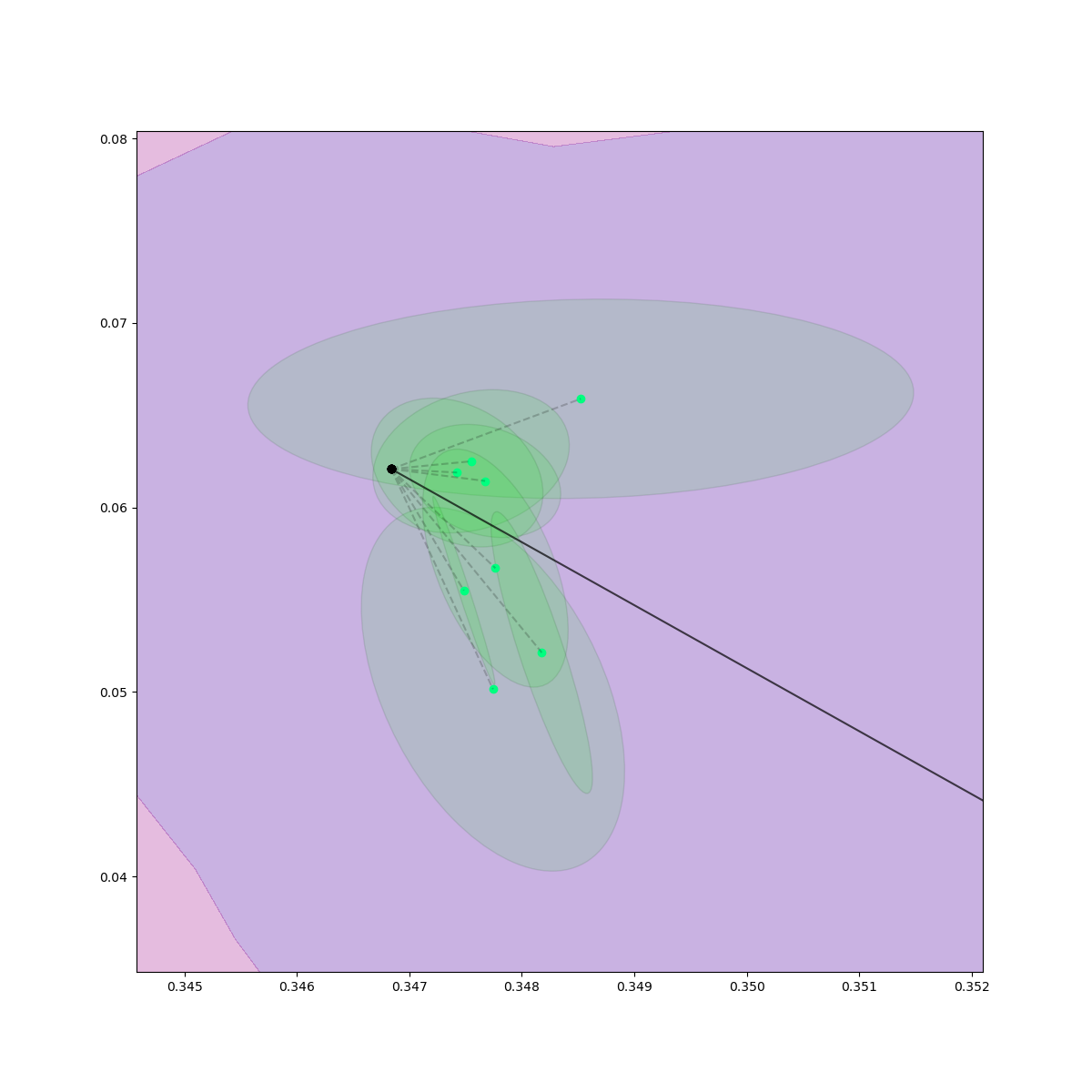
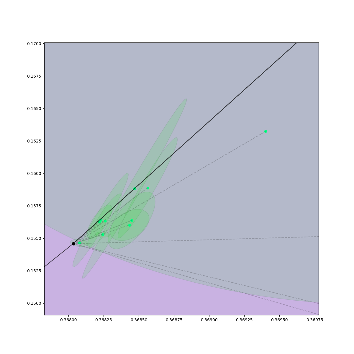
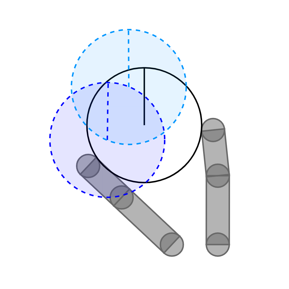
Fixing the state, we reason about the states that are reachable under the bundled dynamics under some input.
(Image of the input norm-ball under bundle dynamics, assume \bar{u}_t is zero.)
\begin{aligned}
\mathcal{S} & = \{\hat{x}_{t+1} | \hat{x}_{t+1} = \hat{\mathbf{B}} u_t + \hat{f}(\bar{x}_t, 0), \|u_t\| \leq \varepsilon\} \\
& = \{\hat{x}_{t+1} | (\hat{x}_{t+1} - \hat{f}(\bar{x}_t, 0))^\intercal \big[\hat{\mathbf{B}}\hat{\mathbf{B}}^\intercal\big]^{-1} (\hat{x}_{t+1} - \hat{f}(\bar{x}_t, 0)) \leq \varepsilon^2\}
\end{aligned}
The latter expression becomes the eps-norm ball under Mahalanabis metric.
Distance Metric Based on Local Actuation Matrix
\begin{aligned}
\|x\|_{\Sigma^{-1}}^2 & = x^\intercal \big[\mathbf{B}\mathbf{B}^\intercal\big]^{-1} x
\end{aligned}
Consider the distance metric:
This naturally gives us distance from one point in state-space another as informed by the actuation
(i.e. 1-step controllability) matrix.
NOTE: This is NOT a symmetric metric for nonlinear dynamical systems. (even better!)
Rows of the B matrix.
\begin{aligned}
A
\end{aligned}
\begin{aligned}
B
\end{aligned}
A is harder to reach (has higher distance) than B even if they are the same in Euclidean space.
Handling Singular Cases
\begin{aligned}
\text{rank}\big[\mathbf{B}\mathbf{B}^\intercal\big] < n
\end{aligned}
What is B is singular, such that
The point that lies along the null-space is not reachable under the current linearization. So distance is infinity!
Numerically, we can choose to "cap" infinity at some finite value by introducing regularization.
Rows of the B matrix.
\begin{aligned}
A
\end{aligned}
There is loss of 1-step controllability and A is unreachable. Infinite distance.
\begin{aligned}
x^\intercal \big[\mathbf{B}\mathbf{B}^\intercal + \lambda \mathbf{I}\big]^{-1} x = \min \big\{x^\intercal \big[\mathbf{B}\mathbf{B}]^{-1} x, \lambda^{-1}\big\}
\end{aligned}
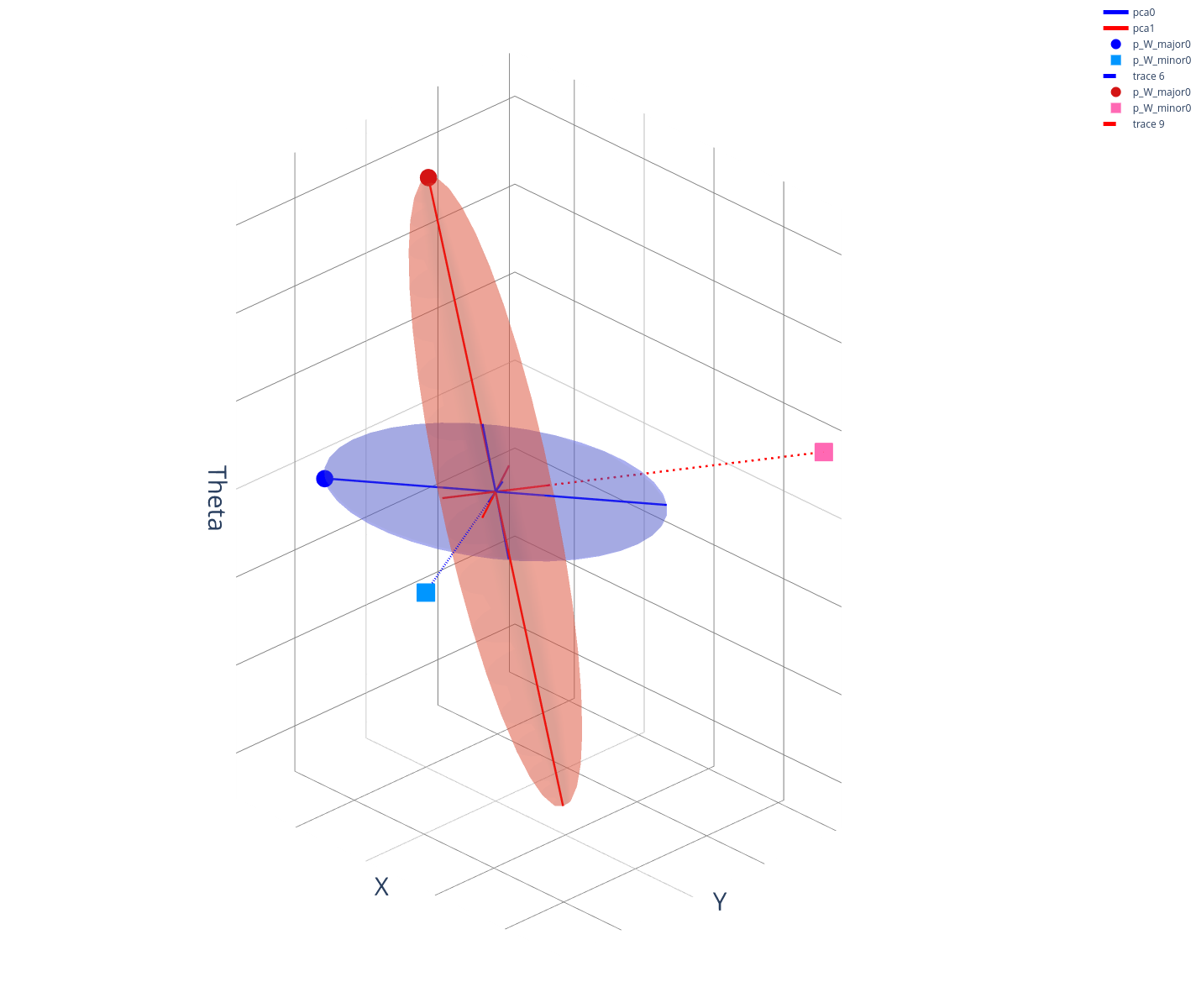
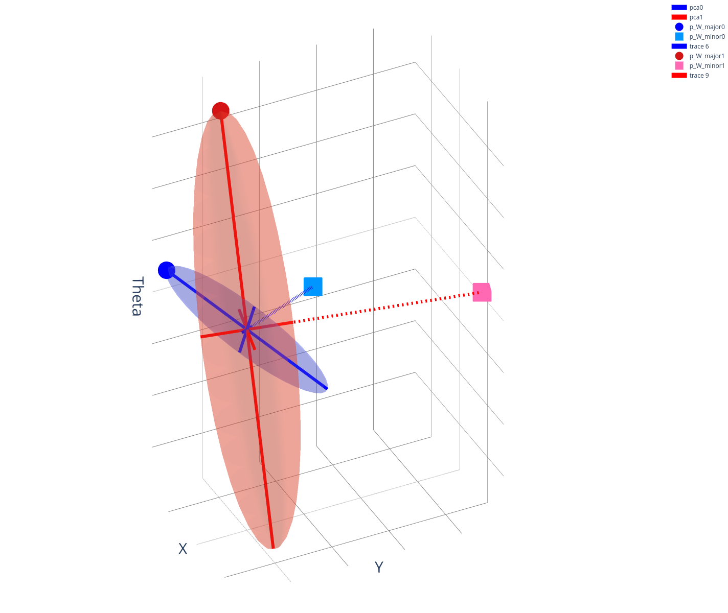
Connection to Gaussian Covariance Estimation
We can obtain the covariance matrix of the ellipse directly using gradient information, but we can also consider the zero-order version that solves the least-squares problem:
\begin{aligned}
\hat{\mathbf{B}} & = \text{argmin} \sum_i \|\hat{f}(\bar{x}, u_t^i) - \mathbf{B} u_t^i\|
\end{aligned}
Under the least-squares solution, one can show a connection between directly doing covariance estimation on samples.
Consider putting the above into data matrix form
\begin{aligned}
\hat{\mathbf{B}} & = \text{argmin} \|\mathbf{F} - \mathbf{B}\mathbf{X}\|^2_2 \\
& = \mathbf{V}\Sigma^{-1}\mathbf{U}^\intercal \mathbf{F}
\end{aligned}
where X is data matrix of u that is sampled from zero-mean Gaussian and diag. covariance of sigma.
\begin{aligned}
\mathbb{E}[\hat{\mathbf{B}}\hat{\mathbf{B}}^\intercal] & = \frac{1}{\sigma^2 (N-1)} \mathbb{E}[\mathbf{F}\mathbf{F}^\intercal]
\end{aligned}
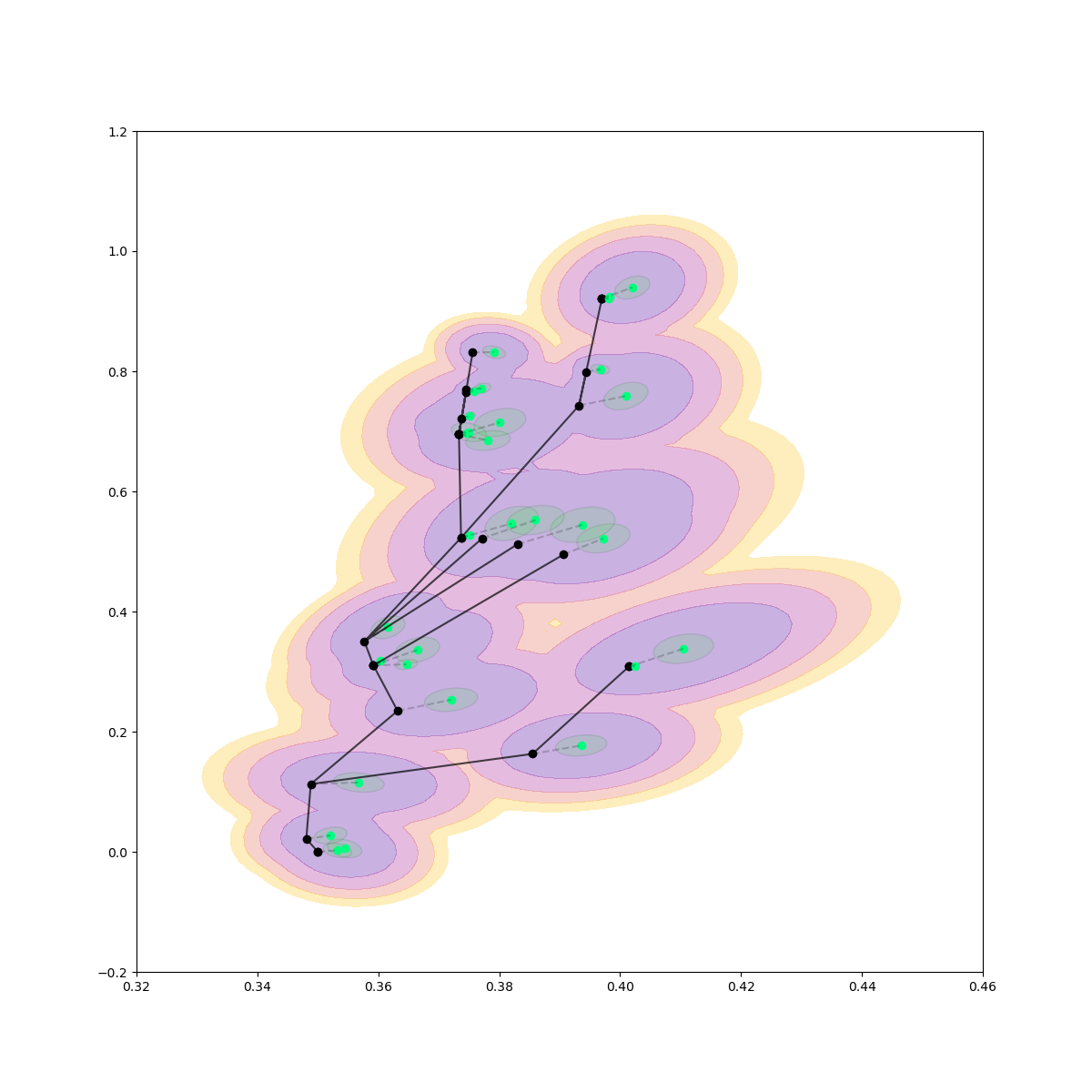
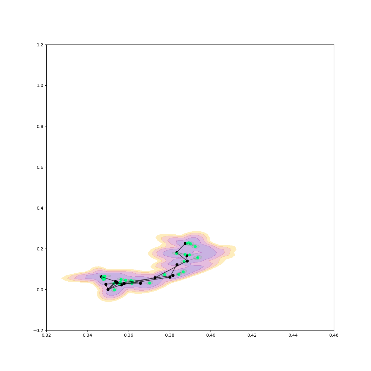
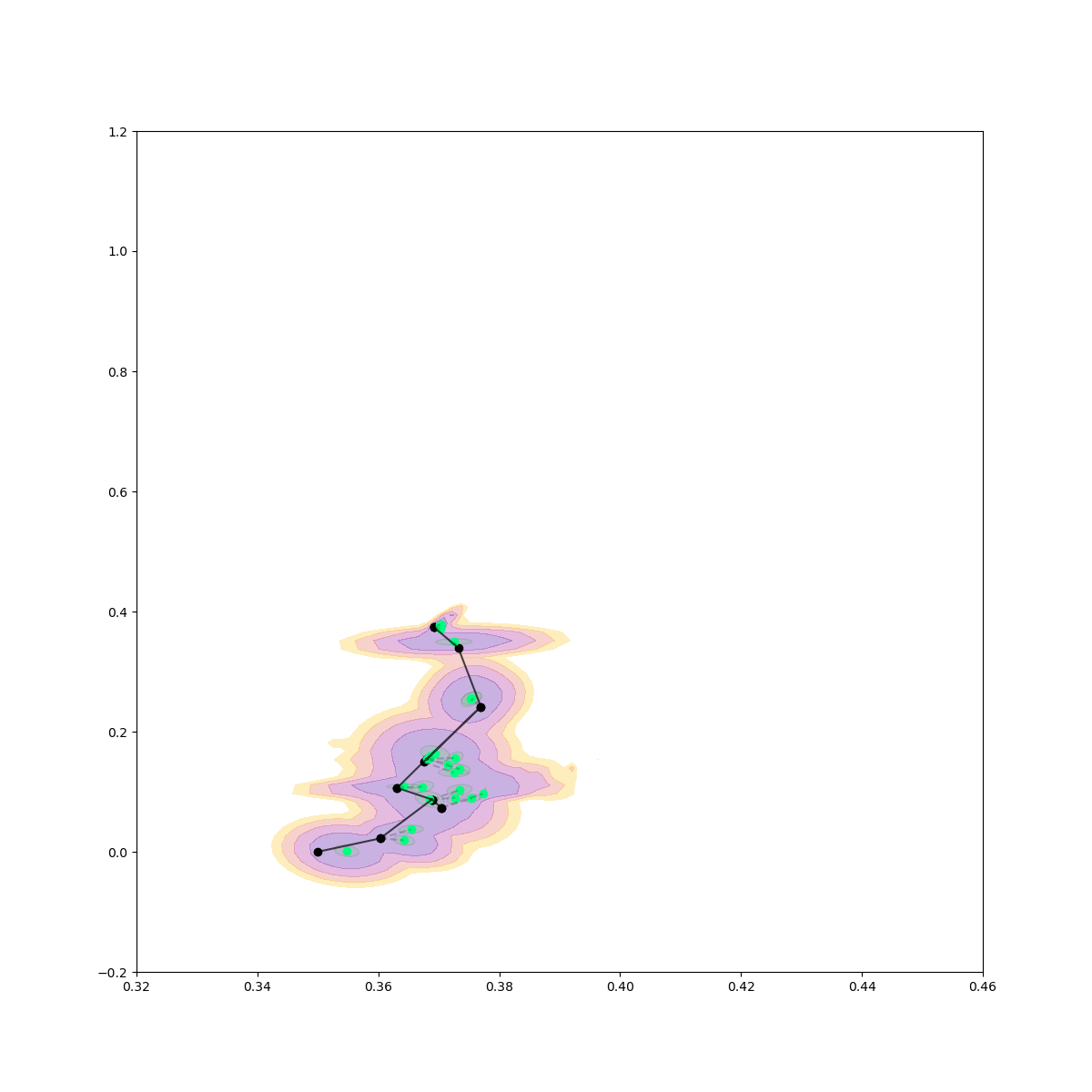
How bundled dynamics helps in kino-dynamic RRT
- RG-RRT uses local reachability information to guide subgoal sampling towards more reachable part of the smooth space.
- Bundled dynamics provides good reachability info for systems with contact.
- By helping with 1 or T-step trajectory optimization in extension (the same story as iRS-MPC).
- There's a trade-off between the number of nodes and the planning horizon T.
Rejection Sampling / Contact Sampling
Rejection Sampling + Contact Sampling
No Contact Sampling
No Rejection Sampling
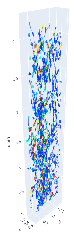
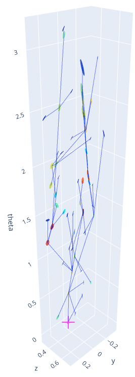
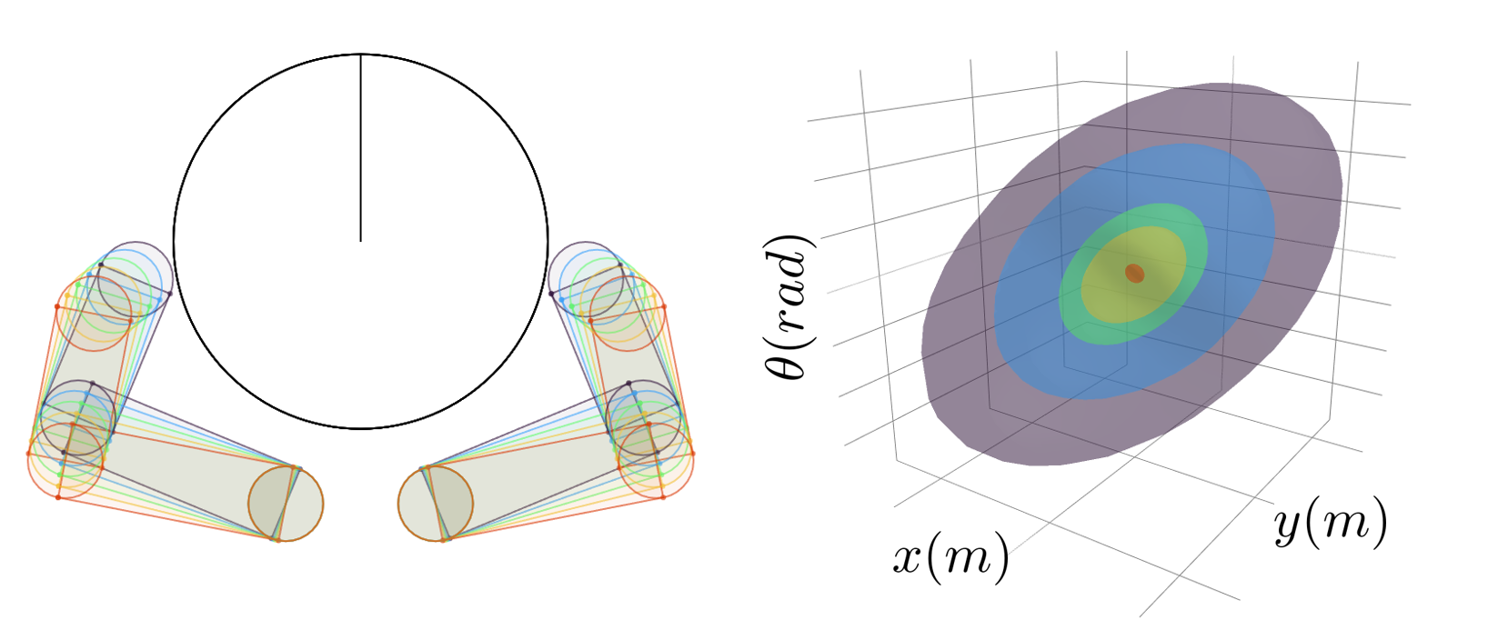
Results
- Planar pushing
- Planar hand
- Allegro hand
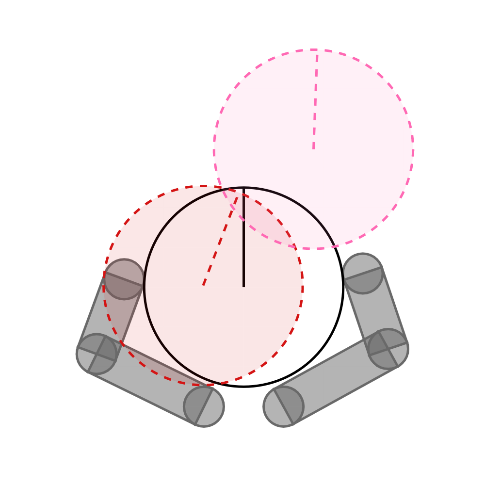
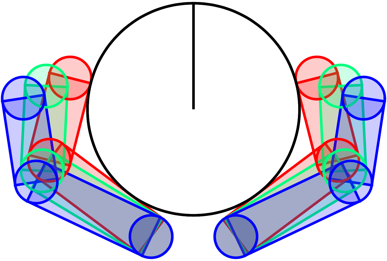
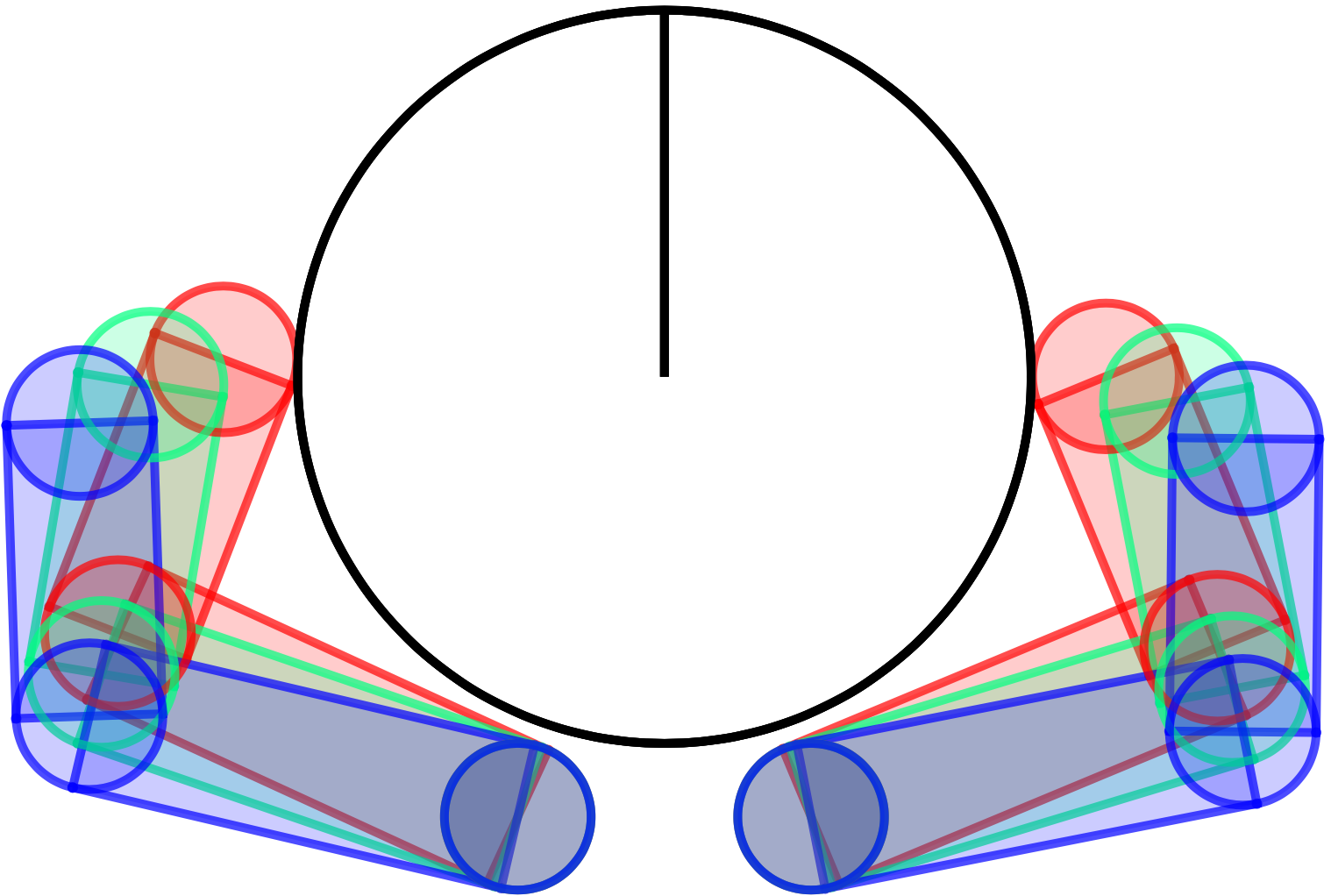
Planar Hand
1-step extension
20-step extension
(b1)
(b2)
(b1)
(b2)
(c1)
(c2)
(c1)
(c2)
(a)
(b)
(c)
x - \hat{x}
y - \hat{y}
\theta - \hat{\theta}
x
y
x
y
(d)
(a)
(b)
(c)
x - \hat{x}
y - \hat{y}
\theta - \hat{\theta}
x
y
x
y

b_1
b_2
c_1
c_2
b_1
b_2
c_1
c_2
(a)
(b)
(c)
x - \hat{x}
y - \hat{y}
\theta - \hat{\theta}
x
y
b_1
b_2
c_1
c_2
x - \hat{x}
b_1
b_2
c_1
c_2
x
y
(d)
(a)
(b)
(c)
y - \bar{y}
\theta - \bar{\theta}
x
y
b_1
b_2
c_1
c_2
x - \bar{x}
b_1
b_2
c_1
c_2
x
y
(d)
x - \bar{x}
y - \bar{y}
\theta - \bar{\theta}
planning_through_contact_Feb_2022
By Pang


